
Estimating Effective Leaf Area Index of Winter Wheat Based on UAV Point Cloud Data
by
 , and
, and
Jie Yang
1,2,
Minfeng Xing
1,2,*,
Qiyun Tan
3,
Jiali Shang
4,
Yang Song
5,
Xiliang Ni
6,
Jinfei Wang
7 and
Min Xu
8 1
School of Resources and Environment, University of Electronic Science and Technology of China, Chengdu 611731, China
2
Yangtze Delta Region Institute (Huzhou), University of Electronic Science and Technology of China, Huzhou 313001, China
3
Beijing Yuhang Intelligent Technology Co., Ltd., Beijing 100193, China
4
Agriculture and Agri-Food Canada, Ottawa, ON K1A0C6, Canada
5
Intelligent Agriculture Research Institute, Zoomlion Smart Agriculture, Changsha 410013, China
6
Ministry of Education Key Laboratory of Ecology and Resource Use of the Mongolian Plateau & Inner Mongolia Key Laboratory of Grassland Ecology, School of Ecology and Environment, Inner Mongolia University, Hohhot 010021, China
7
Department of Geography and Environment, University of Western Ontario, London, ON N6A5C2, Canada
8
The State Key Laboratory of Remote Sensing Science, Aerospace Information Research Institute, Chinese Academy of Sciences, Beijing 100101, China
*
Author to whom correspondence should be addressed.
Drones 2023, 7(5), 299; https://doi.org/10.3390/drones7050299
Submission received: 15 March 2023
/
Revised: 16 April 2023
/
Accepted: 29 April 2023
/
Published: 3 May 2023
Abstract
:Leaf area index (LAI) is a widely used plant biophysical parameter required for modelling plant photosynthesis and crop yield estimation. UAV remote sensing plays an increasingly important role in providing the data source needed for LAI extraction. This study proposed a UAV-derived 3-D point cloud-based method to automatically calculate crop-effective LAI (LAIe). In this method, the 3-D winter wheat point cloud data filtered out of bare ground points was projected onto a hemisphere, and then the gap fraction was calculated through the hemispherical image obtained by projecting the sphere onto a plane. A single-angle inversion method and a multi-angle inversion method were used, respectively, to calculate the LAIe through the gap fraction. The results show a good linear correlation between the calculated LAIe and the field LAIe measured by the digital hemispherical photography method. In particular, the multi-angle inversion method of stereographic projection achieved the highest accuracy, with an R2 of 0.63. The method presented in this paper performs well in LAIe estimation of the main leaf development stages of the winter wheat growth cycle. It offers an effective means for mapping crop LAIe without the need for reference data, which saves time and cost.
1. Introduction
Leaf area index (LAI) is an important parameter in modelling vegetation photosynthesis and evapotranspiration, and plays an essential role in material exchange and energy flow between soil, vegetation, and atmosphere [1]. LAI is defined as the total of one-sided leaf area per unit of ground surface area [2]. LAI is of great significance for crop growth monitoring and accurate yield forecast.
LAI can be measured directly and indirectly. The direct measurement method involves collecting plant leaves destructively and directly measuring their area. This method has high accuracy, but it is labor-intensive and time-consuming. Therefore, it is not operationally feasible to apply over large areas or multiple times throughout the growing season [3]. Indirect LAI measurements can be achieved by correlating total leaf area with the probability of light penetration through a canopy, and the LAI can be estimated indirectly using optical instruments. It has the advantage of being non-destructive and efficient, and it has been widely used [3,4]. Indirect measurements mainly include inclined-point quadrats and optical methods. Warren, Wilson, and Reeve developed the method of inclined-point quadrats for LAI based on counting the number of leaves contacted by a sharp metal probe passing through a canopy at various angles [5]. A slender probe was inserted into the canopy at a fixed angle of inclination, and the leaf area index was calculated by recording the average number of probes in contact with the leaf in the unit cm depth layer [5,6]. The inclined-point quadrats method requires a large number of probes, and it is not easy to count accurately the number of contacts between the probes and leaves, which makes it difficult to implement for large canopies. The diameter of the probe is a major factor causing errors. Optical methods use mathematical equations and radiative transfer theory to estimate the LAI from more easily and quickly measurable variables, such as gap fraction or gap size distribution, which are based on measurements of light transmission through canopies [7,8]. Among these methods, Beer’s law-based optical methods have become the mainstream approach for LAI measurement [9]. They have been implemented with multiple commercial optical instruments, including the LAI-2000 Plant Canopy Analyzer (LI-COR, Lincoln, NE, USA), AccuPAR (Decagon Devices, Inc., Pullman, WA, USA) and Tracing Radiation and Architecture of Canopies (TRAC, 3rd Wave, Nepean, ON, Canada). In addition, the technology of Digital Hemispherical Photographs (DHPs) has been developed [7,8,9,10,11]. Thus, these methods are widely used for ground measurement and remote sensing validation.
Ground LAI measurements can usually be collected over a small area, and it is not feasible to provide the data volume required for national, regional, and global applications. Remote sensing provides an alternative data source for LAI retrieval and has been increasingly used in agricultural applications [12,13]. Remotely sensed LAI can be used for crop monitoring and yield estimation at different scales, providing support for producer management decisions. Zhang et al. used MODIS LAI of the growing season to estimate country-level crop production in European countries and regional-level crop production in United States [14]. Huang et al. assimilated LAI obtained from Landsat TM and MODIS data into the WOFOST crop growth model to predict regional-scale winter wheat yield [15]. Song et al. applied the modified SAFY-height model on crop height and LAIe maps derived from a UAV-based SfM point cloud to predict winter wheat yield in sub-fields [16].
There are two modelling approaches to retrieve LAI from remote sensing data, statistical models and physical models. The statistical model approach calculates the vegetation index (VI) from the remote sensing image data and establishes a single-factor or multi-factor model of VI and LAI. The model is then used to map the LAI of the area of interests [17]. Statistical models for LAI retrieval can be built through either parametric or non-parametric regression. Parametric regression models, including linear and exponential models, are simple and easy to understand, but the existing spectral information is not fully utilized, and the inversion accuracy largely depends on the spectral bands used. In contrast, non-parametric regression models, such as the partial least squares regression (PLS), back propagation (BP) network, support vector machine (SVM), and random forest (RF), make full use of the spectral information and have high nonlinear adaptive ability. However, one of their main disadvantages is their instability when applied to datasets that deviate from the training dataset. Hybrid methods also exist which combine both. All in all, the method based on statistical modelling is simple, easy to operate, and has strong operability. It is one of the commonly used methods in the remote sensing inversion of parameters such as LAI. However, the model mechanism is not clear and has inherent regional influence. The VI value includes not only information about LAI, but also information about vegetation structure, vegetation coverage by the target crop, and other parameters, such as biomass, chlorophyll concentration, and photosynthetic effective absorption radiation (FAPAR). Thus, these methods are suitable for a small range of specific types of vegetation [18,19,20,21,22]. Methods based on physical models mainly consider the non-Lambertian characteristics and bidirectional reflection characteristics of vegetation canopy reflection, and inverts vegetation canopy parameters by constructing models of surface reflectance and biophysical parameters such as LAI, including radiative transfer (RT) models, geometric optical (GO) models, RT/GO hybrid models, and Monte Carlo models. Although the physical models fully consider many influencing factors such as vegetation leaf structure characteristics, soil background, and topography, which can truly reflect the vegetation canopy and provide good stability and adaptability, their inversion processes are complex and require a large number of input parameters, making them difficult to utilize, which limits their operational application [18,19,20,21,22,23].
In recent years, with continuous improvement of the stability, safety, and controllability of Unmanned Aerial Vehicles (UAVs), UAV-based remote sensing for crop monitoring has progressed rapidly [24]. UAVs provide a cost-effective platform for various remote sensing acquisition of data including RGB imagery, multispectral, hyperspectral, LiDAR, microwave, and thermal data at very high spatial resolutions and with flexible acquisition windows [25]. Multi-source UAV data have been used to widely to retrieve crop biophysical parameters. Li et al. used color index and texture features extracted from UAV digital images to establish statistical models to estimate rice LAI [26]. Liu et al. used multi-source remote-sensing data, including RGB images, multispectral images, and thermal infrared images, collected from a UAV crop high-throughput phenotyping platform, to develop a multimodal data-processing DL framework based on DNN architecture to estimate corn LAI [27]. A study by Duan et al. used a physical-based approach to invert the PROSAIL model to estimate the LAI of corn, potato, and sunflower from UAV hyperspectral data [28]. Contrary to optical remote sensing, light range and detection (LiDAR) is an active remote sensing technology that has been used to invert forest gap fraction and LAI [29]. Point cloud data (PCD) generated with LiDAR include the three-dimensional coordinates, color, reflection intensity, echo times, and other information of the scanned target. PCD can also be generated from RGB images by structure from motion (SfM) technology [30,31]. LAI can be estimated through statistical models between plant geometric and structural parameters obtained from PCD and field-measured LAI. Jaume Arno’ et al. used a tractor-mounted LiDAR system to measure the height, the cross-sectional area, the canopy volume, and the tree area index of vines and performed a linear regression analysis of these parameters with the measured LAI to estimate LAI [32]. L. Comba et al. used a 3-D point cloud from UAV imagery to estimate LAI using a multivariate linear regression model on a subset of 15 crop canopy descriptors of vineyards, which included the canopy thickness, height, and leaf density distribution along the wall [33]. The above method requires additional field-measured LAI values to establish an empirical relationship, and the parameterization of specific objects and locations may not be suitable for other scenarios [34]. LAI is mainly estimated from PCD by means of correlation with gap fractions, mainly including two-dimensional and three-dimensional methods. In the three-dimensional method, the point cloud is voxelized and the distribution of empty and non-empty voxels is studied from a spatial perspective [35]. Although this method can take advantage of the three-dimensional advantages of PCD, it needs to directly operate the PCD with a huge amount of data, and requires more calculation [36]. The two-dimensional method converts the point cloud into black and white images (black or white pixels represent the canopy or background, respectively) to study the proportion of black and white pixels, which is easier to apply to practical work. There are many studies on gap assessment and LAI estimation of forest and individual tree canopies using the two-dimensional method based on PCD. Hancock et al. used the ray tracing method to convert the PCD of forest vegetation obtained by a ground-based laser radar scanner into a hemispherical black-and-white image to assess forest gap fraction [37]. Zheng et al. projected the TLS PCD onto a two-dimensional plane using spherical projection and two geometric projection methods to retrieve the LAIe of the forest stand [36]. However, there are differences between different platforms such as TLS and ALS in data scanning mode, point density, coverage, etc. Therefore, many quantitative retrieval methods of forest vegetation LAI cannot be generalized. To the best of our knowledge, there are few studies on the LAIe of winter wheat crop planting areas using the above two-dimensional method.
The cost of acquiring PCD from LiDAR is very high, and the subsequent data processing is complex and time consuming. As an alternative, the low-cost consumer-grade UAV system composed of RGB digital cameras and light UAVs has widespread use. The RGB images obtained by UAVs equipped with digital cameras can produce cost-effective 3-D PCD through SfM technology, which represents a low-cost remote sensing alternative to airborne and terrestrial LiDAR. In addition, this method has an unrivalled combination of spatial and temporal resolution and can effectively assess the spatial and temporal variability of LAI in large croplands. Consequently, this paper proposed an estimation method of LAIe without on-site measurement based on a UAV point cloud. In the proposed approach, based on the SfM 3D point cloud generated from the UAV RGB image, the PCD is projected into a two-dimensional image, and the LAIe of winter wheat is predicted by calculating the gap fraction.
2. Materials and Methods
2.1. Site Description
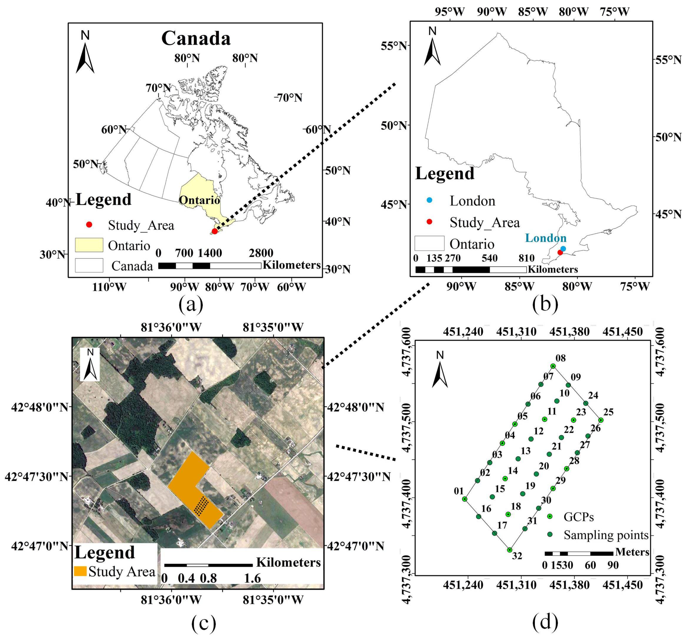
The study site was an agricultural production area located near London in the southwest of Ontario, Canada. The crop mix in this region mainly includes winter wheat, soybean, and corn. A part of the rectangular area of an “L-shaped” winter wheat planting area was selected for this study (Figure 1). The winter wheat in this region is generally sown in October of the previous year. During the winter months, winter wheat goes dormant, and resumes active growth in the spring. In May, the wheat grows rapidly and reaches maturity in mid and late July. Harvesting is usually done between late July and early August. For this study, multi-temporal ground measurements of LAI and the UAV RGB image acquisition were conducted from May to June 2019 of the wheat growing period.
2.2. Field Measurements
In this study, multi-temporal field measurements were conducted six times during May to June of the winter wheat growing period in 2019. A total of 32 sampling points were deployed along the row direction of winter wheat in the experimental field, and the distance between any 2 sampling points was no less than 30 m. The positions of each sampling point are shown in Figure 1d. In addition, to ensure the accuracy of relative positions between datasets, 12 sampling points were selected as ground control points, and 12 black-and-white chess boards (2 by 2 cells) measuring 1 ft by 1 ft were set up for subsequent data registration. The positions of each ground control point are shown in Figure 1d. At the same time the UAV was flown, LAI field measurement was carried out and a real-time kinematic (RTK) carrier phase division technology was used to record the longitude and latitude information of each sampling point. A Nikon D300S camera with a 10.5 mm fisheye lens was used to take 7 hemispherical photos of the winter wheat canopy at 1 m above the winter wheat canopy within a range of 2 m × 2 m at each sampling point. The field LAIe was derived by using CAN-EYE software to process hemispherical photos. The measured LAIe range was 0.31~0.67 on 11 May, 0.56~1.53 on 16 May, 0.75~2.52 on 21 May, 1.28~2.52 on 27 May, 1.11~1.8 on 3 June, and 1.52~2.3 on 11 June. On each measurement date, 32 samples were collected, resulting in a dataset of 192 samples from six measurement days.
2.3. UAV Data Acquisition and Processing
In the study, the DJI Phantom 4 RTK UAV system equipped with a 5 K high-resolution digital camera was used to collect RGB images on 2 May, 11 May, 16 May, 21 May, 27 May, 3 June, and 11 June 2019. All the UAV flights were performed between 10 a.m. and 2 p.m. and at an altitude of 30 m above the winter wheat canopy, with heading overlap and sideways overlap of 90%. The spatial resolution of the images obtained by UAV is 9 mm. The UAV image processing software Pix4Dmapper Pro V2.4 (Pix4D SA, Lausanne, Switzerland) was used to generate 3-D PCD including geometric information (x, y, z coordinate values) and optical information (RGB color components) of winter wheat using SfM technology. The SfM PCD was generated using a Windows computer with a 12-core Xeon CPU and Quadro M4000 graphics card, with a total processing time of 30 h. The PCD density is greater than 4000 points/m2.
2.4. Point Cloud Data Filtering
The gap fraction is the probability that the light passing through the canopy is not intercepted [38]. If only point cloud canopy data is not retained for point cloud data filtering, it will lead to an estimation error of gap fraction. Therefore, the separation of the bare ground point cloud and the winter wheat point cloud is very critical. PCD extracted from UAV images has both color information (red, green, and blue band values) and geometric information (x, y, and z coordinate values). The visible light vegetation index used for crop recognition in the visible light image can be applied to the extraction of vegetation points in the point cloud. Then, the Otsu method can be used to automatically determine the threshold to separate the ground points [39]. The Otsu method, also known as the maximum inter-class variance method, is a non-parametric and unsupervised method for automatic threshold selection [40]. The more common visible light vegetation index is the excess green index (EXG), which can be calculated by the following formula [39]:
where R, G, and B are the red, green, and blue band values of the digital image pixel acquired by the UAV, which are retained in the PCD generated by SfM.
The geometric information of PCD can be used to calculate the height difference and slope between nearby points. Vosselman proposed a slope-based filter that discriminates ground points by comparing slopes between a point and its neighbors [41]. A reasonable slope threshold can be obtained by using the data that contain the important terrain in the study area [42]. When winter wheat is greening up in the following spring, the coverage of winter wheat is very low. Most of the points in the PCD at this time represent the background soil, and reflect the terrain shape characteristics of the study area. Therefore, the PCD collected during this period can be used for obtaining the height difference threshold and slope threshold. Based on the approach mentioned above, the fixed threshold was improved to the height difference threshold set and slope threshold set based on the terrain characteristics of the study area, and an improved slope-based filtering algorithm was proposed. As shown in Figure 2, first divide the point cloud data area into grid data, and take the lowest point in each cell of grid data as the reference point, then calculate the height difference and slope value slope between the other points and the lowest point. The calculation formula is as follows:
where is the height difference between the lowest point and other points in the cell of grid data except the lowest point, is the z-coordinate value of , and is the z-coordinate value of .
where is the slope value of the other points in the cell of grid data except the lowest point, and are the x and y coordinate values of , and and are the x and y coordinate values of .
Then, use the average value of height difference and the average slope value of all points in a cell of grid data as the height difference threshold and slope threshold of the cell of grid data. Next, the height difference threshold set and slope threshold set can be obtained. In the subsequent point cloud filtering process, points with height differences less than the height difference threshold and slope less than the slope threshold will be filtered as ground points.
2.5. Projection of Spherical Point Cloud onto a Plane
The lens of the digital hemispherical photography system is a fisheye lens, which is also called a hemisphere lens. The view angle of the fisheye lens is close to or equal to . According to the imaging characteristics of the fisheye lens, the photosensitive part of the image is a circle, so a hemispherical photo is obtained [43]. In essence, a hemispherical photo produces a projection of a hemisphere onto a plane [44]. This study was based on the principle of measuring LAI using a digital hemispherical photography system. In order to obtain a hemispherical photo of a winter wheat field, the PCD of winter wheat needs be processed as follows. First, the PCD in the Cartesian coordinate system needs to be transformed into the spherical coordinate system, which projects the point cloud onto a hemispherical surface with a radius of one. Then, the point cloud on the hemispherical surface is projected onto a plane to obtain the gray hemispherical image of the point cloud. Next, the binary processing is performed by setting the gray value of the pixel with point cloud to 255 and the gray value of the pixel without point cloud to 0. Finally, the binary hemispherical image is obtained.
There are many ways to represent a sphere on a plane. In this study, two common projection methods, a Lambert azimuthal equal-area map projection and stereographic projection, were used [45]. The Lambert azimuthal equal-area map projection can keep the correct orientation from the projection center to any point and can keep the area on the map proportional to the corresponding area on the ground. The relationship between the coordinates before and after the projection is [36]:
where is any point on the sphere and is the projection of the point on the plane.
The stereographic projection is conformal. Conformality means that the angle remains unchanged. However, the projection does not maintain the same distance or area. The relationship between the coordinates before and after the projection is [36]:
where is any point on the sphere and is the projection of the point on the plane.
2.6. LAIe Estimation Using Gap Fraction
LAI is defined as the total of the one-sided leaf area per unit of ground surface area [2]. The LAI obtained under the assumption that leaf elements are randomly distributed in space is called the effective LAI (LAIe). LAIe is relatively easy to obtain from remote sensing data and can be mutually converted with the true LAI (LAI) () [19,46]. Therefore, many experiments often estimate the LAIe as a substitute for the true LAI [47]. When calculating LAIe, it is assumed that the leaf elements are randomly distributed in space (). Therefore, according to the Beer–Lambert law, the following equation can be obtained:
where is the zenith angle of the incident light, which refers to the angle between the light incident direction and the zenith direction. According to the mechanism of hemispherical photography, is the shooting angle. is the projection function, which is related to the zenith angle and the leaf inclination angle, and represents the projected area of the unit leaf under the view angle when the leaf inclination angle is α. is the gap fraction, which can be calculated by the following equation:
where is the pixel content of leaves under the viewing angle , and is the background (sky or soil) pixel content under the viewing angle .
When the zenith angle is , the projection function is independent of the leaf inclination angle and always equal to 0.5 [48]. Therefore, the zenith angle is substituted into Equation (6), and a single-angle inversion method can be obtained:
LAIe can also be estimated by gap fraction under different viewing angles, which is called the multi-angle inversion method:
where n is the number of divided concentric rings, is the gap fraction of the i-th concentric ring, and is the zenith angle difference between adjacent rings. The number of common concentric rings is 18, as shown in Figure 3. Since the hemispherical image contains information on the gap fraction from the to viewing angle, each concentric ring corresponds to a viewing angle interval. Under this condition, n is equal to 18, and is equal to in Equation (9). In Equation (8), can be approximated to the gap fraction of the viewing angle interval of the 12th concentric ring, and the corresponding viewing angle interval is .
According to two projection methods of spherical point cloud projecting onto a plane and two methods of calculating LAIe, four methods are combined to calculate LAIe. Combination 1 is the combination of the Lambert azimuthal equal-area map projection method and the single-angle inversion method, which is called the AEAP-SA method. Combination 2 is the combination of the Lambert azimuthal equal-area map projection method and the multi-angle inversion method, which is called the AEAP-MA method. Combination 3 is the combination of stereographic projection method and single angle inversion method, which is called the SP-SA method. Combination 4 is the combination of stereographic projection method and multi-angle inversion method, which is called the SP-MA method.
2.7. Methods Assessment
In this study, the in-site LAIe measurements were used to evaluate the accuracy of the LAIe derived from the UAV-based point cloud using different methods. Linear regression analysis was performed for estimated LAIe and LAIe was measured by DHP. The standard deviation (STD), determination coefficient (R2), root mean square error (RMSE), and average absolute error (MAE) were calculated to evaluate the prediction error of LAIe.
3. Results
3.1. Point Cloud Filtering
The Otsu filtering method and the Otsu filtering method combined with the improved slope-based filtering method were used, respectively, to separate the winter wheat point cloud and bare ground point cloud. Figure 4 shows the comparison diagram of filtering effects in local areas. It can be seen from the figure that on 11 May, 16 May, and 21 May, winter wheat was in the early growth stage, with less ground coverage and more bare ground. Due to the different weather and light at the time of photo shooting, the shadow effect of the picture was inconsistent, and the Otsu filtering method only used color information for filtering results in a small number of bare ground points that have not been removed. Combined with the improved slope-based filtering method, it improved the separation to a certain extent. However, with the rapid growth of winter wheat, winter wheat covered more and more ground, leaving less bare ground. Using an improved slope-based filtering algorithm will filter out a small portion of the winter wheat point cloud.
3.2. Hemispherical Image of Point Cloud Data
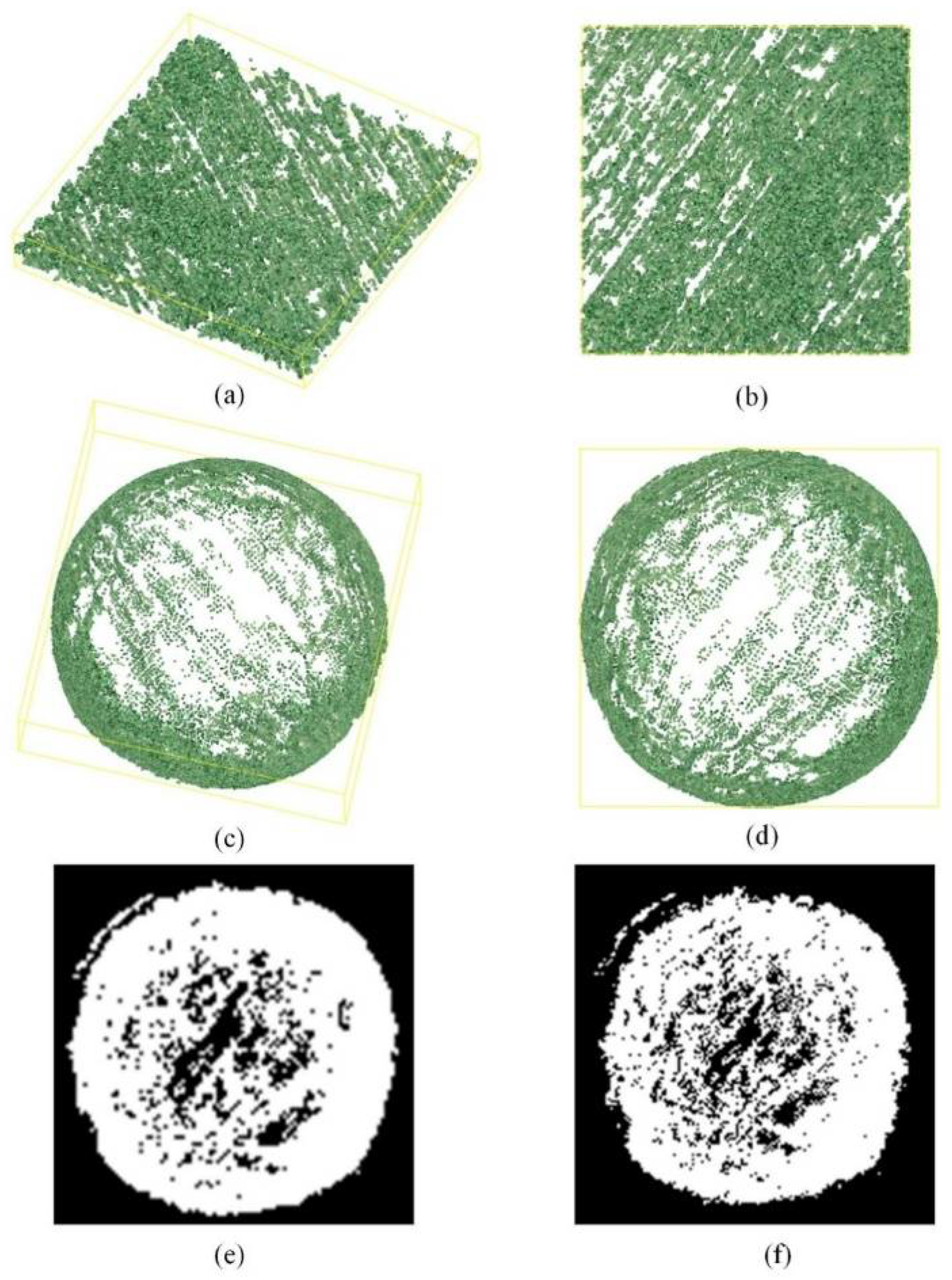
The filtered winter wheat point cloud data was projected onto a hemispherical surface, and the hemispherical image was then obtained through the Lambert azimuthal equal-area map projection and the stereographic projection and binarization, respectively. In the binary hemispherical image, the white pixels represent the winter wheat point cloud, and the black pixels represent soil ground points. The winter wheat point cloud data before and after projection and the binary hemispherical image are shown in Figure 5. The Lambert azimuthal equal-area map projection does not guarantee the angle, and the area of any area on the sphere projected onto the projection plane is equal in proportion. The stereographic projection does not preserve the area but the angle. The closer to the equator, the larger the area is. Therefore, when the spherical point cloud is projected to the plane using stereographic projection, the smaller the latitude line is, the larger the proportion of the projected area is. This can be seen from Figure 5e,f.
3.3. LAIe Inversion Results
Figure 6, Figure 7, Figure 8 and Figure 9 show the regression analysis results between the LAIe estimated using the four methods under three filtering conditions and the LAIe measured by DHP. Without filtering, the LAIe estimated based on UAV PCD using the AEAP-SA method and SP-SA method is negatively correlated with the LAIe measured by DHP (Figure 6a and Figure 8a). Without filtering, the LAIe estimated based on the UAV point cloud data using the AEAP-MA method and SP-MA method is weakly correlated with the LAIe measured by the DHP (Figure 7a and Figure 9a). Under the other two filtering conditions, the LAIe estimated by the four methods based on UAV point cloud data is positively correlated with the LAIe measured by ground DHP (Figure 7, Figure 8, Figure 9 and Figure 10). The STD, RMSE, MAE, and R2 of LAIe estimated by four methods under three filtering conditions are listed in Table 1, Table 2, Table 3 and Table 4.
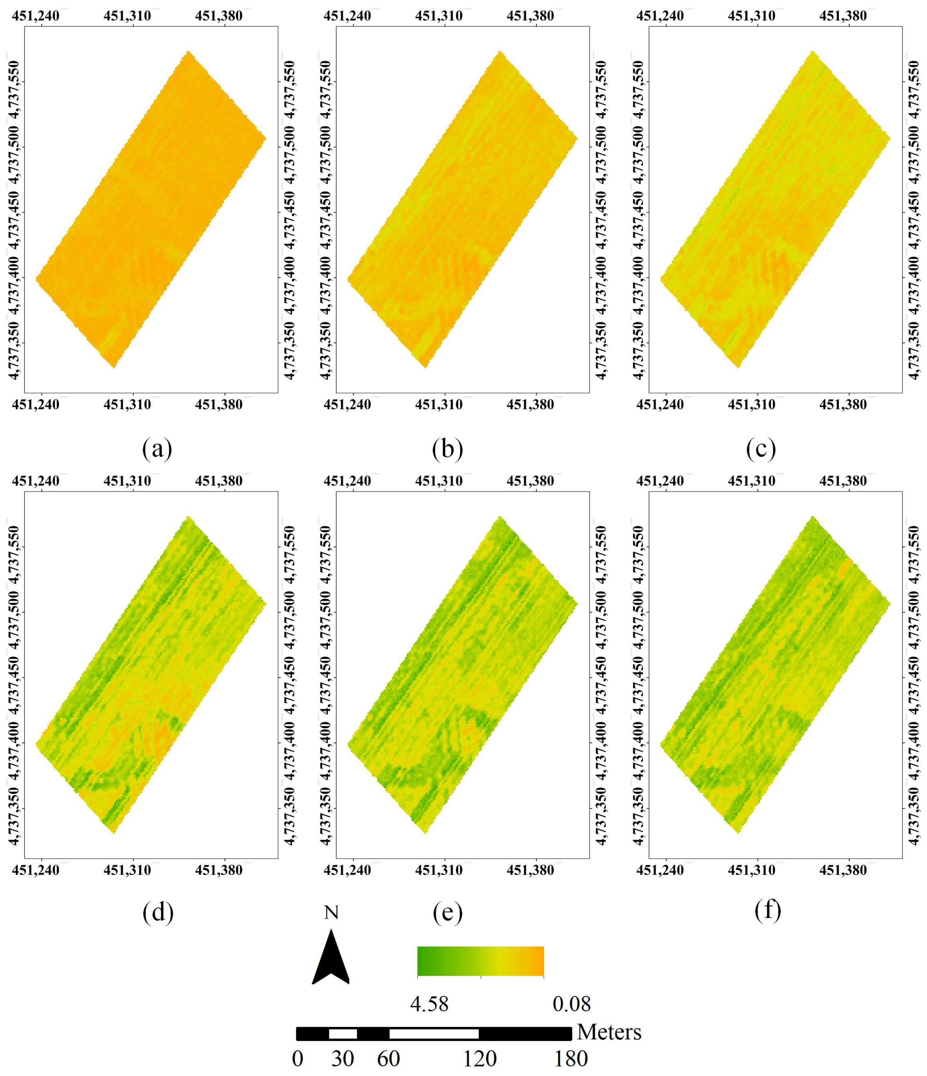
When the Otsu filtering method is used in combination with the improved slope-based filtering method, the LAIe values of enough sampling points in the study area were estimated by four methods and the LAIe maps are drawn in Figure 10, Figure 11, Figure 12 and Figure 13.
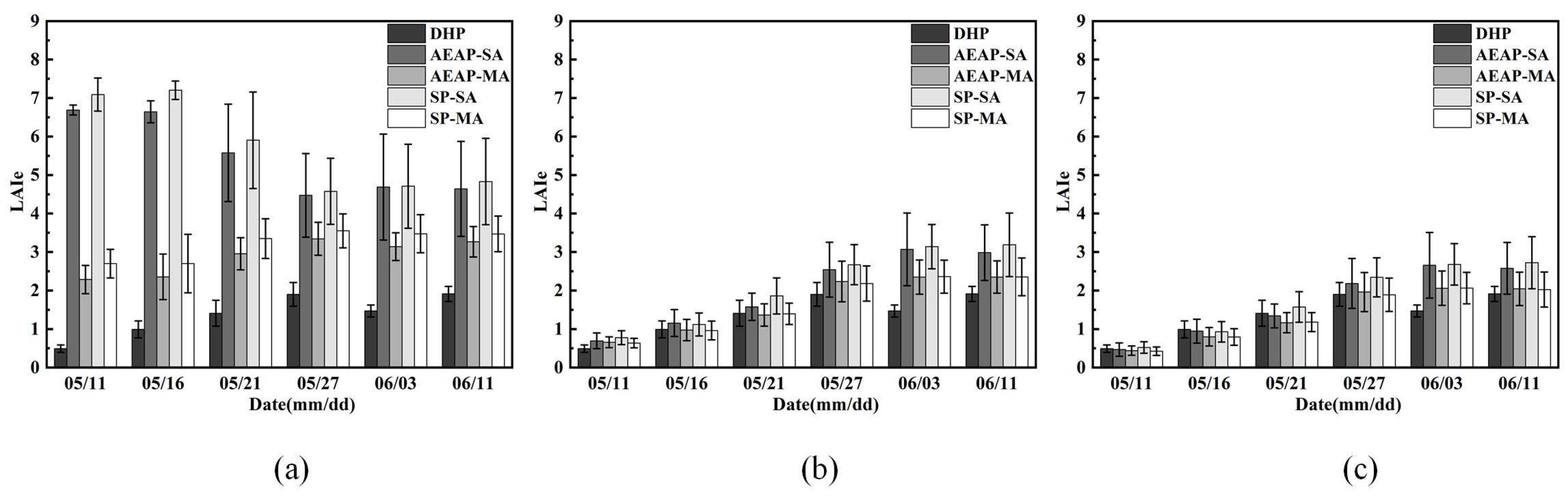
Using the mean LAIe measured by DHP and estimated by four methods as data points, and the STD as error bars, the bar charts with error bars were drawn to explore the uncertainty of the four methods compared with the DHP method (Figure 14). These three conditions and four methods mentioned above to estimate the LAIe are compared and discussed below.
4. Discussion
4.1. Accuracy Comparison of LAIe Estimation by Filtering Methods
Without filtering, the LAIe obtained by four methods of estimating LAIe based on UAV point cloud data were weakly or negatively correlated with the LAIe measured by ground DHP, and the RMSE and MAE were relatively large (Table 1, Table 2, Table 3 and Table 4). It can be seen that it was very necessary to filter the point cloud data and separate the winter wheat point cloud from the bare ground point cloud. This is because there was no filter to separate the winter wheat point cloud and the bare ground point cloud, and the white pixel value of the binary hemispherical image contained a large amount of bare ground point cloud. The bare ground point cloud was regarded as the winter wheat point cloud, which caused the calculated gap fraction to be low. Therefore, the LAIe obtained would be seriously overestimated, which is particularly obvious in the early growth stage of winter wheat (Figure 6, Figure 7, Figure 8 and Figure 9). As shown in Figure 6a, Figure 7a, Figure 8a and Figure 9a, on 11, 16, and 21 May, winter wheat covered less ground, and bare ground point cloud accounted for most of the point cloud data, which made the estimated LAIe value much higher than the measured LAIe value. At the late growth stage of winter wheat, such as 3 June and 11 June, the amount of point cloud on the bare ground was relatively small, and the situation regarding the LAIe estimation being on the high side was improved.
Compared with forest point cloud and individual tree point cloud, the height of winter wheat is relatively low, and the influence of terrain should be considered, so it is much more complex to filter winter wheat point cloud. When only Otsu filtering was used, this paper calculated the color index EXG based on RGB pixel information about point cloud data, and then automatically determined the threshold value of EXG using the Otsu method to separate winter wheat point cloud from background soil point cloud. The Otsu method divides the point cloud into foreground and background according to the EXG of the point cloud data, and then selects the best EXG value to maximize the variance between the foreground and background, so as to automatically determine the threshold. In the case of different lighting conditions, i.e., uneven light and shadows, the EXG of some bare ground point cloud was similar to the EXG of winter wheat point cloud, and some bare ground point cloud may have been mistaken for winter wheat point cloud and retained. Therefore, when only the Otsu filtering method was used, the estimated value of the LAIe is on the high side. Song et al. also showed that shadow effect is one of the factors that affect the estimation of LAIe [39].
In addition to color information, point cloud data also has geometric information. According to the structure information of point cloud data, this paper proposed an improved slope-based filtering method. Combining this method with the Otsu filtering method, background soil points could be better separated. The correlation between estimated LAIe and the LAIe measured by DHP was improved, and MAE and RMSE were decreased when the Otsu filtering method was combined with the improved slope-based filtering method (Table 1, Table 2, Table 3 and Table 4). At the early growing stage, winter wheat covered less ground, and there were fewer winter wheat point clouds after Otsu filtering. When using the improved slope-based filtering method, if the lowest point in a grid is a winter wheat point cloud, part of the winter wheat point cloud in the grid will be filtered out, which will cause the LAIe estimation value to be lower than the LAIe measurement value. In the late growth stage of winter wheat, with the increase of winter wheat point cloud, this situation is improved. In a word, when using the Otsu filtering method in combination with the improved slope-based filtering method, compared with using only the Otsu filtering method, the problem that some bare ground points are not filtered out, resulting in higher LAIe estimates, has improved to some extent, but also led to lower LAIe estimates at the early growing stage of winter wheat. This is where further improvement is needed in the future. The improved sloped-based algorithm needs to use point cloud data at the early growing stage of the crop to calculate the height difference threshold set and slope threshold set. In future studies, the height difference threshold set and slope threshold set can be calculated by using the digital elevation model (DEM) generated by point cloud to make the classification of crop point cloud and bare ground point cloud more accurate.
From the inversion results of LAIe, it can be seen that the inversion value of LAIe is much higher than the measured value when the bare ground points are not filtered. In the two cases where the bare ground points were filtered, the inversion value of LAIe is close to but still slightly higher than the measured value as a whole. The above bare ground point cloud is regarded as the winter wheat point cloud, which leads to an underestimated gap fraction. In addition, the research of Danson et al. showed that the method based on TLS often underestimates the gap fraction [38], and the results of the gap fraction estimated by Hancock et al. from the PCD based on TLS through the two-dimensional method were consistent with it [37]. Zheng et al. further confirmed this finding, indicating that the LAIe obtained from the PCD based on TLS using the two-dimensional method was overestimated [36]. The results of this study are consistent with the above results.
4.2. Assessment of Four Methods for LAIe Estimation
According to Table 1, Table 2, Table 3 and Table 4, compared with the DHP method, the AEAP-MA method and SP-MA method have higher R2 and lower RMSE and MAE than those of the AEAP-SA method and SP-SA method. The RMSE and MAE of the AEAP-SA method and SP-SA method in the late growth stage of winter wheat (27 May, 3 June, and 21 June) were much higher than those in the early growth stage of winter wheat (11 May, 16 May, and 21 May), which resulted in higher overall errors (Table 1, Table 2, Table 3 and Table 4). Among the four methods, the R2 of the SP-MA method was the highest, and the RMSE and MAE were the lowest. The uncertainty of the AEAP-MA method and SP-MA method is relatively small, while the uncertainty of the AEAP-SA method and SP-SA method are relatively large (Figure 14). In addition, the Kruskal–Wallis analysis of variance for the nonparametric test of absolute error of the four methods was conducted. Table 5 lists the p-values of the significance analysis of absolute error distribution of the different methods. The absolute error distribution of the SP-MA method is significantly different from that of the AEAP-SA method and SP-SA method (p < 0.01). It can be considered that the absolute error of the SP-MA method is significantly lower than that of the AEAP-SA method and SP-SA method. The absolute error distribution of the SP-MA method and AEAP-MA method is not significantly different. The SP-MA method has the highest R2 and the lowest MAE and RMSE, indicating that it has the highest estimation accuracy among the four methods.
First, we discuss the influence of Lambert azimuthal equal-area map projection and stereographic projection on the LAIe estimation. It can be seen from Figure 4 that when the point cloud data was projected onto the upper hemisphere, the winter wheat point cloud was mainly concentrated in the regions with lower spherical latitude, whereas the bare ground point cloud was mainly distributed in the poles and regions with higher latitude. As mentioned earlier, Lambert azimuthal equal-area map projection preserves area but not angle, whereas stereographic projection preserves angle but not area. That is to say, after the Lambert azimuthal equal-area map projection, the area of any latitude area on the sphere is projected in equal proportion; after the stereographic projection, the lower the latitude on the sphere, the larger the projected area. Because the winter wheat point cloud data was mainly concentrated in the area with lower spherical latitude, the area with lower latitude was enlarged after using the stereographic projection, and the distribution details of the winter wheat point cloud were better displayed. Therefore, under the stereographic projection, the calculation of gap fraction was more accurate. This agrees with the research results of Zheng et al. Zheng et al. used the two-dimensional method to convert the PCD into a two-dimensional raster image to estimate the LAIe of a forest stand, and the stereographic projection method correlated better to the DHP-based LAIe compared with the Lambert azimuthal equal-area map projection method [36]. However, this study only selected these two more commonly used projection methods of spherical point cloud onto a plane; other projection methods such as polar projection and orthogonal projection can be tried.
Since the single-angle inversion method only uses the gap fraction of concentric rings in the viewing angle area to estimate LAIe, the concentric rings in this viewing angle area were just the concentrated area of winter wheat point cloud. The multi-angle inversion method uses the gap fraction of 18 concentric rings to estimate the LAIe, and calculates the gap fraction of all viewing areas to estimate the LAIe. This explains why the LAIe value estimated by the single-angle inversion method is higher than that estimated by the multi-angle inversion method. The extracted gap fraction information by the multi-angle inversion method is more comprehensive, so the estimated LAIe value is more relevant to the DHP-based LAIe. This is in agreement with the research results of Song et al., who developed a method of simulated observation of point cloud (SOPC) from a three-dimensional perspective based on UAV point cloud data to obtain the gap fraction under the corresponding zenith angle, and then retrieved the LAIe from a single angle and multiple angles, respectively [39]. Overall, the SP-MA method is the combination of the stereographic projection and multi-angle inversion method, which allows a more comprehensive consideration of the canopy information of winter wheat point cloud, so the accuracy of LAIe value estimated by this method is the highest.
5. Conclusions
In this paper, we used four methods of simulated hemispherical photography to estimate the LAIe from UAV-based PCD, and discussed the impact of different filtering methods on the LAIe estimation results. The results show that the LAIe estimated by the four methods of estimating LAIe are moderately and strongly correlated with the LAIe measured by DHP. Among them, the combination of stereographic projection and multi-angle inversion method has the highest accuracy, with a R2 of 0.63. In addition, the effect of filtering PCD to separate winter wheat point cloud and the background soil point cloud has an important impact on LAIe estimation. The improved slope-based filtering method proposed in this study combined with the Otsu filtering method can improve the estimation accuracy of LAIe. Overall, the PCD processing routines applied in this paper could be automated, and the method proposed in this study could conveniently and effectively estimate the LAIe of crops in larger areas using UAV-based 3-D PCD without ground measurement.
Author Contributions
Data curation, Y.S., J.W. and M.X. (Minfeng Xing); investigation, J.Y.; methodology, M.X. (Minfeng Xing) and J.Y.; supervision, J.W. and M.X. (Minfeng Xing); validation, J.Y., M.X. (Min Xu) and Q.T.; writing—original draft, J.Y. and M.X. (Minfeng Xing); writing—review and editing, J.Y., M.X. (Minfeng Xing), Q.T., J.S., Y.S., X.N., J.W. and M.X. (Min Xu); All authors have read and agreed to the published version of the manuscript.
Funding
This work was supported by the National Natural Science Foundation of China, grant numbers 41601373 and U20A2090; the Scientific Research Starting Foundation from the Yangtze Delta Region Institute (Huzhou), and the University of Electronic Science and Technology of China, grant number U03210022.
Institutional Review Board Statement
Not applicable.
Informed Consent Statement
Not applicable.
Data Availability Statement
Not applicable.
Conflicts of Interest
The authors declare no conflict of interest.
References
- Weiss, M.; Baret, F.; Smith, G.; Jonckheere, I.; Coppin, P. Review of methods for in situ leaf area index (LAI) determination: Part II. Estimation of LAI, errors and sampling. Agric. For. Meteorol. 2004, 121, 37–53. [Google Scholar] [CrossRef]
- Fang, H.L.; Baret, F.; Plummer, S.; Schaepman-Strub, G. An Overview of Global Leaf Area Index (LAI): Methods, Products, Validation, and Applications. Rev. Geophys. 2019, 57, 739–799. [Google Scholar] [CrossRef]
- Luisa, E.M.; Frederic, B.; Marie, W. Slope correction for LAI estimation from gap fraction measurements. Agric. For. Meteorol. 2008, 148, 1553–1562. [Google Scholar] [CrossRef]
- Nackaerts, K.; Coppin, P.; Muys, B.; Hermy, M. Sampling methodology for LAI measurements with LAI-2000 in small forest stands. Agric. For. Meteorol. 2000, 101, 247–250. [Google Scholar] [CrossRef]
- Denison, R.F.; Russotti, R. Field estimates of green leaf area index using laser-induced chlorophyll fluorescence. Field Crops Res. 1997, 52, 143–149. [Google Scholar] [CrossRef]
- Denison, R. Minimizing errors in LAI estimates from laser-probe inclined-point quadrats. Field Crops Res. 1997, 51, 231–240. [Google Scholar] [CrossRef]
- Garrigues, S.; Shabanov, N.V.; Swanson, K.; Morisette, J.T.; Baret, F.; Myneni, R.B. Intercomparison and sensitivity analysis of Leaf Area Index retrievals from LAI-2000, AccuPAR, and digital hemispherical photography over croplands. Agric. For. Meteorol. 2008, 148, 1193–1209. [Google Scholar] [CrossRef]
- Jiapaer, G.; Yi, Q.X.; Yao, F.; Zhang, P. Comparison of non-destructive LAI determination methods and optimization of sampling schemes in Populus euphratica. Urban For. Urban Green. 2017, 26, 114–123. [Google Scholar] [CrossRef]
- Yan, G.J.; Hu, R.H.; Luo, J.H.; Weiss, M.; Jiang, H.L.; Mu, X.H.; Xie, D.H.; Zhang, W.M. Review of indirect optical measurements of leaf area index: Recent advances, challenges, and perspectives. Agric. For. Meteorol. 2019, 265, 390–411. [Google Scholar] [CrossRef]
- Kussner, R.; Mosandl, R. Comparison of direct and indirect estimation of leaf area index in mature Norway spruce stands of eastern Germany. Can. J. For. Res. 2000, 30, 440–447. [Google Scholar] [CrossRef]
- Rhoads, A.G.; Hamburg, S.P.; Fahey, T.J.; Siccama, T.G.; Kobe, R. Comparing direct and indirect methods of assessing canopy structure in a northern hardwood forest. Can. J. For. Res. 2004, 34, 584–591. [Google Scholar] [CrossRef]
- Jay, S.; Maupas, F.; Bendoula, R.; Gorretta, N. Retrieving LAI, chlorophyll and nitrogen contents in sugar beet crops from multi-angular optical remote sensing: Comparison of vegetation indices and PROSAIL inversion for field phenotyping. Field Crops Res. 2017, 210, 33–46. [Google Scholar] [CrossRef]
- Chen, Y.; Zhang, Z.; Tao, F.L. Improving regional winter wheat yield estimation through assimilation of phenology and leaf area index from remote sensing data. Eur. J. Agron. 2018, 101, 163–173. [Google Scholar] [CrossRef]
- Zhang, P.; Anderson, B.; Tan, B.; Huang, D.; Myneni, R. Potential monitoring of crop production using a new satellite-Based Climate-Variability Impact Index. Agric. For. Meteorol. 2005, 132, 344–358. [Google Scholar] [CrossRef]
- Huang, J.X.; Tian, L.Y.; Liang, S.L.; Ma, H.Y.; Becker-Reshef, I.; Huang, Y.B.; Su, W.; Zhang, X.D.; Zhu, D.H.; Wu, W.B. Improving winter wheat yield estimation by assimilation of the leaf area index from Landsat TM and MODIS data into the WOFOST model. Agric. For. Meteorol. 2015, 204, 106–121. [Google Scholar] [CrossRef]
- Song, Y.; Wang, J.F.; Shan, B. Estimation of winter wheat yield from UAV-based multi-temporal imagery using crop allometric relationship and SAFY model. Drones 2021, 5, 78. [Google Scholar] [CrossRef]
- Luo, S.Z.; Chen, J.M.; Wang, C.; Gonsamo, A.; Xi, X.H.; Lin, Y.; Qian, M.J.; Peng, D.L.; Nie, S.; Qin, H.M. Comparative performances of airborne LiDAR height and intensity data for leaf area index estimation. IEEE J. Sel. Topics Appl. Earth Observ. Remote Sens. 2017, 11, 300–310. [Google Scholar] [CrossRef]
- Maki, M.; Homma, K. Empirical Regression Models for Estimating Multiyear Leaf Area Index of Rice from Several Vegetation Indices at the Field Scale. Remote Sens. 2014, 6, 4764–4779. [Google Scholar] [CrossRef]
- Liu, K.; Zhou, Q.B.; Wu, W.B.; Xia, T.; Tang, H.J. Estimating the crop leaf area index using hyperspectral remote sensing. J. Integr. Agric. 2016, 15, 475–491. [Google Scholar] [CrossRef]
- Yuan, H.H.; Yang, G.J.; Li, C.C.; Wang, Y.J.; Liu, J.G.; Yu, H.Y.; Feng, H.K.; Xu, B.; Zhao, X.Q.; Yang, X.D. Retrieving Soybean Leaf Area Index from Unmanned Aerial Vehicle Hyperspectral Remote Sensing: Analysis of RF, ANN, and SVM Regression Models. Remote Sens. 2017, 9, 309. [Google Scholar] [CrossRef]
- Tang, H.; Brolly, M.; Zhao, F.; Strahler, A.H.; Schaaf, C.L.; Ganguly, S.; Zhang, G.; Dubayah, R. Deriving and validating Leaf Area Index (LAI) at multiple spatial scales through lidar remote sensing: A case study in Sierra National Forest, CA. Remote Sens. Environ. 2014, 143, 131–141. [Google Scholar] [CrossRef]
- Duan, B.; Liu, Y.T.; Gong, Y.; Peng, Y.; Wu, X.T.; Zhu, R.S.; Fang, S.H. Remote estimation of rice LAI based on Fourier spectrum texture from UAV image. Plant Methods 2019, 15, 124. [Google Scholar] [CrossRef] [PubMed]
- Qi, J.; Kerr, Y.H.; Moran, M.S.; Weltz, M.; Huete, A.R.; Sorooshian, S.; Bryant, R. Leaf Area Index Estimates Using Remotely Sensed Data and BRDF Models in a Semiarid Region. Remote Sens. Environ. 2000, 73, 18–30. [Google Scholar] [CrossRef]
- Tian, Y.; Huang, H.; Zhou, G.; Zhang, Q.; Tao, J.; Zhang, Y.; Lin, J. Aboveground mangrove biomass estimation in Beibu Gulf using machine learning and UAV remote sensing. Sci.Total Environ. 2021, 781, 146816. [Google Scholar] [CrossRef]
- Tian, J.Y.; Wang, L.; Li, X.J.; Gong, H.L.; Shi, C.; Zhong, R.F.; Liu, X.M. Comparison of UAV and WorldView-2 imagery for mapping leaf area index of mangrove forest. Int. J. Appl. Earth Observation GeoInf. 2017, 61, 22–31. [Google Scholar] [CrossRef]
- Li, S.Y.; Yuan, F.; Ata-UI-Karim, S.T.; Zheng, H.B.; Cheng, T.; Liu, X.J.; Tian, Y.C.; Zhu, Y.; Cao, W.X.; Cao, Q. Combining Color Indices and Textures of UAV-Based Digital Imagery for Rice LAI Estimation. Remote Sens. 2019, 11, 1763. [Google Scholar] [CrossRef]
- Liu, S.B.; Jin, X.; Nie, C.W.; Wang, S.Y.; Yu, X.; Cheng, M.H.; Shao, M.C.; Wang, Z.X.; Tuohuti, N.; Bai, Y.; et al. Estimating leaf area index using unmanned aerial vehicle data: Shallow vs. deep machine learning algorithms. Plant Physiol. 2021, 187, 1551–1576. [Google Scholar] [CrossRef]
- Duan, S.B.; Li, Z.L.; Wu, H.; Tang, B.H.; Ma, L.L.; Zhao, E.Y.; Li, C.R. Inversion of the PROSAIL model to estimate leaf area index of maize, potato, and sunflower fields from unmanned aerial vehicle hyperspectral data. Int. J. Appl. Earth Obs. GeoInf. 2014, 26, 12–20. [Google Scholar] [CrossRef]
- Pascu, I.; Dobre, A.; Badea, O.; Tanase, M. Estimating forest stand structure attributes from terrestrial laser scans. Sci. Total Environ. 2019, 691, 205–215. [Google Scholar] [CrossRef]
- dos Santos, L.M.; Ferraz, G.A.E.S.; Barbosa, B.D.D.; Diotto, A.V.; Maciel, D.T.; Xavier, L.A.G. Biophysical parameters of coffee crop estimated by UAV RGB images. Precis. Agric. 2020, 21, 1227–1241. [Google Scholar] [CrossRef]
- Wallace, L.; Lucieer, A.; Malenovsky, Z.; Turner, D.; Vopenka, P. Assessment of forest structure using two UAV techniques: A comparison of airborne laser scanning and structure from motion (SfM) point clouds. Forests 2016, 7, 62. [Google Scholar] [CrossRef]
- Arno, J.; Escola, A.; Valles, J.M.; Llorens, J.; Sanz, R.; Masip, J.; Palacin, J.; Rosell-Polo, J.R. Leaf area index estimation in vineyards using a ground-based LiDAR scanner. Precis. Agric. 2013, 14, 290–306. [Google Scholar] [CrossRef]
- Comba, L.; Biglia, A.; Aimonino, D.R.; Tortia, C.; Mania, E.; Guidoni, S.; Gay, P. Leaf Area Index evaluation in vineyards using 3D point clouds from UAV imagery. Precis. Agric. 2020, 21, 881–896. [Google Scholar] [CrossRef]
- Yin, T.G.; Qi, J.B.; Cook, B.D.; Morton, D.C.; Wei, S.S.; Gastellu-Etchegorry, J.-P. Modeling small-footprint airborne LiDAR-derived estimates of gap probability and leaf area index. Remote Sens. 2019, 12, 4. [Google Scholar] [CrossRef]
- Ross, C.W.; Loudermilk, E.L.; Skowronski, N.; Pokswinski, S.; Hiers, J.K.; O’Brien, J. LiDAR Voxel-Size Optimization for Canopy Gap Estimation. Remote Sens. 2022, 14, 1054. [Google Scholar] [CrossRef]
- Zheng, G.; Moskal, L.M.; Kim, S.-H. Retrieval of Effective Leaf Area Index in Heterogeneous Forests With Terrestrial Laser Scanning. IEEE Trans. Geosci. 2013, 51, 777–786. [Google Scholar] [CrossRef]
- Hancock, S.; Essery, R.; Reild, T.; Carle, J.; Baxter, R.; Rutter, N.; Huntley, B. Characterising forest gap fraction with terrestrial lidar and photography: An examination of relative limitations. Agric. For. Meteorol. 2014, 189, 105–114. [Google Scholar] [CrossRef]
- Danson, F.M.; Hetherington, D.; Morsdorf, F.; Koetz, B.; Allgower, B. Forest canopy gap fraction from terrestrial laser scanning. IEEE Geosci. Remote Sens. Lett. 2007, 4, 157–160. [Google Scholar] [CrossRef]
- Song, Y.; Wang, J.F.; Shang, J.L. Estimating effective leaf area index of winter wheat using simulated observation on unmanned aerial vehicle-based point cloud data. IEEE J. Sel. Topics Appl. Earth Observ. Remote Sens. 2020, 13, 2874–2887. [Google Scholar] [CrossRef]
- Otsu, N. A threshold selection method from gray-level histograms. IEEE Trans. Syst. Man Cybern. 1979, 9, 62–66. [Google Scholar] [CrossRef]
- Vosselman, G. Slope based filtering of laser altimetry data. IAPRS 2000, 18, 935–942. [Google Scholar]
- Zhang, K.Q.; Chen, S.C.; Whitman, D.; Shyu, M.L.; Yan, J.H.; Zhang, C.C. A progressive morphological filter for removing nonground measurements from airborne LIDAR data. IEEE Trans. Geosci. Remote Sens. Environ. 2003, 41, 872–882. [Google Scholar] [CrossRef]
- Herbert, T.J. Calibration of fisheye lenses by inversion of area projections. Appl. Opt. 1986, 25, 1875–1876. [Google Scholar] [CrossRef] [PubMed]
- Jonckheere, I.; Fleck, S.; Nackaerts, K.; Muys, B.; Coppin, P.; Weiss, M.; Baret, F. Review of methods for in situ leaf area index determination: Part I. Theories, sensors and hemispherical photography. Agric. For. Meteorol. 2004, 121, 19–35. [Google Scholar] [CrossRef]
- Herbert, T.J. Area projections of fisheye photographic lenses. Agric. For. Meteorol. 1987, 39, 215–223. [Google Scholar] [CrossRef]
- Zheng, G.; Moskal, L.M. Computational-Geometry-Based Retrieval of Effective Leaf Area Index Using Terrestrial Laser Scanning. IEEE Trans. Geosci. Remote Sens. 2012, 50, 3958–3969. [Google Scholar] [CrossRef]
- Heiskanen, J.; Korhonen, L.; Hietanen, J.; Pellikka, P. Use of airborne lidar for estimating canopy gap fraction and leaf area index of tropical montane forests. Int. J. Remote Sens. 2015, 36, 2569–2583. [Google Scholar] [CrossRef]
- Chen, J.M.; Menges, C.H.; Leblanc, S.G. Global mapping of foliage clumping index using multi-angular satellite data. Remote Sens. Environ. 2005, 97, 447–457. [Google Scholar] [CrossRef]
Figure 1.
Location of the study area and sampling points. (a) Study area in Ontario, Canada. (b) Study area located near London in southwestern Ontario. (c) Study area of “L-shaped” winter wheat field. (d) Locations of sampling points and ground control points (GCPs) within the winter wheat field.
Figure 1.
Location of the study area and sampling points. (a) Study area in Ontario, Canada. (b) Study area located near London in southwestern Ontario. (c) Study area of “L-shaped” winter wheat field. (d) Locations of sampling points and ground control points (GCPs) within the winter wheat field.

Figure 2.
Schematic diagram of grid data and calculation of height difference and slope value. (a) Divide the point cloud data area into grid data (top view). (b) Calculation of height difference and distance in a cell of grid data, where and .
Figure 2.
Schematic diagram of grid data and calculation of height difference and slope value. (a) Divide the point cloud data area into grid data (top view). (b) Calculation of height difference and distance in a cell of grid data, where and .

Figure 3.
Division of hemispherical image view angles into 18 rings (18 views). In this hemispherical image, green represents leaf pixels and white represents non-leaf pixels.
Figure 3.
Division of hemispherical image view angles into 18 rings (18 views). In this hemispherical image, green represents leaf pixels and white represents non-leaf pixels.

Figure 4.
Schematic diagram of the filtering effect. (a,d,g,j,m,p) show the original point cloud on 11 May, 16 May, 21 May, 26 May, 3 June, and 11 June. (b,e,h,k,n,q) show the point cloud on 11 May, 16 May, 21 May, 26 May, 3 June, and 11 June filtered by the Otsu method. (c,f,i,l,o,r) show the point cloud on 11 May, 16 May, 21 May, 26 May, 3 June, and 11 June after using the Otsu filtering method in combination with the improved slope-based filtering method.

Figure 5.
Project the point cloud data in the 3-D Cartesian coordinate system to the upper hemisphere, then project it to the plane and binarize it to obtain the hemispherical image (The yellow box is the bounding box of the point cloud). (a) is the point cloud in the 3-D Cartesian coordinate system. (b) is the top view of the point cloud in the 3-D Cartesian coordinate system. (c) is the point cloud in the spherical coordinate system. (d) is the top view of the point cloud in the spherical coordinate system. (e) is the binary hemispherical image obtained by the Lambert azimuthal equal-area map projection method. (f) is the binary hemispherical image obtained by the stereographic projection method.

Figure 6.
Linear regression analysis of LAIe calculated by the AEAP-SA method and LAIe measured by DHP under different filtering conditions. (a) is the case without filtering. (b) is the case only using the Otsu filtering method. (c) is the case using the Otsu filtering method combined with improved slope-based filtering method. Six sample points with different dates are represented in different colors to distinguish them. Among them, black represents 32 sampling points on 11 May, red represents 32 sampling points on 16 May, blue represents 32 sampling points on 21 May, green represents 32 sampling points on 27 May, purple represents 32 sampling points on 3 June, and yellow represents 32 sampling points on 11 June. The solid line is a linear regression trend line, and the dotted line is the 1:1 line.

Figure 7.
Linear regression analysis of LAIe calculated by the AEAP-MA method and LAIe measured by DHP under different filtering conditions. (a) is the case without filtering. (b) is the case only using the Otsu filtering method. (c) is the case using the Otsu filtering method combined with improved slope-based filtering method. Six sampling points with different dates are represented in different colors to distinguish them. Among them, black represents 32 sampling points on 11 May, red represents 32 sampling points on 16 May, blue represents 32 sampling points on 21 May, green represents 32 sampling points on 27 May, purple represents 32 sampling points on 3 June, and yellow represents 32 sampling points on 11 June. The solid line is a linear regression trend line, and the dotted line is the 1:1 line.

Figure 8.
Linear regression analysis of LAIe calculated by the SP-SA method and LAIe measured by DHP under different filtering conditions. (a) is the case without filtering. (b) is the case only using the Otsu filtering method. (c) is the case using the Otsu filtering method combined with improved slope-based filtering method. Six sampling points with different dates are represented in different colors to distinguish them. Among them, black represents 32 sampling points on 11 May, red represents 32 sampling points on 16 May, blue represents 32 sampling points on 21 May, green represents 32 sampling points on 27 May, purple represents 32 sampling points on 3 June, and yellow represents 32 sampling points on 11 June. The solid line is a linear regression trend line, and the dotted line is the 1:1 line.

Figure 9.
Linear regression analysis of LAIe calculated by the SP-MA method and LAIe measured by DHP under different filtering conditions. (a) is the case without filtering. (b) is the case only using the Otsu filtering method. (c) is the case using the Otsu filtering method combined with improved slope-based filtering method. Six sampling points with different dates are represented in different colors to distinguish them. Among them, black represents 32 sampling points on 11 May, red represents 32 sampling points on 16 May, blue represents 32 sampling points on 21 May, green represents 32 sampling points on 27 May, purple represents 32 sampling points on 3 June, and yellow represents 32 sampling points on 11 June. The solid line is a linear regression trend line, and the dotted line is the 1:1 line.

Figure 10.
LAIe of six dates generated based on the UAV 3-D point cloud dataset using the AEAP-SA method: (a) 11 May; (b) 16 May; (c) 21 May; (d) 27 May; (e) 3 June; (f) 11 June.
Figure 10.
LAIe of six dates generated based on the UAV 3-D point cloud dataset using the AEAP-SA method: (a) 11 May; (b) 16 May; (c) 21 May; (d) 27 May; (e) 3 June; (f) 11 June.

Figure 11.
LAIe of six dates generated based on the UAV 3-D point cloud dataset using the AEAP-MA method: (a) 11 May; (b) 16 May; (c) 21 May; (d) 27 May; (e) 3 June; (f) 11 June.
Figure 11.
LAIe of six dates generated based on the UAV 3-D point cloud dataset using the AEAP-MA method: (a) 11 May; (b) 16 May; (c) 21 May; (d) 27 May; (e) 3 June; (f) 11 June.

Figure 12.
LAIe of six dates generated based on the UAV 3-D point cloud dataset using the SP-SA method: (a) 11 May; (b) 16 May; (c) 21 May; (d) 27 May; (e) 3 June; (f) 11 June.
Figure 12.
LAIe of six dates generated based on the UAV 3-D point cloud dataset using the SP-SA method: (a) 11 May; (b) 16 May; (c) 21 May; (d) 27 May; (e) 3 June; (f) 11 June.

Figure 13.
LAIe of six dates generated based on the UAV 3-D point cloud dataset using the SP-MA method: (a) 11 May; (b) 16 May; (c) 21 May; (d) 27 May; (e) 3 June; (f) 11 June.
Figure 13.
LAIe of six dates generated based on the UAV 3-D point cloud dataset using the SP-MA method: (a) 11 May; (b) 16 May; (c) 21 May; (d) 27 May; (e) 3 June; (f) 11 June.

Figure 14.
Bar charts with error bars of four methods and DHP method under three filtering conditions on 11 May, 16 May, 21 May, 27 May, 3 June, and 11 June. The column bars represent the mean values of LAIe, and the error bars represent the upper and lower limit of the STD; (a) is the case without filtering; (b) is the case only using the Otsu filtering method; (c) is the case using the Otsu filtering method combined with improved slope-based filtering method.


Table 1.
Difference statistics of measured LAIe and estimated LAIe using AEAP-SA method.
| STD | RMSE | MAE | R2 | |||||||||
|---|---|---|---|---|---|---|---|---|---|---|---|---|
| I | II | III | I | II | III | I | II | III | I | II | III | |
| 11-May | 0.13 | 0.20 | 0.17 | 6.20 | 0.30 | 0.18 | 6.20 | 0.25 | 0.14 | |||
| 16-May | 0.29 | 0.35 | 0.31 | 5.66 | 0.40 | 0.33 | 5.65 | 0.33 | 0.28 | |||
| 21-May | 1.26 | 0.35 | 0.31 | 4.40 | 0.43 | 0.39 | 4.16 | 0.34 | 0.31 | |||
| 27-May | 1.09 | 0.71 | 0.65 | 2.79 | 0.88 | 0.62 | 2.57 | 0.69 | 0.46 | |||
| 3-June | 1.38 | 0.94 | 0.85 | 3.48 | 1.83 | 1.43 | 3.22 | 1.60 | 1.21 | |||
| 11-June | 1.23 | 0.72 | 0.67 | 2.99 | 1.30 | 0.96 | 2.73 | 1.07 | 0.74 | |||
| Overall | 1.37 | 1.09 | 0.99 | 4.45 | 1.02 | 0.78 | 4.09 | 0.71 | 0.52 | 0.35 | 0.51 | 0.52 |
Note. “I” refers to filtering condition of without filtering. “II” refers to filtering condition of only using the Otsu filtering method. “III” refers to filtering condition of using the Otsu filtering method combined with improved slope-based filtering method.
Table 2.
Difference statistics of measured LAIe and estimated LAIe using AEAP-MA method.
| STD | RMSE | MAE | R2 | |||||||||
|---|---|---|---|---|---|---|---|---|---|---|---|---|
| I | II | III | I | II | III | I | II | III | I | II | III | |
| 11-May | 0.37 | 0.14 | 0.12 | 1.83 | 0.22 | 0.13 | 1.81 | 0.19 | 0.10 | |||
| 16-May | 0.59 | 0.28 | 0.24 | 1.48 | 0.30 | 0.33 | 1.36 | 0.24 | 0.24 | |||
| 21-May | 0.42 | 0.29 | 0.26 | 1.63 | 0.40 | 0.45 | 1.55 | 0.33 | 0.36 | |||
| 27-May | 0.43 | 0.53 | 0.51 | 1.53 | 0.55 | 0.43 | 1.44 | 0.40 | 0.31 | |||
| 3-June | 0.36 | 0.44 | 0.44 | 1.72 | 0.98 | 0.73 | 1.67 | 0.88 | 0.61 | |||
| 11-June | 0.40 | 0.42 | 0.43 | 1.41 | 0.63 | 0.48 | 1.36 | 0.49 | 0.40 | |||
| Overall | 0.60 | 0.78 | 0.74 | 1.61 | 0.57 | 0.46 | 1.53 | 0.42 | 0.34 | 0.35 | 0.61 | 0.61 |
Note. “I” refers to filtering condition of without filtering. “II” refers to filtering condition of only using the Otsu filtering method. “III” refers to filtering condition of using the Otsu filtering method combined with improved slope-based filtering method.
Table 3.
Difference statistics of measured LAIe and estimated LAIe using SP-SA method.
| STD | RMSE | MAE | R2 | |||||||||
|---|---|---|---|---|---|---|---|---|---|---|---|---|
| I | II | III | I | II | III | I | II | III | I | II | III | |
| 11-May | 0.43 | 0.18 | 0.15 | 6.62 | 0.34 | 0.15 | 6.60 | 0.30 | 0.11 | |||
| 16-May | 0.24 | 0.30 | 0.27 | 6.22 | 0.33 | 0.28 | 6.21 | 0.28 | 0.23 | |||
| 21-May | 1.25 | 0.47 | 0.40 | 4.72 | 0.69 | 0.52 | 4.49 | 0.53 | 0.39 | |||
| 27-May | 0.86 | 0.52 | 0.51 | 2.84 | 0.90 | 0.62 | 2.68 | 0.78 | 0.50 | |||
| 3-June | 1.09 | 0.58 | 0.54 | 3.41 | 1.77 | 1.33 | 3.24 | 1.67 | 1.21 | |||
| 11-June | 1.12 | 0.83 | 0.68 | 3.14 | 1.54 | 1.08 | 2.92 | 1.27 | 0.85 | |||
| Overall | 1.42 | 1.08 | 0.97 | 4.73 | 1.08 | 0.78 | 4.36 | 0.80 | 0.55 | 0.46 | 0.55 | 0.58 |
Note. “I” refers to filtering condition of without filtering. “II” refers to filtering condition of only using the Otsu filtering method. “III” refers to filtering condition of using the Otsu filtering method combined with improved slope-based filtering method.
Table 4.
Difference statistics of measured LAIe and estimated LAIe using SP-MA method.
| STD | RMSE | MAE | R2 | |||||||||
|---|---|---|---|---|---|---|---|---|---|---|---|---|
| I | II | III | I | II | III | I | II | III | I | II | III | |
| 11-May | 0.37 | 0.12 | 0.11 | 2.24 | 0.19 | 0.13 | 2.20 | 0.17 | 0.11 | |||
| 16-May | 0.76 | 0.24 | 0.22 | 1.84 | 0.27 | 0.32 | 1.71 | 0.22 | 0.24 | |||
| 21-May | 0.52 | 0.28 | 0.24 | 2.02 | 0.36 | 0.42 | 1.94 | 0.28 | 0.34 | |||
| 27-May | 0.44 | 0.46 | 0.43 | 1.74 | 0.48 | 0.37 | 1.65 | 0.38 | 0.27 | |||
| 3-June | 0.49 | 0.43 | 0.41 | 2.06 | 0.98 | 0.70 | 2.01 | 0.89 | 0.60 | |||
| 11-June | 0.47 | 0.50 | 0.46 | 1.63 | 0.68 | 0.49 | 1.56 | 0.52 | 0.40 | |||
| Overall | 0.63 | 0.78 | 0.72 | 1.93 | 0.56 | 0.44 | 1.84 | 0.41 | 0.33 | 0.28 | 0.62 | 0.63 |
Note. “I” refers to filtering condition of without filtering. “II” refers to filtering condition of only using the Otsu filtering method. “III” refers to filtering condition of using the Otsu filtering method combined with improved slope-based filtering method.
Table 5.
p-values of Kruskal–Wallis analysis of four methods.
| AEAP-SA Method | AEAP-MA Method | SP-SA Method | SP-MA Method | |
|---|---|---|---|---|
| AEAP-SA method | ||||
| AEAP-MA method | 0.003 | |||
| SP-SA method | 0.816 | 0.001 | ||
| SP-MA method | 0.003 | 0.962 | 0.001 |
Note: p-value < 0.05 indicates that the absolute error distribution of one method is significantly different from the absolute error distribution of another method (at the 0.05 level).
Disclaimer/Publisher’s Note: The statements, opinions and data contained in all publications are solely those of the individual author(s) and contributor(s) and not of MDPI and/or the editor(s). MDPI and/or the editor(s) disclaim responsibility for any injury to people or property resulting from any ideas, methods, instructions or products referred to in the content. |
© 2023 by the authors. Licensee MDPI, Basel, Switzerland. This article is an open access article distributed under the terms and conditions of the Creative Commons Attribution (CC BY) license (https://creativecommons.org/licenses/by/4.0/).
Share and Cite
MDPI and ACS Style
Yang, J.; Xing, M.; Tan, Q.; Shang, J.; Song, Y.; Ni, X.; Wang, J.; Xu, M. Estimating Effective Leaf Area Index of Winter Wheat Based on UAV Point Cloud Data. Drones 2023, 7, 299. https://doi.org/10.3390/drones7050299
AMA Style
Yang J, Xing M, Tan Q, Shang J, Song Y, Ni X, Wang J, Xu M. Estimating Effective Leaf Area Index of Winter Wheat Based on UAV Point Cloud Data. Drones. 2023; 7(5):299. https://doi.org/10.3390/drones7050299
Chicago/Turabian StyleYang, Jie, Minfeng Xing, Qiyun Tan, Jiali Shang, Yang Song, Xiliang Ni, Jinfei Wang, and Min Xu. 2023. "Estimating Effective Leaf Area Index of Winter Wheat Based on UAV Point Cloud Data" Drones 7, no. 5: 299. https://doi.org/10.3390/drones7050299