
Multi-Drone Optimal Mission Assignment and 3D Path Planning for Disaster Rescue
by
 ,
,
Tao Xiong
1,2,†, 
Fang Liu
3,†,
Haoting Liu
1,2,*,
Jianyue Ge
2,
Hao Li
4,
Kai Ding
4 and
Qing Li
1,2 1
Shunde Innovation School, University of Science and Technology Beijing, Foshan 528399, China
2
Beijing Engineering Research Center of Industrial Spectrum Imaging, School of Automation and Electrical Engineering, University of Science and Technology Beijing, Beijing 100083, China
3
School of Weapon Engineering, Naval University of Engineering, Wuhan 430033, China
4
Science and Technology on Near-Surface Detection Laboratory, Wuxi 214035, China
*
Author to whom correspondence should be addressed.
†
These authors contributed equally to this work.
Drones 2023, 7(6), 394; https://doi.org/10.3390/drones7060394
Submission received: 24 April 2023
/
Revised: 4 June 2023
/
Accepted: 5 June 2023
/
Published: 14 June 2023
Abstract
:In a three-dimensional (3D) disaster rescue mission environment, multi-drone mission assignments and path planning are challenging. Aiming at this problem, a mission assignment method based on adaptive genetic algorithms (AGA) and a path planning method using sine–cosine particle swarm optimization (SCPSO) are proposed. First, an original 3D digital terrain model is constructed. Second, common threat sources in disaster rescue environments are modeled, including mountains, transmission towers, and severe weather. Third, a cost–revenue function that considers factors such as drone performance, demand for mission points, elevation cost, and threat sources, is formulated to assign missions to multiple drones. Fourth, an AGA is employed to realize the multi-drone mission assignment. To enhance convergence speed and optimize performance in finding the optimal solution, an AGA using both the roulette method and the elite retention method is proposed. Additionally, the parameters of the AGA are adjusted according to the changes in the fitness function. Furthermore, the improved circle algorithm is also used to preprocess the mission sequence for AGA. Finally, based on the sine–cosine function model, a SCPSO is proposed for planning the optimal flight path between adjacent task points. In addition, the inertia and acceleration coefficients of linear weights are designed for SCPSO so as to enhance its performance to escape the local minimum, explore the search space more thoroughly, and achieve the purpose of global optimization. A multitude of simulation experiments have demonstrated the validity of our method.
1. Introduction
Disaster events such as fires, floods, and landslides are characterized by randomness, dynamics, and urgency. In most cases, these disaster events are inevitable. If urgent measures are not taken, it will cause significant economic losses and threaten human life. Therefore, how to reduce the losses caused by disaster events is the key issue in emergency rescue [1]. With the advancement of science and technology, drones can complete complex tasks such as three-dimensional (3D) map reconstruction [2], emergency mapping [3], and environmental assessment [4]. Compared with traditional disaster rescue applications [5], multi-drone-based disaster rescue schemes can use drones to achieve damage assessment [6], material delivery [7], etc. In the context of disaster rescue, it is challenging for rescuers to promptly reach the affected area due to the complex terrain, obstructions from mountains and rivers, road collapse, and other factors. At this time, due to the characteristics of drones, their mission planning is particularly important [8,9]. Therefore, drones have emerged as pioneers in disaster rescue missions, swiftly reaching disaster areas, and reducing the harm caused by disasters to the public [10]. There are many factors affecting drone disaster rescue, including the complexity of the mission itself, environmental factors [11] (such as terrain obstacles, weather conditions, or electromagnetic interference), and drone performance factors [12] (such as maximum load, energy consumption, or maximum flight distance). How to allocate disaster rescue missions to multiple drones reasonably and how to plan the flight path of drones to make them perform disaster rescue missions optimally and safely are the focus of current research.
Over the past few decades, various methods have been developed to solve mission assignments and path planning [13,14,15]. Existing mission assignment methods are divided into two categories: traditional mathematical programming and heuristic algorithms. Traditional mathematical programming methods consider constraints and resource availability to address optimal mission assignments, including enumeration algorithms [16] and dynamic programming [17]. Although these methods have the advantages of computational efficiency and are simple to implement, they oversimplify the drone model and can only be applied to simple mission scenarios. Heuristic algorithms iteratively optimize mission assignment schemes through strategies based on experience or rules, including genetic algorithm (GA) [18], evolutionary algorithm (EA) [19], tabu search (TS) algorithm [20], simulated annealing (SA) algorithm [21], etc. Path planning methods are divided into five categories: graph-based methods accomplish path planning by constructing a robust path graph, such as the Voronoi diagram method [22]. Random sampling search algorithms generate a path by iteratively sampling points between the start and end points and connecting them based on various constraints, such as the rapidly-exploring random tree (RRT) [23,24] and probabilistic roadmap (PRM) [25]. Node-based optimal search algorithms construct a node topology to represent the path and employ heuristic functions to facilitate efficient path searching, such as the Dijkstra algorithm [26], the A-star (A*) algorithm [27], and the harmony search (HS) algorithm [28]. The artificial potential field method [29,30] realizes path planning by constructing gravitational fields and repulsive fields to simulate the interaction forces between objects. Additionally, the bionic evolutionary algorithms optimize path planning solutions through the simulation of biological evolution processes, such as the particle swarm optimization (PSO) algorithm [31,32] and the ant colony optimization (ACO) algorithm [33,34].
Since mission planning is a NP-hard problem, it can be effectively solved using heuristic algorithms. However, these algorithms have the disadvantages of slow convergence speed and the tendency to fall into local optimums. So far, there is no complete solution to the problem of drone mission planning. Thus, the exploration of alternative and more efficacious remedies becomes indispensable. In [35], the GA was employed to achieve a multi-drone cooperative reconnaissance mission. In [36], the mission planning model was established according to the mission clustering of drones, and a mission assignment approach using the K-means clustering method of an improved simulated annealing algorithm was proposed. In [37], a hierarchical mission assignment method was developed that decomposed the primitive problem into multiple subproblems, then used mixed integer programming and ACO to solve these sub-problems. In [38], a hybrid algorithm based on PSO and the metropolis criterion was designed to reduce the local optimum of PSO. In [39], a differential evolution algorithm combined with a quantum particle swarm optimization algorithm was introduced for path planning in a drone marine environment. In [40], a pigeon swarm optimization considering path length, path curvature, and path risk was also created.
Clearly, extensive simulation results have demonstrated that when dealing with the problem of mission planning, the heuristic algorithm still suffers from the issue of premature convergence during the evolutionary process. Although the existing research has improved these algorithms and proposed many approaches with better performance, there are still some shortcomings among them: first, with the combination of algorithms, the calculation becomes more complicated. Second, global and local optimization abilities are two important factors to be considered in evaluating an algorithm [41], and it is difficult to maintain an effective balance between them. Third, most studies only consider two-dimensional environments, and the flight environment is too simple, which makes it difficult to apply the research results to actual flight. Therefore, this paper improves the GA and PSO and applies the improved algorithm to the mission planning of multiple drones in complex three-dimensional disaster rescue environments.
This paper presents a mission assignment and path planning system for multiple drones for disaster rescue applications. Additionally, it is mainly to coordinate and control multiple drones for efficient material distribution within a 3D disaster area. First, an original digital terrain and three common threat sources [42] for disaster rescue environments are designed, including the mountain, transmission tower, and severe weather. Then, a cost–revenue function considering drone performance, mission point requirements, elevation cost, and threat source factors is proposed. When using the AGA for mission assignment, the improved circle algorithm, adaptive crossover rate and mutation rate, and a strategy that uses both roulette and elite retention methods are used to increase the properties of the AGA. Finally, based on the sine–cosine function model, a SCPSO is proposed for searching the optimal flight path between adjacent task points. The inertia and acceleration coefficients of linear weights are designed to further maintain an effective balance of SCPSO between global exploration and local development.
The main contributions of this paper include: (1) A modeling method for multi-drone 3D disaster rescue is presented. The original digital terrain is defined. Three threat sources are proposed. A new cost–revenue function is established and formulated as a constrained, multi-objective optimization problem. (2) The AGA and SCPSO algorithms are proposed. A strategy of using both roulette and the elite retention method is proposed, and the capacity of AGA is improved by combining the improved circle algorithm. The inertia and acceleration coefficients of linear weights are designed for SCPSO to increase optimization efficiency. By integrating the mission assignment method with the path planning algorithm, multi-drone mission allocation and path planning in a complex 3D environment can be implemented.
In the following sections, first, the description of the multi-drone disaster rescue problem will be presented in Section 2. Second, the digital terrain, threat sources, cost–revenue function, AGA, and SCPSO modeling methods are introduced in Section 3. Third, a series of experiments and simulations under complex 3D terrain are carried out and discussed in Section 4. Finally, the conclusion is given in Section 5.
2. Problem Descriptions
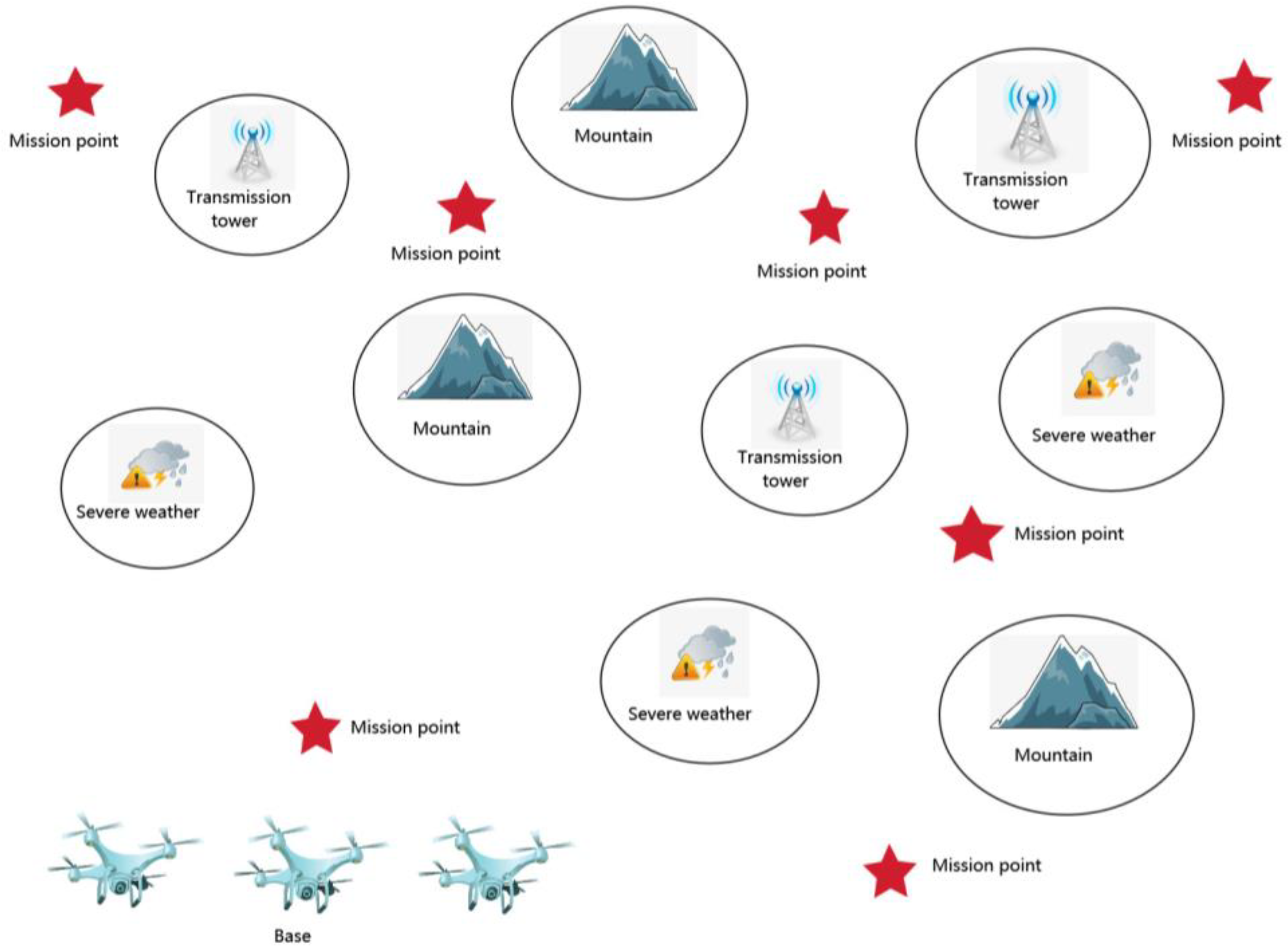
The method proposed in this paper is utilized to deploy multiple drones that originate from a base and perform disaster rescue missions at different target locations within the disaster area. The primary aim of these missions is to efficiently distribute vital supplies to the disaster-stricken region. Figure 1 shows a sketch of multi-drone disaster relief. Multiple mission points are situated in different locations within the disaster area, each requiring a specific quantity of rescue materials. Commencing from a designated starting point, multiple drones initiate the mission, transporting the materials to each mission point in the assigned order, and subsequently returning. The flight of the drone is affected by many factors, such as the mountains, transmitting towers, and severe weather. The mountain may affect the flight safety of drones. The transmitting tower may affect the communication system of the drone. Moreover, the severe weather may change the original flight path of the drone. In addition, flight distance and load will also affect the assignment of the entire mission.
In the aforementioned application scenario, multiple drones traverse N mission nodes in a specific sequence, starting from the base. Once the mission is accomplished, all drones return to the base. Assuming that N mission points are {x1, x2, …, xN}, the number of drones is M. Since the drone needs to return to the base after the mission is completed, we need to copy the base node as an M virtual base node. This enables the decomposition of the multi-path generation problem into one-way travel for a group of drones. This approach ensures that the flight path from the first drone to the last drone is connected from beginning to end, forming a single loop, as shown in Figure 2. Among them, O is the base node, and O1, O2, and O3 are the virtual base nodes.
If the mission of drone u includes the flight track from the mission point xi to the mission point xj, the decision variable is defined as = 1, otherwise = 0. The total flight distance of multiple drones is expressed as Equation (1). Equations (2) and (3) ensure that each mission point is visited only once during a mission cycle. Equations (4) and (5) specify that each drone can only take off and land at the base. Formula (6) ensures that the total flight displacement of each drone does not exceed its maximum flight displacement constraint. Equation (7) means that the load of each drone does not exceed its maximum load constraint.
where sij is the displacement between any pairs of target points (xi, xj); (Xi, Yi, Zi) and (Xj, Yj, Zj) are the 3D coordinates of mission points xi and xj, respectively; smax means the maximum displacement of drone driving; qi represents the material demand of mission point xi; and qmax means the maximum load of the drone.
3. Environment Modeling and Optimization Method
3.1. Proposed Flowchart
For multi-drone disaster rescue, it is crucial to design the mission sequence required by multiple drones for the whole rescue mission—that is, to plan the optimal mission assignment. In addition, to ensure a safe and effective drone flight, it is necessary to consider various threat sources when planning the drone’s flight path. Figure 3 shows the main process of multi-drone disaster rescue. First, before the mission planning of drones, it is essential to model the drone disaster relief environment. Then, a cost–revenue function is proposed based on drone performance and rescue scenarios. Finally, the AGA is used to realize the optimal mission assignment of multi-drones, and the SCPSO is employed for planning the optimal flight path between adjacent target points.
3.2. Construction of Original Digital Terrain
In the mission area, the safety constraints of the terrain should be considered while carrying out the material allocation. The original digital terrain refers to the basic surface appearance and terrain height in the 3D environment. Therefore, before carrying out multi-drone mission planning in a complex 3D disaster rescue environment, the original digital terrain must be constructed first. Without loss of generality, one of the reference models of the original digital terrain can be computed by the method in Formula (10). Other 3D terrains can also be obtained by satellite surveying and mapping.
where (x, y) is the two-dimensional coordinate of the horizontal projection plane; z1(x, y) represents the height information corresponding to the horizontal projection plane coordinates; a, b, c, d, e, and f mean the undetermined terrain coefficients. These coefficients control the amplitude of the ups and downs of the map and can simulate the actual terrain of various complex landforms. Currently, our hypothetical disaster rescue mission is conducted in the mountainous region of southwestern China, which is characterized by a complex climate and an extensive seismic belt, making it prone to natural disasters such as landslides and earthquakes. To describe the terrain of southwest China, we employ the subjective evaluation method for continuous parameter adjustments. Ultimately, the original terrain coefficients are set as a = 1.5 π, b = 5, c = 3, d = 5, e = 3, and f = 10, aiming to simulate the authentic topography of the region. Figure 4 is the corresponding simulated digital terrain.
3.3. The Modeling Method of Threat Source
It is assumed that there are three external threat sources for drone flight in our system: the mountains, transmission towers, and severe weather.
3.3.1. The Mountain Threat Source
The flight safety of the drone will be affected by the mountains. If the flight trajectory of the drone is not properly controlled, it may collide with the mountains and cause a crash. Therefore, it is important to plan the optimal scheme and path so that the drone can safely pass through the mountain area. The expression of the mountain mathematical model in this paper is shown in Equation (11). Additionally, a bi-Gaussian mixture model (bi-GMM) [43] (see Equations (12) and (13)) is used as the cost function of the mountain threat sources. This is due to its capacity to offer a smooth and continuous approximation of their shapes, rendering it better suited for real-world terrain in contrast to the traditional cone model that simulates mountain distribution.
where z1(x, y) means the peak elevation corresponding to point (x, y); n1 is the number of mountain threat sources; i is the ith mission point; N_m means the N_mth mountain threat source; hN_m is the height of the N_mth mountain threat source; (xO,N_m, yO,N_m) represents the central coordinate of the N_mth mountain threat source; xsl,N_m and ysl,N_m mean the slope parameters of the N_mth mountain threat source along the X-axis and Y-axis, respectively. Greater values of xsl,N_m and ysl,N_m indicate a flatter profile for the corresponding mountain threat source, while smaller values indicate a steeper profile. By manipulating the parameters hN_m, xsl,N_m, and ysl,N_m, it is possible to simulate mountain threat sources with varying heights and contours. The symbol fm(Xi, Yi) represents the probability density function of the bi-GMM model; (Xi, Yi) is the horizontal projection coordinate of the ith mission point; Cm is the cost function of the mountain threat source; N is the number of mission points; and k1 is the corresponding weight coefficient.
Finally, Equation (14) merges the mountain threat source with the original digital terrain to form a 3D environment-equivalent digital terrain, as shown in Figure 5.
where z(x, y) is the terrain height corresponding to the point (x, y); max means the function of the maximum value.
3.3.2. The Transmission Tower Threat Source
The electromagnetic interference emitted by the transmission tower can disrupt the communication and navigation systems of drones [44], potentially leading to the failure of accurate mission execution. Therefore, the position and influence range of the transmission tower needs to be considered when the drone is flying so as to reduce the risk of flight. The electromagnetic interference emitted by the tower can be regarded as the diffusion of a spherical model into space. In addition, the emitted electromagnetic interference should not have a specific limit, beyond which the risk of damage is zero. Therefore, a probability density model of the transmission tower threat source is proposed in this paper, as shown in Equations (15)–(17).
where ft(, ) represents the probability density model of the signal transmission tower threat source; N_t means the N_tth transmission tower threat source; i is the ith mission point; is the distance from the ith mission point to the threat source center of the N_tth transmitting tower; is the minimum safe distance of the N_tth transmission tower; σi,N_t means the control parameter of the probability density model of the transmitting tower; Li represents the distance from the current mission point to the ith mission point; Ct is the transmission tower threat source cost function; N is the number of mission points; n2 is the number of transmission tower threat sources; and k2 is the corresponding weight coefficient.
3.3.3. The Severe Weather Threat Source
Usually, when the drone is performing its mission, it may encounter local severe weather (such as storms, heavy rain, lightning, etc.). If the drone is compelled to operate in that environment, it may damage the motor or sensor of the drone or even crash. Therefore, drones need to change lanes to avoid severe weather. In this paper, severe weather events such as storms, rainstorms, and lightning are abstracted and simplified into cylindrical threat areas. A probability density model of the source of the threat of severe weather is shown in Equations (18) and (19).
where fw(, , ) means the probability density model of the threat source of severe weather; N_w is the N_wth severe weather threat source; i is the ith mission point; symbol means the risk coefficient of the N_wth severe weather; represents the distance from the ith mission point to the center of the N_wth severe weather threat source; is the minimum safe distance of the N_wth severe weather threat source; is the maximum impact range of the N_wth severe weather threat source; Cw means the cost function of the severe weather threat source; N is the number of mission points; n3 is the number of severe weather threat sources; and k3 is the corresponding weight coefficient.
3.4. The Cost–Revenue Function
In this paper, a cost–benefit function for multi-drone mission assignments is designed. When constructing the cost function, the influence of threat sources is considered, and the calculation methods are given in Equations (13), (17) and (19). The drone’s flight distance and flight elevation are also considered. Equations (20) and (21) give their calculation methods. Equation (22) represents the total cost function. The revenue function is expressed as the revenue from completing a mission. The greater the demand for materials at the mission point, the higher the revenue. Therefore, the revenue function can be expressed by Equation (23). Finally, the total cost–revenue function is expressed as Equation (24).
where Cdistance is the distance cost; k4 is the weight; Chigh is the elevation cost; k5 is the weight; the symbol means the quality of the drone u flying from the ith mission point to the jth mission point; hij represents the height difference between the ith mission point and the jth mission point; Ctotal means the total cost; Rtotal is the total revenue; kr is a weight, which is set to kr = 2 in this paper; qi means the material demand of the ith mission point; T represents a cost–revenue function; and ω1 and ω2 are weights, which are set to ω1 = 1 and ω2 = 1 in this paper.
3.5. Mission Planning Algorithms: AGA and SCPSO
An AGA method is designed for a multi-drone mission assignment, and a SCPSO algorithm is designed for 3D path planning.
3.5.1. The Mission Assignment of Multi-Drone Based on AGA
GA is a computational model that simulates the biological evolution processes of natural selection and genetics. In GA, each problem solution is represented as a set of chromosomes. Through selection, crossover, and mutation operations in each generation, GA gradually improves the quality of its solutions. The following are the calculation steps of the AGA algorithm.
- The population initialization
The initial solution to the mission assignment is generated by random numbers. Let us define the population size NAGA, the maximum iteration time TAGA, the maximum crossover rate PC,max, the minimum crossover rate PC,min, the maximum mutation rate PM,max, and the minimum mutation rate PM,min.
The initial chromosome is a Hamilton cycle [45]. In order to accelerate the convergence speed of the algorithm and obtain a better initial solution for each generation, the improved circle algorithm is used in AGA. That is, to judge whether two groups of adjacent gene points vp−1vp(p = 2, …, N − 2) and vrvr+1(r = p + 1, …, N − 1) in the chromosome meet the Equation (25). If it is satisfied, then vp and vr are arranged in the reverse order; otherwise, the next judgment is made until all gene points are traversed.
where dch means the distance between two gene points (mission points); vp is the pth gene point; and vr is the rth gene point.
- 2.
- The calculation of chromosome fitness
The chromosome fitness is the mission assignment fitness function in this paper, and its calculation is shown in Equation (26).
where represents the fitness function of the chrth chromosome in the tAGAth generation; T is defined in Equation (24).
- 3.
- The evolution of AGA
This step implements three operations: selection, crossover, and mutation. First, in the selection stage, the better the fitness, the greater the probability of producing excellent individuals. The method of roulette to choose (see Equation (27)) is used in this paper. Second, the two-point crossover is used in the cross-point phase; that is, two crossover points are randomly set for the chromosome, and then the chromosome gene sequence is cross-changed. Finally, the mutation phase is realized by randomly exchanging two genes in an individual.
where PS,tAGA,chr means the selection rate for the chrth chromosome of the tAGAth generation.
Without losing generality, we take seven gene points as an example. Figure 6 displays an example of AGA evolution. In Figure 6, two parent chromosomes are {7, 5, 3, 6, 2, 1, 4} and {4, 3, 1, 5, 2, 7, 6}, respectively, where the number represents the mission point. These chromosomes produce new fetus {7, 3, 1, 5, 6, 2, 4} through the two-point crossover. Finally, two gene points are randomly switched to obtain child {7, 6, 1, 5, 3, 2, 4}.
In order to improve the convergence speed and optimization effect of the algorithm, some computational strategies are designed in this paper. The crossover rate and mutation rate of AGA do not use setting values but are adaptively selected according to fitness changes, as shown in Equations (28) and (29).
where PC,tAGA,chr means the crossover rate of the chrth chromosome in the tAGAth generation; PM,tAGA,chr represents the mutation rate of the chrth chromosome in the tAGAth generation; kAGA1, kAGA2, kAGA3; and kAGA4 are the control coefficients, which are set to kAGA1 = 1, kAGA2 = 1.05, kAGA3 = 1, and kAGA4 = 1.25 in this paper. PC,max and PM,max represent the maximum values of crossover rate and mutation rate; PC,min and PM,min represent the minimum values of crossover rate and mutation rate; means the individual with the largest fitness in the tAGAth generation; represents the bigger fitness in the two chromosomes to be crossed in the tAGAth generation and is the average fitness of all chromosomes in the tAGAth generation.
In order to prevent the degradation of the genetic algorithm, the elite retention method for each iteration is adopted in this paper. That is, we retain the optimal individual of the generation for the next generation, do not participate in the evolution process, and compare it with the optimal individual of the next generation. If it is better than the next generation of optimal individuals, the algorithm continues to retain them; otherwise, the next-generation optimal individual is retained as an elite.
3.5.2. The Path Planning between Mission Points Based on SCPSO
PSO is derived from the study of bird predation behavior. The basic idea of the algorithm is to initialize a set of particles within the solution space that are explored in the search space. The characteristics of particles are expressed by velocity, position, and fitness. The velocity of each particle represents the moving direction of the particle; the position indicates the candidate solution of the optimization problem; and the fitness represents the quality of a solution. Each particle continuously adjusts its position through individual experience and group collaboration to find the optimal solution. In the path planning problem of this paper, each particle represents the coordinate of the path-control point. The following are the calculation steps of the SCPSO algorithm.
- The population initialization
In this step, the number of particles NSC, the number of path-control points NC, and the maximum number of iterations TSC are defined. The initial particle position (initial solution) is randomly generated in space.
- 2.
- The fitness function calculation
SCPSO calculates the fitness function of each particle at each iteration. The fitness function of path planning in this paper is expressed as the total distance of drone flight, as shown in Equations (30) and (31).
where represents the fitness function of the parth particle in the tSCth generation; PT is a penalty factor; lij,tSC,par means the length of the three-dimensional path planned by the parth particle of the tSCth generation of SCPSO between the ith mission point and the jth mission point; np is the number of path points of the three-dimensional path curve generated by the path-control point NC; means the sth path point of the three-dimensional path planned by the parth particle of the tSCth generation of SCPSO between the ith mission point and the jth mission point.
- 3.
- The iteration of SCPSO
Particle velocity is affected by inertia, individual optimal values, and global optimal values. Each particle adjusts the speed according to the current position, individual optimal value, and global optimal value, and then updates its position. The SCPSO algorithm proposed in this paper uses the properties of sine and cosine functions to improve the optimization ability of the algorithm by adaptively changing the amplitude of sine and cosine functions. In addition, in order to further balance the global exploration and local development capabilities of the algorithm, the inertia coefficient and acceleration coefficient of linear weights are also designed. Equations (32)–(37) show the speed and position update methods of the SCPSO algorithm.
where is the velocity of the parth particle of the tSCth generation on the dimth dimension; w represents the inertia weight coefficient; c1 means the individual acceleration coefficient, which is adaptively adjusted by Equations (35) and (36), respectively; rand() is the random number of [0, 1]; pbest,par,dim means the optimal position of the parth particle on the dimth dimension; represents the position of the parth particle of the tSCth generation on the dimth dimension; xsc means the sine and cosine components; R1 is the control parameter, which mainly controls the amplitude of the sine and cosine functions and adjusts adaptively through Equation (37); R2 and R3 are random numbers obeying a uniform distribution, which are set to R2 ∈ [0, 0.5π] and R3 ∈ [0, 1] in this paper; gbest,dim is the global optimal position on the dimth dimension; wmax and wmin are the maximum and minimum values of inertia weight; c1max and c1min are the maximum and minimum values of individual acceleration coefficient; and R1max and R1min are the maximum and minimum values of sine and cosine amplitude.
Finally, the individual optimal value and the global optimal value are updated according to the calculation results of SCPSO, and then the algorithm enters the next iteration.
4. Results and Discussions
Based on the above model research and algorithm designs, Python programming is used for simulation experiments on our PC (Intel(R) Core(TM) i7-10700K CPU @ 3.80 GHz, 32 GB RAM, NVIDIA GeForce RTX 3090). For the purpose of proving the effectiveness of the presented system and method, first the GA and the AGA are used to evaluate the mission assignment. Then, the evaluation experiments of three-dimensional path planning are carried out, in which PSO and SCPSO are compared. Third, the simulation experiment of a multi-drone disaster rescue system is carried out by combining mission assignment and path planning.
4.1. Comparison of GA and AGA
In this section, GA and AGA algorithms are compared. Mission points are used for gene coding on chromosomes. The initial population size NAGA of the algorithm is 200, the maximum crossover rate PC,max, and minimum mutation rate PC,min are 0.8 and 0.4, and the maximum crossover rate PM,max, and minimum mutation rate PM,min are 0.01 and 0.001. The experiment of multi-drone mission assignment is carried out in a 100 × 100 × 100 area. The drone base station coordinate is (2, 35, 1). Table 1 shows the parameters of each threat source. The experiment of three drones performing 10 mission points is evaluated and tested. The minimum fitness function and the mean fitness function of each generation with the maximum iteration time TAGA of 100, 200, and 300 are studied by performing 50 mission assignment experiments. Mission execution order, fitness function, and program running time are the main indexes of the mission assignment evaluation experiment. The fitness function is defined in Equation (24), where it is evident that a lower fitness function value indicates a better calculation outcome for the algorithm.
The maximum displacement of the drone is 300, the body weight is 1, and the maximum load is 4. Mission point coordinates and material requirements are shown in Table 2. Table 3 presents the comparison results of performance evaluation indexes between GA and AGA. The results indicate that the optimal value (OV), the worst value (WV), and the mean value (MV) of AGA are lower than those of GA except for the running time. Additionally, the lower standard deviation value (SDV) proves that AGA can obtain the optimal assignment stably. Figure 7 shows the statistical results of the minimum fitness per generation and the mean fitness per generation of GA and AGA with 100, 200, and 300 iterations, respectively. It can be seen from Figure 7 that the convergence speed and optimal value of AGA are much better than those of GA. Table 4 gives out the optimal mission execution order comparison result: when the iteration time is small, there are significant differences in the optimal allocation results between GA and AGA. However, when the iteration time is large, the optimal allocation results of GA and AGA become similar. AGA can achieve better results with fewer iterations.
4.2. The Evaluation Experiment of SCPSO
In this section, the evaluation experiment of the 3D path planning algorithm is carried out, and the PSO and SCPSO algorithms are compared. The initial population size (NSC) of the algorithm is 50. The number of path-control points (NC) is 5. The maximum inertia weights wmax and minimum inertia weights wmin are 0.9 and 0.4, respectively. The maximum individual acceleration coefficients c1max and minimum individual acceleration coefficients c1min are 2.5 and 1, respectively. Additionally, the maximum sine and cosine amplitudes R1max and minimum sine and cosine amplitudes R1min are 2.25 and 1. The experiment of multi-drone path planning is carried out in a 100 × 100 × 100 area, and the simulation time is 50. The starting point coordinate of the drone is (2, 35, 1), and the end point coordinate is (95, 80, 10). There are three threat sources: mountains, transmission towers, and severe weather. The parameters of each threat source are shown in Table 1. Table 5 presents the comparison results of performance evaluation indexes between PSO and SCPSO. Figure 8, Figure 9 and Figure 10 show the 3D path planning examples and statistical results of the minimum fitness and the mean fitness of each generation of PSO and SCPSO when the maximum iteration times TSC are 100, 200, and 300. The fitness function and program running time are the main results of this experiment. In 3D path planning, the fitness function refers to the distance of drone flight. Therefore, the smaller the fitness function value, the better the calculation effect of the algorithm. All the aforementioned evaluation experiment results demonstrate that SCPSO is capable of achieving a shorter flight path.
4.3. The Disaster Relief Simulation Experiment
This section conducts a multi-drone disaster rescue simulation evaluation experiment. Four algorithms, GA + PSO, GA + SCPSO, AGA + PSO, and AGA + SCPSO, are used for testing. The comprehensive evaluation of the multi-drone disaster rescue simulation evaluation experiment is carried out in a 100 × 100 × 100 area. The experiment of three drones performing 10 missions is evaluated and tested. The drone base station coordinate is (2, 35, 1), the number of path-control points NC is 2, the iteration times of GA and AGA are 300, the iteration times of PSO and SCPSO are 100, and the time of simulations is 20. The mission point, threat source, and other parameters of the algorithm are the same as those in Section 4.1 and Section 4.2. Table 6 shows the multi-drone optimal mission results of GA and AGA when the maximum iteration time is 300. Table 7 shows the evaluation results of four methods. It can be seen from Table 7 that the performance of AGA + SCPSO is the best, i.e., its fitness function is optimal and the path is the shortest. Figure 11 shows the visualization results of the drone disaster rescue experiment. It can be seen that the path planned by SCPSO is better, that is, its path is shorter and the route is smoother.
4.4. Discussions
After the disaster, due to the barrier of mountains and rivers, it is a challenging task for relief forces to reach the disaster area for the first time. Due to the urgency of disaster rescue, prompt execution of search and rescue operations within a short timeframe is often critical. The drone has the advantages of search and rescue [46], efficient monitoring [47], material distribution, and recovery of communication [48], which can be used for a fast disaster response [49]. Compared with a single drone, a multi-drone can undertake different rescue missions simultaneously and reduce rescue time. Therefore, it is necessary to study how to reasonably allocate different mission points for drones and plan their flight paths before implementing rescue. To this end, a multi-drone mission planning system and method that comprehensively consider factors such as flight distance, drone performance, threat source factors, and disaster site requirements are proposed in this paper. The research results can provide theoretical support for future disaster relief.
In this paper, three common threat sources in disaster rescue environments are modeled: mountains, transmission towers, and severe weather. Due to the characteristics of mountains, the mountain threat source is simplified by the bi-GMM. In future research, neural networks based on the truncated sign distance function (TSDF) can be used to model real mountain areas [50], making the model closer to real 3D mountain scenes. Although many anti-interference technologies have been developed to reduce the electromagnetic interference of drones [51], the signal is susceptible to weather, terrain, and other factors; so it is best to avoid entering the corresponding influence ranges. In the future, the interference of transmission towers and mining areas can also be studied. Modeling severe weather is a complex task due to its complexity and uncertainty and the vulnerability of drones to changes in airflow and pressure. In this paper, to enable fast computation, the range of influence of the severe weather threat source is abstracted using a cylinder. In the future, the difference in the response of drones’ own characteristics to weather phenomena and the temperature model [52] can be considered.
A cost–revenue function is formulated to facilitate multi-drone disaster relief mission allocation. The cost function represents the cost and risk of the multi-drone rescue process. In addition, due to the influence of weight on overcoming the work conducted by gravity, the order of mission execution is different, and the energy consumption of the drone is also varied. Therefore, the elevation cost is taken into account in the cost function. The revenue function represents the relief value of the task completed by the drone. The cost–revenue function represents the difference between the cost and revenue functions. Therefore, a smaller cost–revenue function indicates a better calculation effect for our model. In this study, the flight distance, flight height, threat source factors, drone performance constraints, and mission point revenue are all considered in the cost–revenue function. In the future, additional aspects can be taken into consideration when designing the cost–revenue function, such as the time required for a drone to perform different missions or the smoothness of the drone’s flight trajectory.
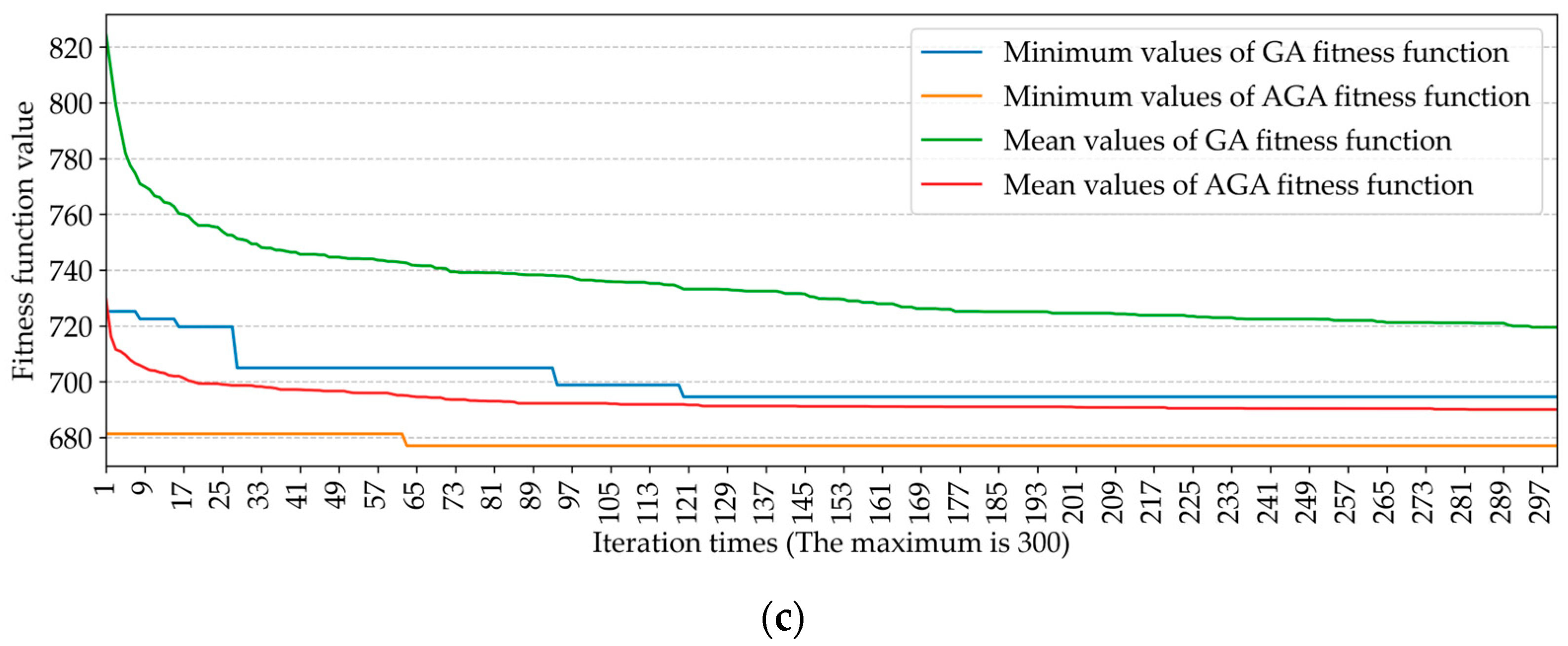
In this paper, AGA and SCPSO are used to assign missions and plan paths for drones, respectively. In order to further verify the effectiveness of AGA, we further supplement the comparative experiments of GA and AGA. In the 100 × 100 × 100 area, the experiment of 5 drones performing 20 missions is evaluated. The maximum displacement of the drone is 400, the body weight is 1, and the maximum load is 5. Mission point coordinates and material requirements are shown in Table 8. The remaining parameters are the same as those in Section 4.1. A total of 50 mission assignment experiments are performed. Table 9 presents a comparison of the performance evaluation indexes between GA and AGA for the corresponding disaster relief mission. It can be seen that in the case of increased task complexity, except for the program running time, the performance of AGA is significantly better than that of GA. Figure 12 shows the statistical results of the minimum fitness of each generation and the mean fitness of each generation for the corresponding GA and AGA when iteration times are 100, 200, and 300. It can be seen that the convergence speed, optimal value, and average value of AGA are much better than those of GA. Compared with the previous results (see Section 4.1), it can be seen that the higher the mission complexity, the better the performance of AGA. This means that the performance gap between AGA and GA is larger, and AGA is more suitable for mission assignments with high mission complexity. Table 10 presents the corresponding optimal mission execution orders for GA and AGA: as task complexity increases, the results show significant differences.
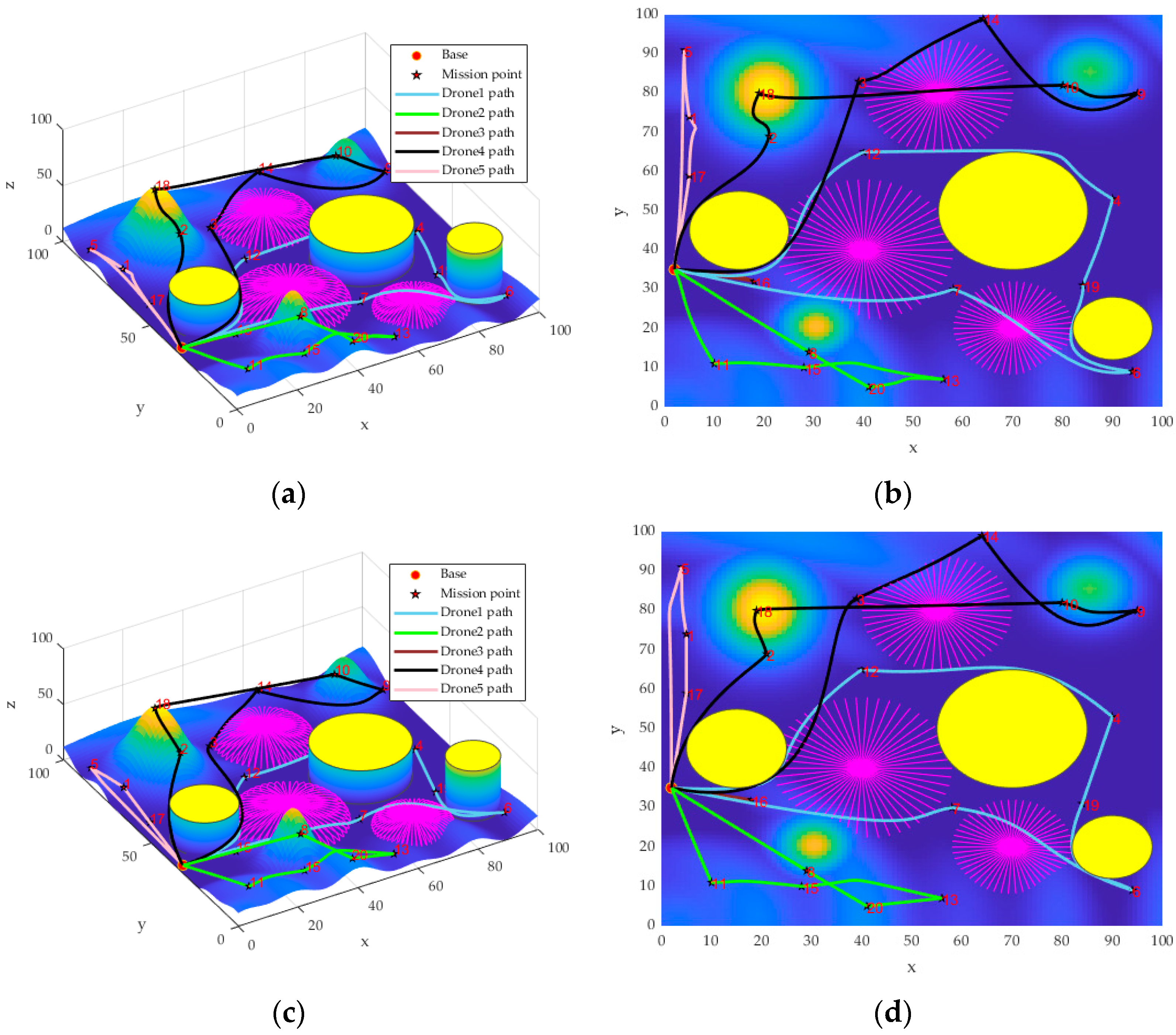
After repeated experiments, it can be found that GA is difficult to obtain optimal mission assignment with high complexity; differently, the AGA proposed in this paper can obtain optimal allocation only with fewer iterations. In order to further verify the effectiveness of SCPSO, we further supplement the comparative experiments of AGA + PSO and AGA + SCPSO under the same simulation experiment of 5 drones performing 20 mission points. The algorithm parameters are the same as those in Section 4.3. A total of 20 simulation experiments are performed. Table 11 shows the evaluation indexes of AGA + PSO and AGA + SCPSO. It can be seen that the performance of AGA + SCPSO is better in environments with higher mission complexity, i.e., the path is shorter and the route is smoother. Compared with the previous results in Section 4.3, it can be seen that SCPSO performs better when the mission complexity increases, and SCPSO is more suitable for path planning problems with high mission complexity. Figure 13 shows the visualization results of the corresponding drone disaster rescue experiment.
The effectiveness of the proposed model is demonstrated in this paper through a series of experiments. The fitness function and processing time are used in the experiment. When the number of missions is small, AGA generally reaches the optimal value within 10 generations, while GA needs hundreds of generations to reach the optimal value, and its optimal value is not as good as the optimal value of AGA. When the number of missions increases, AGA generally reaches the optimal value within 100 generations, while GA will use even 300 generations to reach the optimal value. Although AGA uses more computing resources and takes more computational time, it obviously takes less time if the time to reach the optimal value is discussed instead of the same number of iterations. For PSO and SCPSO, since SCPSO balances the ability of global and local optimizations, its convergence speed and optimal value are better than PSO. Clearly, all of the aforementioned experimental results demonstrate that our proposed method exhibits strong performance.
The method proposed in this paper has at least three advantages. First, the proposed system is designed to address the real-world scenarios of multi-drone disaster relief. The typical threat sources of disaster rescue scenarios, the requirements of disaster areas, and the performance of drones are considered when designing the cost–revenue function. This study can provide a basis for future drone disaster rescue. Second, for the problem of multi-drone disaster rescue, an optimization method with higher calculation accuracy is proposed, and this method is more suitable for optimization problems with high complexity. Third, the model has good scalability. Our model can simulate common disaster rescue scenarios and can be applied to various disaster relief environments with minimal modifications. Despite its advantages, our method also has limitations. For instance, our approach is specifically tailored for scenarios where complete environmental information is available. The presence of partially unknown information in the environment can potentially lead to mission planning failures. Moreover, an excessive amount of information regarding drones and mission points may have a detrimental impact on the real-time performance of the algorithm. These could be addressed in future work.
5. Conclusions
This paper realizes the problem of multi-drone mission planning in a complex 3D environment. The original digital terrain of drone flight and three common threat sources are constructed in this paper, including mountains, transmission towers, and severe weather. When constructing the cost–revenue function, factors such as the performance of the drone, the requirements of each mission point, the elevation cost, and the threat source are considered. AGA is designed to solve the problem of multi-drone mission assignments. The improved circle algorithm, adaptive crossover rate and mutation rate, and a strategy that uses both roulette and elite retention methods are used to improve the efficiency of our method. The experimental results demonstrate that AGA exhibits stronger optimization abilities than GA. SCPSO is designed to plan the optimal path between adjacent mission points. The inertia and acceleration coefficients of linear weights are designed to maintain an effective balance between global exploration and local development, further enhancing the performance of SCPSO. The experimental results show that the SCPSO algorithm can plan an effective and safe path for drones. This study can provide a basis for future disaster rescue decisions.
Author Contributions
Conceptualization, T.X., F.L., H.L. (Haoting Liu), J.G., H.L. (Hao Li), K.D. and Q.L.; data curation, T.X.; formal analysis, T.X., F.L., H.L. (Haoting Liu), H.L. (Hao Li), K.D. and Q.L.; funding acquisition, H.L. (Haoting Liu); investigation, T.X., F.L., J.G., H.L. (Hao Li), K.D. and Q.L.; methodology, T.X. and J.G.; project administration, F.L. and H.L. (Haoting Liu); resources, H.L. (Haoting Liu); software, T.X.; supervision, F.L. and H.L. (Haoting Liu); validation, T.X., F.L., H.L. (Haoting Liu), J.G., H.L. (Hao Li), K.D. and Q.L.; visualization, T.X.; writing—original draft, T.X.; writing—review and editing, T.X. and H.L. (Haoting Liu). All authors have read and agreed to the published version of the manuscript.
Funding
This work was funded by the National Natural Science Foundation of China under Grant 61975011, the Fund of Science and Technology on Near-Surface Detection Laboratory under Grant 6142414221403, the Fund of State Key Laboratory of Intense Pulsed Radiation Simulation and Effect under Grant SKLIPR2024, the Natural Science Foundation of Guangdong Province under Grant 2023A1515010275, and the Fundamental Research Fund for the China Central Universities of USTB under Grant FRF-BD-19-002A.
Data Availability Statement
The data used in this study are not public, but available upon request.
Conflicts of Interest
The authors declare no conflict of interest.
References
- Chen, M.; Wang, K.; Dong, X.; Li, H. Emergency rescue capability evaluation on urban fire stations in China. Process. Saf. Environ. 2020, 135, 59–69. [Google Scholar] [CrossRef]
- Díaz-Varela, R.A.; De la Rosa, R.; León, L.; Zarco-Tejada, P.J. High-resolution airborne UAV imagery to assess olive tree crown parameters using 3D photo reconstruction: Application in breeding trials. Remote Sens. 2015, 7, 4213–4232. [Google Scholar] [CrossRef] [Green Version]
- Boccardo, P.; Chiabrando, F.; Dutto, F.; Tonolo, F.G.; Lingua, A. UAV deployment exercise for mapping purposes: Evaluation of emergency response applications. Sensors 2015, 15, 15717–15737. [Google Scholar] [CrossRef] [PubMed] [Green Version]
- Ezequiel, C.A.F.; Cua, M.; Libatique, N.C.; Tangonan, G.L.; Alampay, R.; Labuguen, R.T.; Favila, C.M.; Honrado, J.L.E.; Caños, V.; Devaney, C.; et al. UAV aerial imaging applications for post-disaster assessment, environmental management and infrastructure development. In Proceedings of the 2014 International Conference on Unmanned Aircraft Systems, Orlando, FL, USA, 27–30 May 2014; pp. 274–283. [Google Scholar]
- Liu, H.; Yan, B.; Wang, W.; Li, X.; Guo, Z. Manhole cover detection from natural scene based on imaging environment perception. KSII Trans. Internet Inf. 2019, 13, 5095–5111. [Google Scholar]
- Whitehurst, D.; Joshi, K.; Kochersberger, K.; Weeks, J. Post-flood analysis for damage and restoration assessment using drone imagery. Remote Sens. 2022, 14, 4952. [Google Scholar] [CrossRef]
- Du, L.; Li, X.; Gan, Y.; Leng, K. Optimal model and algorithm of medical materials delivery drone routing problem under major public health emergencies. Sustainability 2022, 14, 4651. [Google Scholar] [CrossRef]
- Sun, Z.; Yen, G.G.; Wu, J.; Ren, H.; An, H.; Yang, J. Mission planning for energy-efficient passive UAV radar imaging system based on substage division collaborative search. IEEE Trans. Cybern. 2023, 53, 275–288. [Google Scholar] [CrossRef]
- Ramirez-Atencia, C.; Bello-Orgaz, G.; Camacho, D. Solving complex multi-UAV mission planning problems using multi-objective genetic algorithms. Soft Comput. 2017, 21, 4883–4900. [Google Scholar] [CrossRef]
- Mishra, B.; Garg, D.; Narang, P.; Mishra, V. Drone-surveillance for search and rescue in natural disaster. Comput. Commun. 2020, 156, 1–10. [Google Scholar] [CrossRef]
- Yamazaki, F.; Miyazaki, S.; Liu, W. 3D visualization of landslide affected area due to heavy rainfall in Japan from UAV flights and SfM. In Proceedings of the IEEE International Geoscience and Remote Sensing Symposium, Valencia, Spain, 22–27 July 2018; pp. 5685–5688. [Google Scholar]
- Fan, Q.; Wang, F.; Shen, X.; Luo, D. Path planning for a reconnaissance UAV uncertain environment. In Proceedings of the IEEE International Conference on Control and Automation, Kathmandu, Nepal, 1–3 June 2016; pp. 248–252. [Google Scholar]
- Yang, L.; Qi, J.; Xiao, J.; Yong, X. A literature review of UAV 3D path planning. In Proceedings of the 11th World Congress on Intelligent Control and Automation, Shenyang, China, 29 June–4 July 2014; pp. 2376–2381. [Google Scholar]
- Liu, H.; Ge, J.; Wang, Y.; Li, J.; Ding, K.; Zhang, Z.; Guo, Z.; Li, W.; Lan, J. Multi-UAV optimal mission assignment and path planning for disaster rescue using adaptive genetic algorithm and improved artificial bee colony method. Actuators 2022, 11, 4. [Google Scholar] [CrossRef]
- Debnath, S.K.; Omar, R.; Latip, N.B.A. A review on energy efficient path planning algorithms for unmanned air vehicles. In Proceedings of the Computational Science and Technology: 5th ICCST 2018, Kota Kinabalu, Malaysia, 29–30 August 2018; pp. 523–532. [Google Scholar]
- Fan, H.; Liu, F.; Xia, L. Cluster label aligning algorithm based on programming model. In Proceedings of the 24th Chinese Control and Decision Conference, Taiyuan, China, 23–25 May 2012; pp. 1768–1772. [Google Scholar]
- Ahner, D.; Parson, C. Weapon tradeoff analysis using dynamic programming for a dynamic weapon target assignment problem within a simulation. In Proceedings of the Winter Simulations Conference, Washington, DC, USA, 8–11 December 2013; pp. 2831–2841. [Google Scholar]
- Luo, W. An efficient sensor-mission assignment algorithm based on dynamic alliance and quantum genetic algorithm in wireless sensor networks. In Proceedings of the International Conference on Intelligent Computing and Integrated Systems, Guilin, China, 22–24 October 2010; pp. 854–857. [Google Scholar]
- Dumka, S.; Maheshwari, S.; Kala, R. Decentralized multi-robot mission planning using evolutionary computation. In Proceedings of the IEEE Congress on Evolutionary Computation, Rio de Janeiro, Brazil, 8–13 July 2018; pp. 1–8. [Google Scholar]
- Shahzad, A.; Ur-Rehman, R. An artificial intelligence based novel approach for real-time allocation of armament to hostile targets. In Proceedings of the 10th International Bhurban Conference on Applied Sciences & Technology, Islamabad, Pakistan, 15–19 January 2013; pp. 141–146. [Google Scholar]
- Huang, T.; Wang, Y.; Cao, X.; Xu, D. Multi-UAV mission planning method. In Proceedings of the 3rd International Conference on Unmanned Systems, Harbin, China, 27–28 November 2020; pp. 325–330. [Google Scholar]
- Pehlivanoglu, Y.V. A new vibrational genetic algorithm enhanced with a Voronoi diagram for path planning of autonomous UAV. Aerosp. Sci. Technol. 2012, 16, 47–55. [Google Scholar] [CrossRef]
- Yang, K.; Keat Gan, S.; Sukkarieh, S. A Gaussian process-based RRT planner for the exploration of an unknown and cluttered environment with a UAV. Adv. Robot. 2013, 27, 431–443. [Google Scholar] [CrossRef]
- Karaman, S.; Frazzoli, E. Incremental sampling-based algorithms for optimal motion planning. In Robotics: Science and Systems; MIT Press: Cambridge, MA, USA, 2011; Volume 6, pp. 267–274. [Google Scholar]
- Santiago, R.M.C.; De Ocampo, A.L.; Ubando, A.T.; Bandala, A.A.; Dadios, E.P. Path planning for mobile robots using genetic algorithm and probabilistic roadmap. In Proceedings of the IEEE 9th International Conference on Humanoid, Nanotechnology, Information Technology, Communication and Control, Environment and Management, Manila, Philippines, 1–3 December 2017; pp. 1–5. [Google Scholar]
- Medeiros, F.; Silva, J. A Dijkstra algorithm for fixed-wing UAV motion planning based on terrain elevation. In Proceedings of the 20th Brazilian Conference on Advances in Artificial Intelligence, São Bernardo do Campo, Brazil, 23–28 October 2010; pp. 213–222. [Google Scholar]
- Li, X.; Hu, X.; Wang, Z.; Du, Z. Path planning based on combination of improved A-star algorithm and DWA algorithm. In Proceedings of the 2nd International Conference on Artificial Intelligence and Advanced Manufacture, Manchester, UK, 15–17 October 2020; pp. 99–103. [Google Scholar]
- Wu, J.; Yi, J.; Gao, L.; Li, X. Cooperative path planning of multiple UAVs based on PH curves and harmony search algorithm. In Proceedings of the 2017 IEEE 21st International Conference on Computer Supported Cooperative Work in Design, Wellington, New Zealand, 26–28 April 2017; pp. 540–544. [Google Scholar]
- He, N.; Su, Y.; Guo, J.; Fan, X.; Liu, Z.; Wang, B. Dynamic path planning of mobile robot based on artificial potential field. In Proceedings of the International Conference on Intelligent Computing and Human-Computer Interaction, Sanya, China, 4–6 December 2020; pp. 259–264. [Google Scholar]
- Chen, Z.; Xu, B. AGV path planning based on improved artificial potential field method. In Proceedings of the IEEE International Conference on Power Electronics, Computer Applications, Shenyang, China, 22–24 January 2021; pp. 32–37. [Google Scholar]
- Cekmez, U.; Ozsiginan, M.; Sahingoz, O.K. A UAV path planning with parallel ACO algorithm on CUDA platform. In Proceedings of the International Conference on Unmanned Aircraft Systems, Orlando, FL, USA, 27–30 May 2014; pp. 347–354. [Google Scholar]
- Teng, H.; Ahmad, I.; Msm, A.; Chang, K. 3D optimal surveillance trajectory planning for multiple UAVs by using particle swarm optimization with surveillance area priority. IEEE Access 2020, 8, 86316–86327. [Google Scholar] [CrossRef]
- Cekmez, U.; Ozsiginan, M.; Sahingoz, O.K. Multi colony ant optimization for UAV path planning with obstacle avoidance. In Proceedings of the International Conference on Unmanned Aircraft Systems, Arlington, VA, USA, 7–10 June 2016; pp. 47–52. [Google Scholar]
- Daryanavard, H.; Harifi, A. UAV path planning for data gathering of IoT nodes: Ant colony or simulated annealing optimization. In Proceedings of the 2019 3rd International Conference on Internet of Things and Applications, Isfahan, Iran, 17–18 April 2019; pp. 1–4. [Google Scholar]
- Tian, J.; Shen, L.; Zheng, Y. Genetic algorithm based approach for Multi-UAV cooperative reconnaissance mission planning problem. In Proceedings of the International Syposium on Methodologies for Intelligent Systems, Bari, Italy, 27–29 September 2006; pp. 101–110. [Google Scholar]
- Zhao, J.; Zhao, J. Study on multi-UAV task clustering and task planning in cooperative reconnaissance. In Proceedings of the 6th IEEE International Conference on Intelligent Human-Machine Systems and Cybernetics, Hangzhou, China, 26–27 August 2014; Volume 2, pp. 392–395. [Google Scholar]
- Hu, X.; Ma, H.; Ye, Q.; Luo, H. Hierarchical method of task assignment for multiple cooperating UAV teams. J. Syst. Eng. Electron. 2015, 26, 1000–1009. [Google Scholar] [CrossRef]
- Wu, X.; Bai, W.; Xie, Y.; Sun, X.; Deng, C.; Cui, H. A hybrid algorithm of particle swarm optimization, metropolis criterion and RTS smoother for path planning of UAVs. Appl. Soft Comput. 2018, 73, 735–747. [Google Scholar] [CrossRef]
- Fu, Y.; Ding, M.; Zhou, C.; Hu, H. Route planning for unmanned aerial vehicle (UAV) on the sea using hybrid differential evolution and quantum-behaved particle swarm optimization. IEEE Trans. Syst. Man Cybern. Syst. 2013, 43, 1451–1465. [Google Scholar] [CrossRef]
- Tong, B.; Chen, L.; Duan, H. A path planning method for UAVs based on multi-objective pigeon-inspired optimization and differential evolution. Int. J. Bio-Inspired Comput. 2021, 17, 105–112. [Google Scholar] [CrossRef]
- Črepinšek, M.; Liu, S.-H.; Mernik, M. Exploration and exploitation in evolutionary algorithms: A survey. ACM Comput. Surv. 2013, 45, 1–33. [Google Scholar] [CrossRef]
- Pierpaoli, P.; Egerstedt, M.; Rahmani, A. Altering UAV flight path by threatening collision. In Proceedings of the Digital Avionics Systems Conference, Prague, Czech Republic, 13–17 September 2015; pp. 1–13. [Google Scholar]
- Xiong, T.; Zhang, L.; Yi, Z. Double Gaussian mixture model for image segmentation with spatial relationships. J. Vis. Commun. Image Represent. 2016, 34, 135–145. [Google Scholar] [CrossRef]
- Wang, Y.; Wang, H.; Xue, H.; Yang, C.; Yan, T. Research on the electromagnetic environment of 110kV six-circuit transmission line on the same tower. In Proceedings of the IEEE PES Innovative Smart Grid Technologies, Tianjin, China, 21–24 May 2012; pp. 1–5. [Google Scholar]
- Liu, L.; Luo, S.; Guo, F.; Tan, S. Multi-point shortest path planning based on an improved discrete bat algorithm. Appl. Soft Comput. 2020, 95, 106498. [Google Scholar] [CrossRef]
- Erdos, D.; Erdos, A.; Watkins, S.E. An experimental UAV system for search and rescue challenge. IEEE Aerosp. Electron. Syst. Mag. 2013, 28, 32–37. [Google Scholar]
- Yang, Z.; Yu, X.; Dedman, S.; Rosso, M.; Zhu, J.; Yang, J.; Xia, Y.; Tian, Y.; Zhang, G.; Wang, J. UAV remote sensing applications in marine monitoring: Knowledge visualization and review. Sci. Total Environ. 2022, 838, 155939. [Google Scholar] [CrossRef] [PubMed]
- Tuna, G.; Nefzi, B.; Conte, G. Unmanned aerial vehicle-aided communications system for disaster recovery. J. Netw. Comput. Appl. 2014, 41, 27–36. [Google Scholar]
- Khan, A.; Gupta, S.; Gupta, S.K. Emerging UAV technology for disaster detection, mitigation, response, and preparedness. J. Field Robot. 2022, 39, 905–955. [Google Scholar] [CrossRef]
- Qi, Z.; Zou, Z.; Chen, H.; Shi, Z. 3D reconstruction of remote sensing mountain areas with TSDF-based neural networks. Remote Sens. 2022, 14, 4333. [Google Scholar] [CrossRef]
- Zheng, T.; Sun, L.; Lou, T.; Guo, X.; Liu, Q. Determination method of safe flight area for UAV inspection for transmission line based on the electromagnetic field calculation. ShanDong Electr. Power 2018, 45, 27–30. [Google Scholar]
- Huang, L.; Peng, H.; Liu, L.; Li, C.; Kang, C.; Xie, S. An empirical atmospheric weighted mean temperature model considering the lapse rate function for China. Acta Geod. Cartogr. Sin. 2020, 49, 432–442. [Google Scholar]
Figure 1.
Sketch of multi-drone disaster relief.

Figure 2.
Sketch map of the multi-path problem into a single-path problem.

Figure 3.
Flow chart of the proposed system.

Figure 4.
Simulation result of the original digital terrain.

Figure 5.
Simulation result of the equivalent digital terrain.

Figure 6.
The example of AGA evolution.

Figure 7.
The fitness function evaluation results when the iteration times are 100, 200, and 300 (10 mission points). (a) The fitness function evaluation results (TAGA = 100). (b) The fitness function evaluation results (TAGA = 200). (c) The fitness function evaluation results (TAGA = 300).
Figure 7.
The fitness function evaluation results when the iteration times are 100, 200, and 300 (10 mission points). (a) The fitness function evaluation results (TAGA = 100). (b) The fitness function evaluation results (TAGA = 200). (c) The fitness function evaluation results (TAGA = 300).


Figure 8.
The 3D path planning examples and fitness function evaluation results of PSO and SCPSO (TSC = 100). (a) The 3D path planning diagram of PSO and SCPSO (TSC = 100). (b) The 3D path planning top view of PSO and SCPSO (TSC = 100). (c) The fitness function evaluation results of PSO and SCPSO (TSC = 100).

Figure 9.
The 3D path planning examples and fitness function evaluation results of PSO and SCPSO (TSC = 200). (a) The 3D path planning diagram of PSO and SCPSO (TSC = 200). (b) The 3D path planning top view of PSO and SCPSO (TSC = 200). (c) The fitness function evaluation results of PSO and SCPSO (TSC = 200).

Figure 10.
The 3D path planning examples and fitness function evaluation results of PSO and SCPSO (TSC = 300). (a) The 3D path planning diagram of PSO and SCPSO (TSC = 300). (b) The 3D path planning top view of PSO and SCPSO (TSC = 300). (c) The fitness function evaluation results of PSO and SCPSO (TSC = 300).


Figure 11.
Visualization results of a multi-drone disaster rescue simulation experiment under four methods (10 mission points). (a,b) visualization results of method GA + PSO; (c,d) visualization results of method GA + SCPSO; (e,f) visualization results of method AGA + PSO; (g,h) visualization results of method AGA + SCPSO.

Figure 12.
The fitness function evaluation results when the iteration times are 100, 200, and 300 (20 mission points). (a) The fitness function evaluation results (TAGA = 100). (b) The fitness function evaluation results (TAGA = 200). (c) The fitness function evaluation results (TAGA = 300).
Figure 12.
The fitness function evaluation results when the iteration times are 100, 200, and 300 (20 mission points). (a) The fitness function evaluation results (TAGA = 100). (b) The fitness function evaluation results (TAGA = 200). (c) The fitness function evaluation results (TAGA = 300).

Figure 13.
Visualization results of a multi-drone disaster rescue simulation experiment under different methods (20 mission points). (a,b) visualization results of method AGA + PSO; (c,d) visualization results of method AGA + SCPSO.
Figure 13.
Visualization results of a multi-drone disaster rescue simulation experiment under different methods (20 mission points). (a,b) visualization results of method AGA + PSO; (c,d) visualization results of method AGA + SCPSO.


Table 1.
Parameters of each threat source.
| No. | Center Coordinate, Slope, k1, and Height of Mountain Threat Source | Center Coordinate, k2, and Radius of Transmission Tower Threat Source | Center Coordinate, k3, , rN_w, and of Severe Weather Threat Source |
|---|---|---|---|
| 1 | (85, 85), (8, 8), 10, 40 | (40, 40), 20, 18 | (70, 50), 10, 0.6, 15, 25 |
| 2 | (20, 80), (10, 12), 10, 60 | (70, 20), 20, 12 | (15, 45), 10, 0.4, 10, 20 |
| 3 | (30, 20), (7, 7), 10, 50 | (55, 80), 20, 15 | (90, 20), 10, 0.2, 8, 18 |
Table 2.
Coordinates and requirements of 10 mission points.
| No. | Coordinate Mission Point | Requirement of Mission Point | No. | Coordinate Mission Point | Requirement of Mission Point |
|---|---|---|---|---|---|
| 1 | (5, 74, 10) | 0.9 | 6 | (94, 9, 7) | 0.7 |
| 2 | (21, 69, 35) | 0.7 | 7 | (58, 30, 1) | 0.9 |
| 3 | (39, 83, 4) | 1.3 | 8 | (29, 14, 37) | 0.5 |
| 4 | (90, 53, 1) | 0.8 | 9 | (95, 80, 10) | 1.1 |
| 5 | (4, 91, 3) | 0.4 | 10 | (80, 82, 34) | 0.6 |
Table 3.
Comparison of performance evaluation indexes between GA and AGA (10 mission points).
| Fitness Function (TAGA = 100) | ||||
|---|---|---|---|---|
| Method | OV | WV | MV | SDV |
| GA | 711.7506 | 763.4414 | 734.2795 | 13.9377 |
| AGA | 677.0911 | 703.6567 | 692.9914 | 7.1411 |
| Program running time (s) (TAGA = 100) | ||||
| Method | OV | WV | MV | SDV |
| GA | 10.8673 | 10.9425 | 10.8894 | 0.0155 |
| AGA | 10.9270 | 10.9460 | 10.9330 | 0.0038 |
| Fitness function (TAGA = 200) | ||||
| Method | OV | WV | MV | SDV |
| GA | 699.2446 | 752.1145 | 725.0800 | 11.8666 |
| AGA | 677.0911 | 703.0757 | 691.9700 | 7.1607 |
| Program running time (s) (TAGA = 200) | ||||
| Method | OV | WV | MV | SDV |
| GA | 21.6633 | 21.7874 | 21.7073 | 0.0225 |
| AGA | 21.7839 | 21.8891 | 21.8036 | 0.0147 |
| Fitness function (TAGA = 300) | ||||
| Method | OV | WV | MV | SDV |
| GA | 694.5612 | 745.4266 | 719.5153 | 13.8968 |
| AGA | 677.0911 | 698.4715 | 689.9750 | 6.1316 |
| Program running time (s) (TAGA = 300) | ||||
| Method | OV | WV | MV | SDV |
| GA | 32.4697 | 32.6227 | 32.5286 | 0.0322 |
| AGA | 32.6415 | 32.6807 | 32.6671 | 0.0090 |
Table 4.
Multi-drone optimal mission assignment of GA and AGA (10 mission points).
| Method | No. of Drone | TAGA = 100 | TAGA = 200 | TAGA = 300 |
|---|---|---|---|---|
| GA | 1 | 5, 1 | 5, 1 | 3, 5, 1 |
| 2 | 3, 4, 9, 10 | 3, 7, 6, 8 | 7, 6, 8 | |
| 3 | 7, 6, 8, 2 | 4, 9, 10, 2 | 2, 10, 9, 4 | |
| AGA | 1 | 3, 5, 1 | 3, 5, 1 | 3, 5, 1 |
| 2 | 7, 6, 8 | 7, 6, 8 | 7, 6, 8 | |
| 3 | 4, 9, 10, 2 | 4, 9, 10, 2 | 4, 9, 10, 2 |
Table 5.
Comparison of performance evaluation indexes between PSO and SCPSO.
| Fitness Function (TSC = 100) | ||||
|---|---|---|---|---|
| Method | OV | WV | MV | SDV |
| PSO | 117.6105 | 146.7281 | 129.5862 | 5.0713 |
| SCPSO | 108.7102 | 132.6111 | 115.7923 | 6.7508 |
| Program running time (s) (TSC = 100) | ||||
| Method | OV | WV | MV | SDV |
| PSO | 51.1639 | 64.1155 | 57.9294 | 3.2033 |
| SCPSO | 61.5123 | 66.3144 | 64.5302 | 1.2511 |
| Fitness function (TSC = 200) | ||||
| Method | OV | WV | MV | SDV |
| PSO | 116.1025 | 137.6843 | 125.6526 | 4.5177 |
| SCPSO | 108.6614 | 124.6490 | 114.0725 | 5.0003 |
| Program running time (s) (TSC = 200) | ||||
| Method | OV | WV | MV | SDV |
| PSO | 106.0202 | 124.9831 | 116.0116 | 5.0245 |
| SCPSO | 122.7706 | 134.3059 | 129.5099 | 2.1687 |
| Fitness function (TSC = 300) | ||||
| Method | OV | WV | MV | SDV |
| PSO | 114.6301 | 132.5005 | 122.0011 | 4.6042 |
| SCPSO | 108.6507 | 121.9915 | 113.1423 | 4.8832 |
| Program running time (s) (TSC = 300) | ||||
| Method | OV | WV | MV | SDV |
| PSO | 147.9369 | 186.1021 | 170.9336 | 8.1782 |
| SCPSO | 192.3480 | 204.1927 | 198.4601 | 2.7036 |
Table 6.
Multi-drone optimal mission results (the number of mission points is 10 and TAGA = 300).
| Method | No. of Drone | Optimal Mission Assignment Result |
|---|---|---|
| GA | 1 | 3, 5, 1 |
| 2 | 7, 6, 8 | |
| 3 | 2, 10, 9, 4 | |
| AGA | 1 | 3, 5, 1 |
| 2 | 7, 6, 8 | |
| 3 | 4, 9, 10, 2 |
Table 7.
The fitness function and path length statistics of four methods.
| Method | Optimal Fitness Function Value | Path Length | |||
|---|---|---|---|---|---|
| OV | WV | MV | SDV | ||
| GA + PSO | 694.5612 | 694.7434 | 739.5507 | 716.5673 | 11.2946 |
| GA + SCPSO | 694.5612 | 681.5401 | 737.6858 | 711.0448 | 14.5077 |
| AGA + PSO | 677.0911 | 691.8288 | 739.5353 | 716.0973 | 12.7313 |
| AGA + SCPSO | 677.0911 | 680.2483 | 737.5755 | 710.2630 | 14.7289 |
Table 8.
The coordinates and requirements of 20 mission points.
| No. | Coordinate Mission Point | Requirement of Mission Point | No. | Coordinate Mission Point | Requirement of Mission Point |
|---|---|---|---|---|---|
| 1 | (5, 74, 10) | 0.9 | 11 | (10, 11, 11) | 0.6 |
| 2 | (21, 69, 35) | 0.7 | 12 | (40, 65, 2) | 1.0 |
| 3 | (39, 83, 4) | 1.3 | 13 | (56, 7, 6) | 0.7 |
| 4 | (90, 53, 1) | 0.8 | 14 | (64, 99, 8) | 0.3 |
| 5 | (4, 91, 3) | 0.4 | 15 | (28, 10, 11) | 0.2 |
| 6 | (94, 9, 7) | 0.7 | 16 | (18, 32, 4) | 0.5 |
| 7 | (58, 30, 1) | 0.9 | 17 | (5, 59, 1) | 0.4 |
| 8 | (29, 14, 37) | 0.5 | 18 | (19, 80, 60) | 0.2 |
| 9 | (95, 80, 10) | 1.1 | 19 | (84, 31, 1) | 1.1 |
| 10 | (80, 82, 34) | 0.6 | 20 | (41, 5, 18) | 1.2 |
Table 9.
Comparison of performance evaluation indexes between GA and AGA (20 mission points).
| Fitness Function (TAGA = 100) | ||||
|---|---|---|---|---|
| Method | OV | WV | MV | SDV |
| GA | 1300.4399 | 1436.9930 | 1367.9740 | 31.1004 |
| AGA | 1005.1311 | 1063.0131 | 1038.3372 | 13.4497 |
| Program running time (s) (TAGA = 100) | ||||
| Method | OV | WV | MV | SDV |
| GA | 11.4349 | 11.4740 | 11.4482 | 0.0084 |
| AGA | 11.4968 | 11.5775 | 11.5298 | 0.0116 |
| Fitness function (TAGA = 200) | ||||
| Method | OV | WV | MV | SDV |
| GA | 1293.7675 | 1414.6581 | 1347.7407 | 29.4725 |
| AGA | 1001.0166 | 1056.1460 | 1035.4154 | 13.5783 |
| Program running time (s) (TAGA = 200) | ||||
| Method | OV | WV | MV | SDV |
| GA | 22.8013 | 22.8360 | 22.8165 | 0.0084 |
| AGA | 22.9302 | 23.0175 | 22.9803 | 0.0210 |
| Fitness function (TAGA = 300) | ||||
| Method | OV | WV | MV | SDV |
| GA | 1227.6617 | 1383.7537 | 1335.1681 | 29.8367 |
| AGA | 987.6911 | 1049.3092 | 1027.6919 | 14.2750 |
| Program running time (s) (TAGA = 300) | ||||
| Method | OV | WV | MV | SDV |
| GA | 34.1791 | 34.2579 | 34.1992 | 0.0152 |
| AGA | 34.3697 | 34.4926 | 34.4398 | 0.0322 |
Table 10.
Multi-drone optimal mission assignment of GA and AGA (20 mission points).
| Method | No. of Drone | TAGA = 100 | TAGA = 200 | TAGA = 300 |
|---|---|---|---|---|
| GA | 1 | 12, 2, 3, 14, 6, 13, 15 | 1, 12 | 7, 15, 11, 8 |
| 2 | 11, 17 | 17, 6, 19, 4, 7 | 13, 20 | |
| 3 | 19, 7, 4, 20, 8 | 10, 9, 14, 20, 11, 8, 15 | 17, 3, 12 | |
| 4 | 16, 18, 10, 9 | 16 | 16, 6, 4, 19, 10, 9 | |
| 5 | 5, 1 | 13, 5, 3, 18, 2 | 5, 1, 14, 18, 2 | |
| AGA | 1 | 11 | 9, 4, 19, 6, 7 | 7, 6, 19, 4, 12 |
| 2 | 15, 8, 20, 13, 6, 19, 7 | 11, 15, 20, 13, 8 | 8, 20, 13, 15, 11 | |
| 3 | 16 | 16 | 16 | |
| 4 | 4, 9, 10, 14, 18, 2 | 12, 3, 14, 10, 18, 2 | 3, 14, 9, 10, 18, 2 | |
| 5 | 17, 1, 5, 3, 12 | 17, 5, 1 | 5, 1, 17 |
Table 11.
The path length statistics of different methods.
| Path Length | ||||
|---|---|---|---|---|
| Method | OV | WV | MV | SDV |
| AGA + PSO | 936.6954 | 1016.0094 | 972.2957 | 19.4389 |
| AGA + SCPSO | 920.5319 | 1012.6603 | 967.2762 | 27.2980 |
Disclaimer/Publisher’s Note: The statements, opinions and data contained in all publications are solely those of the individual author(s) and contributor(s) and not of MDPI and/or the editor(s). MDPI and/or the editor(s) disclaim responsibility for any injury to people or property resulting from any ideas, methods, instructions or products referred to in the content. |
© 2023 by the authors. Licensee MDPI, Basel, Switzerland. This article is an open access article distributed under the terms and conditions of the Creative Commons Attribution (CC BY) license (https://creativecommons.org/licenses/by/4.0/).
Share and Cite
MDPI and ACS Style
Xiong, T.; Liu, F.; Liu, H.; Ge, J.; Li, H.; Ding, K.; Li, Q. Multi-Drone Optimal Mission Assignment and 3D Path Planning for Disaster Rescue. Drones 2023, 7, 394. https://doi.org/10.3390/drones7060394
AMA Style
Xiong T, Liu F, Liu H, Ge J, Li H, Ding K, Li Q. Multi-Drone Optimal Mission Assignment and 3D Path Planning for Disaster Rescue. Drones. 2023; 7(6):394. https://doi.org/10.3390/drones7060394
Chicago/Turabian StyleXiong, Tao, Fang Liu, Haoting Liu, Jianyue Ge, Hao Li, Kai Ding, and Qing Li. 2023. "Multi-Drone Optimal Mission Assignment and 3D Path Planning for Disaster Rescue" Drones 7, no. 6: 394. https://doi.org/10.3390/drones7060394