1. Introduction
In recent years there has been increasing interest in the use of drones, also known as unmanned aerial vehicles (UAVs), in urban areas for human, parcel, and food transportation in response to increasing urbanisation and climate change. The UN estimates that 68% of the world population will live in urban areas by 2050 [
1]. Transitioning part of ground transportation to the air can free up space on the surface. Furthermore, drone delivery has the potential to be more environmentally viable than current day ground-delivery [
2].
The European drone outlook study [
3] expects that there will be 400,000 drones in the air by 2050. Other estimates also point at densities previously unseen by traditional air traffic management [
4]. The U-space platform was established to support the creation of an infrastructure that provides a safe urban airspace in the European Union [
5].
Several projects developed comprehensive traffic management systems [
6,
7]. The main components of an air traffic management system are path planning, separation management, and airspace structure and rules. In highly-dense urban airspace these are interdependent and cannot be designed without considering the others. This work focuses specifically on the airspace structure and rules. An analogy from road traffic is useful to explain the difference between the structure and rules. Imagine a two-lane road (structure) in which each lane is reserved for a certain direction (rules). The rules provide guidance on how traffic is allowed to travel through the structure.
Urban airspace structures will be constrained by the existing urban environment [
8]. UAVs may have to operate above the road network in areas where buildings are tall. It may also be necessary to avoid flying over buildings for privacy reasons [
9]. Furthermore, the airspace is limited in height to reduce interference with general and civil aviation aircraft and because of limited energy capacity of drones so it is important to create rules that use the airspace effectively.
This work is interested in how different airspace structures and rules affect interactions between vehicles at a tactical level. As the density of the airspace increases, drones are more likely to encounter other drones. This can cause emergent behaviour that is detrimental to system safety. For this reason, the work uses separation minima as the measure of safety. This means that other factors of safety, such as meteorological impact or navigational performance are out of scope of this work. Moreover, the work also measures the route duration and route distances to provide an estimation of how the energy usage varies in the different airspace structures and rules.
Metropolis I [
10] investigated how different degrees of airspace structuring affect safety. The results showed that a layered concept was the safest. An important conclusion was that modifying the airspace structure and rules is an effective way to deal with detrimental emergent behaviour.
The work at hand aims to study emergent behaviour and evaluate the performance of a U-space system when applying strategic and tactical deconfliction methods. Various airspace structure and vertical altitude allocation rules, combined with established tactical deconfliction methods, are investigated under increasing level of traffic demand.
For this purpose, two sub-experiments are performed in order to isolate the effect of each on the performance of a U-space system. Sub-experiment 1 investigates different airspace structures in which layers are assigned a specific function (turning, cruising, deconflicting) [
11,
12]. Assigning layers for cruising will reduce the available airspace for other functions. Moreover, it is important to effectively utilise the available airspace because of the constrained nature of the airspace. Sub-experiment 2 investigates if it is beneficial to allocate drones to specific layers in the airspace or if it is better to allow the drones to redistribute based on the local situation.
Section 2 presents the general considerations for urban airspace design.
Section 3 presents the proposed airspace design configurations and the measures to analyse them.
Section 4 presents the experimental set up. The results of the experiments are presented in
Section 5. Finally, a discussion on the results and the conclusion are in
Section 6 and
Section 7, respectively.
2. Urban Airspace Design Considerations
This section first explains the main considerations for urban airspace design and then explains how airspace design can be evaluated. The main considerations for urban airspace design are:
Urban environment.
Airspace structure.
Airspace flight rules.
Other considerations.
2.1. Urban Environment
Flights operating in urban environments will need to regularly avoid static (i.e., buildings) and dynamic obstacles (i.e., other drones). The urban environment includes roads, geofences, and other infrastructure and these set the boundaries of where drones can operate. For example, drones may not be allowed to fly above parks or schools. The following section explains the different types of airspace environments (open and constrained) and how it relates to the urban environment. Furthermore, as the focus of this work is on constrained airspace, the effects of the city street network on constrained airspace design are described.
2.1.1. Types of Airspace
One study divided the urban airspace based on the height of the surrounding buildings [
13]. In areas with low-rise buildings, the airspace spanned from 0 to 500 feet (152.4 m) above the ground level. In areas with high-rises, the airspace began at the highest obstacle and ended 1000 feet (304.8 m) above it. Other work [
11,
12,
14] placed the airspace completely between buildings. In some cities (e.g., New York, Hong Kong) it may not be feasible for small UAVs to travel above the highest obstacle. Furthermore, for privacy considerations UAVs may avoid flying over buildings [
9,
15,
16].
It can be more helpful to define two types of airspace based on the degree of constraints, as shown in in [
7]. In
open airspace, drones can generally fly direct routes to their destination. Several workers have developed concepts operating in mostly open airspace [
6,
10,
17]. In
constrained airspace, drones were restricted to a predefined constrained network. The network may be constrained by the existing buildings (i.e., above roads) or by some virtual constraints. Several workers [
11,
12,
14,
18,
19,
20] developed concepts in which drones follow the network. It is important to note that the border between the two airspace types was not always clear. A mostly open airspace may have some geofenced areas and vice versa. However, this work separates them and specifically focuses on constrained airspace.
2.1.2. Effects of City-Layout on Constrained Airspace
Constrained airspace is highly dependent on the city layout [
8] when UAVs fly between the existing buildings. Cities like New York have highly orthogonal intersections [
21] which can simplify the urban airspace design parameters. For example, one airspace design may place UAVs on one of a set of four layers based on the cardinal directions of travel, north/east/south/west. This particular rule-set limits the chance of an encounter between UAVs travelling in different directions. Airspace designs in orthogonal networks were considered in [
11,
12,
18].
Many older cities are non-orthogonal, like in Europe [
21], which complicates the airspace design as there are now many different configurations of intersections. Applying the same design rule from the example in orthogonal networks is no longer trivial as a street that is currently facing the north direction may turn and face east in a non-orthogonal network. Furthermore, in non-orthogonal cities there can be a common leg being part of many shortest paths through the airspace. Drones sharing common legs create network hotspots if drones travel the shortest route to their destination. Airspace design in non-orthogonal networks were studied in [
7,
22]. This work focuses on constrained airspace in a non-orthogonal network.
2.2. Airspace Structures
Metropolis I project studied different urban airspace configurations above the buildings of Paris in open airspace [
10]. The study concluded that a layered airspace can help mitigate detrimental emergent behaviour at high traffic densities. Therefore, this work focuses on layered airspace. This section first explains the safety benefits of a layered airspace and then it shows how these are applied to constrained airspace.
2.2.1. Benefits of Layered Airspace Based on Track Angle
Figure 1 shows the layered open airspace from [
10]. Each layer only allows drones travelling in a specific heading range. This technique illustrates two interacting safety elements of a layered airspace, segmentation and alignment of the speed vector. Any finer airspace structure reduces the conflict rate by segmentation, which separates groups of drones. Using speed alignment lowers the relative velocity of drones in the same layer. An important takeaway is that adding constraints in an open airspace can have safety benefits [
23].
2.2.2. Adding Other Layer Types for Constrained Airspace
Layering has also been used in constrained airspace to achieve segmentation and alignment of drones [
11,
12,
14]. In [
11,
12] layers are assigned depending on the orientation of the street. The goal is to ensure that cruising drones from different streets are vertically segmented at the shared intersections. However, as drones cannot travel directly to their destination, they need to make turns in the network. In order to not overshoot, turning drones slow down to make the turn. However, decelerating for turns can create bottlenecks if there is a cruising drone behind the turning drone. One solution is to create a separate turn layer to which drones vertically manoeuvre before slowing down.
The three types of layers used in this study are: (1) Cruise, (2) turn, (3) buffer (
Figure 2). Cruise layers are where the drones spends the majority of the flight. Each cruise layer is assigned to a specific direction and it is assumed that drones cannot fly in parallel. Turn layers are used to transition from one cruise layer to another at an intersection. Finally, the buffer layers are an empty space created by the segmentation of the cruising layers, which also acts as a safety buffer against conflicts due to small vertical incursions.
There is a trade-off between the layer types because of the limited vertical space. Airspace designers cannot add an infinite amount of layers. If there is more cruising space provided it means that turning space is reduced and vice versa. In [
11,
12], turn layers were alternated with cruise layers to create a ‘1-to-1’ structure. Other structures, like in [
7], increased the amount of cruise layers by only giving one turn layer for every two cruise layers.
2.2.3. Applying Layers in a Constrained Airspace
In orthogonal networks the segmentation of layers can be achieved by considering the four possible directions of travel. Assuming that the network also aligns with the cardinal directions, the cruise directions are north, south, east and west. It is then possible to ensure that a north or south street never intersects at the same height as an east or west street.
It is more difficult to ensure segmentation in non-orthogonal networks than orthogonal ones because of the many different intersection configurations [
22]. An initially north-facing street may end up facing east at the next intersection. This makes it difficult to ensure that each intersection has segmented streets if the layer assignments are based on the cardinal directions. Moreover, the airspace quickly runs out if each unique street is assigned to a specific height. So using a cardinal assignment rule for segmentation means that there will be intersections where layers meet at the same height.
2.2.4. One-Way Networks and Layers
Studies have looked at comparing a one-way network versus a two-way network in orthogonal streets [
12]. In a one-way network, a street that is on the north–south line will have all cruise layers in that street facing one direction. In a two-way network the streets alternate in direction with increasing height. It was seen that a one-way network is safer as it reduces the chances of having head-on collisions because all UAVs in one street are aligned in their direction of travel. In an orthogonal network, the directional of parallel streets alternates to ensure that all intersections can be reached.
In a non-orthogonal network, it is not always possible to ensure that all intersections are connected with one-way networks. It is dependent on the network layout. As a result, a one-way network must be specifically designed to ensure that all intersections can be reached.
2.3. Vertical Allocation Rules in a Layered Airspace
In a layered airspace, the allocation of traffic to the vertical airspace also impacts the safety of the airspace. Ideally, each cruise layer of open or constrained airspace should maintain uniform distributions so one layer does not have denser traffic than another. Unfortunately, a uniform distribution is hard to achieve in urban air operations as some directions of travel may be preferred and it can depend on the time of day. This section outlines a safety concern from vertical manoeuvres and then explains vertical rule-sets for constrained airspace.
2.3.1. Vertical Manoeuvres
It is possible to ensure that in open airspace (
Figure 1) all layers are allocated a similar number of drones if there is a uniform distribution of origins and distributions. Moreover, there is no need to vertically transition between cruise layers except during take-off and landing. In [
24] it was seen that the drones performing vertical manoeuvres highly impacted the safety of the airspace. In a layered open airspace, vertical manoeuvres should be limited as much as possible since they create conflicts with drones in other layers that may have high relative velocities.
In the constrained airspace from
Figure 2 vertical manoeuvres are necessary for turns. Merging from the turn layer back to the cruise layer has a large impact on safety [
25]. However, it is not yet clear whether vertical manoeuvres between cruise layers in constrained airspace can also decrease the safety of the airspace.
2.3.2. Layer Allocation Rule-Sets in Constrained Airspace
In a one-way constrained layer airspace, such as in
Figure 2 the direction of travel does not change with height, thus the vertical allocation is not part in the structure. Therefore, explicit rules should be set for how the airspace is utilised to ensure an efficient spread of traffic.
Two different rule-set strategies can be described. The first are those that allocate a set of layers depending on some rules. Drones are allocated to a height and they must remain there until landing. An example rule allocation can use the distance of the mission. Short missions would be allocated to lower layers and long missions to higher layers. These strategies were used in [
11,
12] but were not a focus of the study.
Another strategy is one that does not try to pre-allocate layer sets and allows the drones to separate themselves based on the local density. An analogy is the ‘keep-right‘ car highway rule where cars must remain on the right unless they perform an overtake [
26]. In the Metropolis II project [
7], drones started their missions at the lowest layer set. However, if a drone approached a slower drone then it could vertically manoeuvre to a higher cruise layer, overtake, and then manoeuvre down again. This had the effect of ensuring that all drones remained in the available lower layers.
2.4. Other Considerations
The urban airspace cannot be designed without other components of a complete traffic management system, these are separation management and flight planning [
6]. These components are highly interdependent and should be designed in tandem. One reason is that the air densities are expected to be orders of magnitude higher than what is seen in conventional air traffic [
3,
4]. Another is that the expected missions (parcel and food delivery) are harder to plan in advance [
27]. For example, food delivery drones may be requested several minutes before the expected delivery rather than hours.
2.4.1. Separation Management
Separation management is the component that attempts to maintain safe separation of UAVs during their flight. Separation can be reached by de-conflicting paths prior to take-off (strategic) and by providing manoeuvres en-route that maintain separation minima (tactical). These separation minima and the prediction horizon have an impact on the design of the airspace structure. For example, in a layered airspace the separation minima influences the height of an airspace layer. There have been several U-Space projects that specifically focus on separation management [
28,
29].
2.4.2. Flight Planning
Flight planning is a main component of a safe traffic management system. Some work [
30] attempted to ensure that flight plans are deconflicted prior to take-off [
30]. In other work, each UAV planned their own shortest-distance route through the airspace [
12]. In a non-orthogonal constrained airspace, there are main streets which appear in many shortest routes which may create some local hotspots. Some airspace structures and allocation rules can cope better with these hotspots than others.
2.4.3. Out of Scope Considerations
This work is interested in how the interactions between vehicles affect the general safety and route duration and distance at increasing traffic demand. As a result, there are other important considerations for urban airspace design that are not considered for this work. These are drone hardware requirements, communication latency, emergency management, weather conditions. These can be found in several concepts of operations from [
5,
31].
3. Proposed Urban Airspace Concepts
Using the urban airspace design considerations, this section first proposes different airspace structures and allocation rule-sets. These also serve as independent variables in the experiments described further in this work. Following this, the dependent measures to evaluate the structures and rule-sets are presented. The airspace and rules are in the context of a non-orthogonal network under increasing imposed travel demand.
3.1. Layered Airspace Structures
This section illustrates two airspace structures that can be defined with the considerations from
Section 2.2. The function assignment of the layers is the main difference between the structures.
3.1.1. Baseline Constrained Airspace Structure
In the Baseline structure, the pattern seen in
Figure 2 where two orthogonal directions cross at different altitudes is repeated to reach the configuration seen in
Figure 3. This is the structure that was used in the Metropolis II study [
7]. The left and right stacks show the east/west and north/south layer configurations, respectively. Note that the grey layers in each structure correspond to altitudes where the other structure would have a cruising layer. For example, the lowest grey layer in the left image showing the east/west cruising layers corresponds to a blue cruising layer from the north/south assignment. The grey airspace is generally only used when making a vertical manoeuvre.
3.1.2. ‘1-to-1’ Constrained Airspace Structure
The ‘1-to-1’ structure alternates one cruise layer and one turn layer. It is a similar structure as that from [
11,
12]. The ‘1-to-1’ structure can be seen in
Figure 4. The alternation of layers reduces the amount of cruising space as compared to the Baseline structure. The ‘1-to-1’ structure has more layers for turning traffic. There are a total of 8 cruising layers in the ‘1-to-1’ structure versus 11 in the Baseline structure.
3.2. Vertical Allocation Rule-Sets in Layered Airspace Structures
This section illustrates four different vertical allocation rules. The Baseline concept attempts to give more freedom to how drones travel in an already constrained network. The three pre-allocated layer sets make drones more predictable because the heights at which drones may travel are predetermined.
3.2.1. Baseline Airspace Allocation
The Baseline rule-set aims to give freedom in how drones vertically separate themselves. This strategy is called the dynamic density redistribution algorithm which can be seen in Algorithm 1 [
7]. Essentially, the principle is the same as in the ’keep-right’ case for highways, the drones remain on the lowest cruise layer. However, if a faster drone approaches a slower drone in front, then it can perform a vertical manoeuvre to move up a layer, then overtake manoeuvre and then return to the lower layer. The conflict resolution (CR) algorithm can also call for vertical solutions if necessary. However, the extra freedom in vertical manoeuvres comes at the cost of increased airspace complexity.
Figure 5 illustrates the procedure for performing a vertical overtake. Drones A and B are both travelling in the lower cruise layer with a speed of 30 and 20 knots (15.4 m/s and 10.3 m/s), respectively. As drone A approaches drone B, it checks if the cruise layer above is empty. If there are no drones above then it can ascend.
Figure 6 illustrates the procedure of returning back to the lowest layer after an overtake. If there are no drones in the cruise layer below, then the drone can descend.
These proactive manoeuvres aim to reduce congestion at the local level. However, it is also important to note that not all transitions are proactive. Turn transitions are those that occur when a drone transitions to a turn layer from a cruise layer or vice versa. These are ’forced’ transitions and occur at all turns of the flight. The CR algorithm may also perform some ‘reactive‘ vertical transitions.
| Algorithm 1 Dynamic density redistribution algorithm. |
1: for each drone in constrained airspace do 2: if drone in conflict then: ▹ conflict resolution algorithm takes over |
3: return CR manoeuvre |
4: else: |
5: if drone in lowest cruise layer then: |
6: if no drone in front then: ▹ drone remains |
7: return Maintain altitude, continue cruising |
8: else: ▹ drone ascends |
9: return Drone received ascend command |
10: else: |
11: if no drone in cruise layer below then: ▹ drone descends |
12: return Drone receives descent command |
13: else if drone in front then: ▹ drone ascends |
14: return Drone receives ascent command |
15: else: ▹ drone remains in current layer: |
16: return Maintain altitude, continue cruising |
3.2.2. Other Allocation Methods
The pre-allocated rule-sets aim to distribute drones uniformly over the layers to create a ‘keep-lane‘ strategy.
Figure 7 shows five different layer set allocations stacked on top of each other. In the allocation concepts, drones transition to a pre-determined layer set and stay there throughout their route. Each layer set has one north/south cruise layer and one east/west cruise layer. Note that these sets do not use the highest layer as it does not have an accompanying red cruise layer. However, the effect is minimal when compared to the dynamic density redistribution algorithm because it ensures that the highest layer of the airspace is rarely used. The three different height allocations strategies are:
Density allocation: This allocation uses the current density in constrained airspace. When a drone enters the airspace it is allocated to the layer set with the least number of drones in it. If there are two or more sets with the same number of drones then it gets allocated to the lowest layer set.
Random allocation: Whenever a drone enters the airspace it is randomly allocated to a layer set. This method attempts to give a uniform distribution without the need for any knowledge of the current occupation levels of the layer sets.
Flight distance allocation: Drones are allocated to a layer set depending on the flight distance. Shorter flights are in lower layers and longer ones are higher. The distances per layer set are seen in
Table 1. They are based on one experimental scenario and attempt to set the same density at each layer set. So it is similar to using historical distance-distribution traffic data for the airspace rules.
3.3. Evaluating the Concepts
This section explains the dependent measures that are used to evaluate the different proposed structures and vertical allocation rule-sets. Four different categories of dependent measures are used, (1) achieved density, (2) vertical transitions, (3) airspace safety, and (4) route duration and distance.
3.3.1. Achieved Density
The safety of a layered airspace is directly related to the density of drones in that layer [
24]. The more drones there are the higher chance that they may encounter each other. With more interactions, drones may slow down as they must adjust their speed, like cars in busy highways.
In this study, the total airspace area is kept constant, therefore the concurrent number of drones in the air can be used as a way to measure resulting traffic density. Additionally, for the allocation rule-sets, it is also helpful to measure the concurrent number of drones in the airspace per layer set.
3.3.2. Vertical Transitions
The different allocation rule-sets affect how the drones vertically manoeuvre in the airspace. As it was seen in [
24], vertical transitions can destabilise layered open airspace as they increase the vehicle to vehicle interactions. Therefore, this work measures the average number of vertical transitions per flight when comparing rule-sets to analyse if this is indeed the case for constrained airspace.
There are different types of vertical transitions. These are (1) dynamic density redistribution transitions, (2) turning and (3) conflict resolution. It is also possible that a transition is interrupted due to an unforeseen conflict.
3.3.3. Safety
In the current work, safety is evaluated by counting conflicts and intrusions. Conflicts and intrusions are tactical dependent measures as they give an idea on the vehicle-to-vehicle interactions. These are safety dependent measures that have been used in previous research [
7,
10,
11,
12]. Those were inherited from traditional air traffic management (ATM) in which aircraft have a cylindrical protected zone, i.e., a horizontal circle with a vertical height. These make up the horizontal and vertical separation minima that is used in this work.
An intrusion occurs when the distance between two drones is less than the predefined separation minima. A conflict is a predicted intrusion. State-based conflict detection can be used for conflict counting. At each time step the current state of the drones is linearly extrapolated into the future with a certain look-ahead time. If an intrusion is expected to occur, then a conflict is counted. A drone may alter its current state to avoid the intrusion by performing conflict resolution. Performing conflict resolution manoeuvres may lead to longer missions.
Figure 8 illustrates the difference between a conflict and an intrusion in two dimensions. The left side illustrates a conflict between the ownship (black) and intruder (red). The horizontal minima is illustrated with a dotted black circle around the ownship. If both drones maintain their current state it is predicted that the intruder will enter the protected zone of the ownship within the lookahead time. The right image shows an intrusion. An intrusion occurs when the conflict is not solved and the intruder enters the dotted circle. Each drone performs conflict resolution manoeuvres to ensure that conflicts do not become intrusions. This work measures the average number of conflicts and intrusions per flight.
Since, the allocation rule-sets also study the vertical transition types it is useful to identify the average number of conflicts per flight attributed to a transition and the percentage of those in regards to the total conflicts per flight. Additionally, it is also possible to analyse the layer-types of two drones in an intrusion. If the drones are in the same layer, then it means that the intrusion was likely caused by a merging or in-trail conflict. Alternatively, if they are in different layers then the intrusion was caused by a vertical transition.
Defining the safety dependent measures in terms of conflicts and intrusions can provide some limitations. For example, the separation distances and look-ahead times will affect the observed number of conflicts and intrusions. As a result, the actual values of the separation distances and look-ahead times are not important for this work. The absolute number of conflicts and intrusions do not provide sufficient information to asses safety. A meaningful analysis can be made by making comparisons between the concepts and studying how that difference is affected by increasing traffic demand.
In the future, the separation standards of drones should consider several factors. These are communications, navigation and surveillance (CNS) factors which affect accuracy of position detection, and data transmission latencies [
31]. Moreover, the separation distance may be affected by the local weather conditions, size of the aircraft, type of mission, and ground risk [
13].
3.3.4. Route Duration and Distance
This work does not include an energy model to calculate the energy usage. Therefore, it is indirectly evaluated by looking at the average route duration and distance of flights. Due to the simplicity of the calculation, the absolute numbers are not important. Meaningful results are attained with relative comparisons. The route duration and distance dependent measures are shown as percentages of the Baseline concept. For example, the vertical distance percentage for a non-baseline concept is defined by the following equation:
The same can be achieved for 3D distance and route duration. For these dependent measures, the value is larger than 100% when drones tended to travel more distance or time when compared to the Baseline structure or allocation method.
4. Comparative Experiment
With the proposed concepts in
Section 3 this section first outlines experimental hypotheses. Then, it introduces the independent variables, dependent measures, and the simulation set up.
There are two sub-experiments. Sub-experiment 1 studies how varying layer function assignment of the airspace structure affects the overall system safety, and route distance, and route duration. Sub-experiment 2 studies how modifying the vertical allocation rule-sets affects the overall system safety, and route distance, and route duration.
4.1. Hypotheses
These airspace structures and vertical allocation rule-sets can compared against each other under increasing traffic demand.
4.1.1. Sub-Experiment 1
Hypothesis: Structures 1 (S1): In the lower traffic demands, safety differences are not expected. However, as the demand increases, Baseline structure is hypothesised to be safer than the ‘1-to-1’ structure because the ‘1-to-1’ contains less cruising layers. Having more cruising space will help drones in the Baseline deal with detrimental emergent behaviour at high demands. The lower amount of cruise layers in the ‘1-to-1’ structure will mean that there are more drones per cruise layer. Therefore, drones in the ‘1-to-1’ concept are more likely to encounter each other and cause higher number of conflicts and intrusions per flight.
Hypothesis: Structures 2 (S2): In the all traffic demands, drones in the Baseline structures are hypothesised to have shorter route distances because there is less space between cruise layers as compared to the ‘1-to-1’ structure. The less space between cruise layers would mean that drones travel less vertical distance when making a vertical manoeuvre.
As traffic demand increases, and the number of conflicts and intrusions increase (Hypothesis S1), drones in the ‘1-to-1’ concept will begin to have longer route durations for a longer time as they must slow down due to interactions with other drones.
4.1.2. Sub-Experiment 2
Hypothesis: Allocation 1 (A1): At all traffic demands, the Baseline is expected to have the highest amount of drones in the lowest layer set. The three allocation rules are hypothesised to spread traffic evenly across each layer set despite the different allocation method at all traffic demands.
Hypothesis: Allocation 2 (A2): Differences in safety are not expected in the lower traffic demands. At higher demands, the Baseline concept is hypothesised to be safer than the three allocated concepts because drones are able to vertically redistribute themselves based on the local traffic conditions. These proactive vertical transitions may lead to fewer conflicts and intrusions per flight.
Moreover, differences in safety between the three pre-allocated rule-sets should not be observed across traffic demands because they all attempt to spread traffic uniformly across the airspace.
Hypothesis: Allocation 3 (A3): At all traffic demands, drones in the the Baseline concept are hypothesised to travel longer distances and route durations than the other allocation rule-sets. Even though drones stay lower in the airspace, the increased vertical manoeuvres are expected to create longer travel times and distances.
Between the three pre-allocated concepts, the Flight Distance method is expected to have shorter distances and route durations because drones with the shortest paths will have shorter take-off distances.
4.2. Independent Variables
The two experiments presented in this work are structured around different sets of independent variables. Sub-experiment 1, which investigates the effects of airspace structure on the performance of the U-Space system, includes the following independent variables:
The second sub-experiment, which investigates the effects of the vertical allocation rule-set on the overall performance of the U-space system, includes the following independent variables:
It should be noted that Sub-experiment 1 uses the baseline allocation method described in
Section 3.2.1 throughout all the experiment conditions. Similarly, Sub-experiment 2 uses the baseline airspace structure throughout all the experiment conditions, described in
Section 3.1.1.
4.3. Dependent Measures
The following section presents a summary of the dependent measures (first introduced in
Section 3.3) used for each sub-experiment. Not all measures were deemed relevant for the first sub-experiment. Thus, the following set of dependent measures were used for Sub-experiment 1:
Number of drones concurrently in flight,
Conflicts per flight,
Intrusions per flight,
Vertical distance travelled as a percentage relative to the baseline condition of the sub-experiment, and
Route duration as a percentage relative to the baseline condition of the sub-experiment.
All the dependent measures used for Sub-experiment 1 are also relevant for Sub-experiment 2, and are thus also recorded. However, additional measures applicable to Sub-experiment 2 only were also recorded:
Number of drones concurrently in flight per layer set,
Number of vertical transitions per flight (includes total, dynamic density redistribution, turn, and interrupted transitions),
Percentage of conflicts attributed to a vertical transition,
Number of intrusions within each layer type per flight, and
The three-dimensional distance travelled as a percentage with respect to the baseline condition of the sub-experiment.
4.4. Simulation Set-Up
4.4.1. Imposed Traffic Demand
Each concept is tested under five imposed traffic demands with increasing number of flights, similar to [
7].
Table 2 shows the imposed concurrent average number of drones and the average instantaneous traffic density. The flight plans are created prior to the simulation. Take-offs are then scheduled so that the concurrent number of drones in the area remains approximately constant if all drones depart on time and travel with their average speed. For each imposed demand there are nine scenarios (or repetitions) with varying flight plans. Each scenario accommodates 1 h of spawning traffic.
4.4.2. Simulation Area
This work considers the airspace of Vienna as used in Metropolis II [
7]. The airspace is an 8 km radius circle, see
Figure 9. The area seen in the middle is constrained airspace, Drones must follow the existing road network in this area. The existing road network is sourced from OpenStreetMap [
32] using the OSMnx python library [
33]. Drones may travel directly to their destination in the part of the airspace that is open.
Although the simulation area also includes open airspace, the focus of the analysis is on constrained airspace.
Figure 10 shows the layer assignments of each street in constrained airspace. Red layers are generally in the north or south directions. Blue layers are generally in the east or west direction. Note that the constrained network is one-way so each street only allows one direction of travel.
4.4.3. Vertical Airspace and Layer Heights
The vertical airspace ranges from 0 to 500 feet (152.4 m) with each vertical layer measuring 30 feet (9.14 m) for a total of 16 layers. The first layer is centred at 30 feet above the ground. Note that this work does not suggest that vertical layers in urban airspace are mandated to be 30 feet. The real value will depend on safe separation specifications (
Section 3.3.3). The 30 feet is an arbitrary value to fit several layers inside the airspace. The absolute number of layers can be increased or decreased depending on the real specification.
4.4.4. Vertiports and Distribution Centres
Vertiports are spaced throughout the districts of Vienna. Each vertiport covers a maximum of 0.5 square km. The vertiports are uniformly distributed per district and the number of vertiports in a district depends on financial and population metrics [
7]. Additionally, there are 16 distribution centres placed around Vienna (see
Figure 1 of [
7]).
For this work, it is assumed that 40 percent of traffic originates from the distribution centres and goes to a vertiport. The other 60 percent of traffic starts and ends at a vertiport.
4.4.5. Missions
There are three different types of missions in the simulations: (A) Point-to-point, (B) distribution centre-to-point, (C) emergency. This was defined in order to differentiate between parcel deliveries, which typically originate in a distribution centre, and missions like food deliveries, which would be labelled as point-to-point. Emergency vehicles are a small percentage of the traffic and are allowed to violate the rules of the airspace to reach their destination.
Mission types (A) and (B) were also given a priority. Each of these drones were assigned to low, medium, or high priorities. Each priority accounted for about a third of the traffic. Drones with higher priority (e.g., medical deliveries) have more importance in the separation management decisions.
All missions start at ground level and then begin take-off. Drones take-off if there are no other drones near them. If the drone is not able to find space within 5 min of its scheduled departure then it takes-off. Note the the landing portion of the mission is removed and the drone disappears from the simulation once it is above the destination. The missions are designed to take an average of 15 min and is at least 1 km long.
4.4.6. Drone Models
For this experiment two drone types based on the DJI Matrice 600 Pro hexacopter drone model was used for the simulations. Their only difference is the average cruising speed (
Table 3).
4.4.7. Path Planning and Capacity Monitoring
The output of the flight planning module was a list of sequential waypoints to guide drones to their selected destination. Each mission created a flight plan through the airspace that did not violate the rules.
Flight planning was achieved via the D* Lite algorithm [
34]. The path planning graph was based on the street network, with the street sections acting as graph edges and the street intersections acting as graph nodes (
Figure 10). The path planning algorithm computed the most efficient path on the described path graph, minimising the duration of the path.
Two optimisation parameters were used to indirectly minimise the duration of the flight: (1) The length of the path, and (2) the number of turns. Each turn required additional time for slowing down to turn to ensure that they do not overshoot, therefore it was assumed that the duration of the path depended on the number of turns. Both the cost and heuristic functions, used by the D* Lite algorithm implemented for this system, implemented the two optimisations. The path’s length was divided by the nominal speed from
Table 3 to compute the duration of the path. Then, an additional cost due to turning of 1.83 s per turn was added to the cost and heuristic functions.
There is a central capacity monitoring module active for Sub-experiment 1. Capacity monitoring gathered position data from all drones and estimated the current image of the traffic density. The cost of traversing a street was updated, depending on the current traffic density, and sent to the drones for replanning. Note that the capacity monitoring was turned off in Sub-experiment 2 as it was not applicable because it acted on two dimensions and sub-experiment distributes traffic in three dimensions.
4.4.8. Conflict Detection and Resolution
The current work used conflicts and intrusions as safety measures. An intrusion occured when the distance between two drones was less than a predefined separation minima. In the current work, the horizontal distance was 32 m and the vertical was 7.62 m [
35] (Table 3.7.2.4-1). State-based conflict detection with a 10 s look-ahead time was used.
Drones may employ altitude and speed-based conflict resolution manoeuvres. Note that for the pre-allocation rule-sets, the vertical conflict resolution manoeuvres were not performed because of the rules of the airspace. The conflict resolution algorithm can be studied more in detail in [
7].
4.4.9. Turning in Constrained Airspace
Drones in constrained airspace performed turns to avoid collisions with buildings. However, drones must slow down from the cruising speeds in order to avoid overshooting the turn. In this work drones vertically transitioned from cruise layers to turn layers prior to turning. The drones then decelerated to make the turn. After making the turn, the drones accelerated and then merged back into the cruise layer. Note that the conflict resolution algorithm may interrupt the vertical transitions associated with turning.
4.4.10. Simulation Software
This work used the BlueSky air traffic simulator for the experiments [
36]. BlueSky can be extended via plugins and conditional commands in flight plans such that different airspace structure and rules can be compared against each other with similar conditions. This work also made use of the Metropolis II developments for BlueSky. These developments improved the capabilities of simulating traffic in urban environments.
5. Results
The following section shows the results of the two sub-experiments. Unless noted otherwise, the density plots show the number of drones in the vertical axis and the time in the horizontal. The vertical transition and safety plots have the corresponding measure on the vertical axis and the imposed traffic demand in the horizontal. The route duration and route distance plots are similar to the vertical transition and safety plots, with the difference being that the Baseline is seen as a horizontal line at 100%.
5.1. Sub-Experiment 1
Sub-experiment 1 compared the Baseline structure to the ‘1-to-1’ structure. The results are presented in the following section. Note that there were no observed differences in achieved density between structures.
5.1.1. Safety
Figure 11a,b show the number of conflicts and the intrusions per flight in constrained airspace, respectively, for the two structures. The Baseline structure had more conflicts than the ‘1-to-1’ structure at all imposed demands. In terms of intrusions, the two structures were similar at the lower imposed demands. However, the ‘1-to-1’ structure had more intrusions at the high and very high demand.
5.1.2. Route Duration and Distance
Figure 12 shows the percent of vertical distance travelled of the ‘1-to-1’ structure compared to the Baseline at all imposed demands. The drones in the ‘1-to-1’ structure travelled more vertical distance.
Figure 12 shows the percent of route duration with respect to the Baseline. It is clear that at most imposed demands the difference between the structures is negligible. At the very high demand, drones in the ‘1-to-1’ structure spend more time in the air than drones in the Baseline.
5.2. Sub-Experiment 2
Sub-experiment 2 compares the density redistribution algorithm to three other pre-allocation methods.
5.2.1. Density
The total achieved densities were comparable across the four rule-sets. However, there were clear differences in the achieved densities per layer set.
Figure 13 shows the actual traffic distribution in a high demand scenario for different layer sets. On the right, the heights of these layers are included, these correspond to the sets in
Figure 10. In the lower layer set the number of drones for the Baseline is about two times that of the Random and Density allocation concepts.
As the height increases, it is clear that the Baseline concept decreased in the number of drones. This was the intended effect, as drones are encouraged to remain as low as possible. The Density and Random allocation concepts remained relatively constant with a peak of 200 drones at one time.
It is also interesting to note that the Distance allocation concept had less drones in the lowest layer set than the other allocation methods but the highest number of drones in the higher layer sets.
5.2.2. Vertical Transitions
Figure 14a shows the total number of transitions per flight for all concepts. The Baseline concept had the highest number of vertical transitions for all imposed demands. This was expected because of the dynamic density redistribution algorithm. Although the number of transitions increased with demand, the increase was not linear as the airspace became denser. The three other allocation methods were relatively similar across the different demands.
Figure 14c,d show only the turn and interrupted transitions per flight, respectively. The turn transitions decreased with the demand because as the density of the airspace increased there was a higher chance that the transition was interrupted. This is explained by
Figure 14d, which shows the opposite trend, increasing conflict interrupted transitions with the imposed demand.
The Baseline concept had more interrupted transitions because it also performed the dynamic density redistributing transitions. These transitions can be seen in
Figure 14b. These transitions increased as the imposed demand increased but hit a ceiling at the higher demands.
5.2.3. Safety
Figure 15a,b show the number of conflicts and intrusions per flight. At the very low and low imposed demands the number of conflicts was similar for the Baseline, Density, and Random allocation concepts. However, as the demand increased, the number of conflicts in the Baseline concept was larger than in the Density and Random allocation concepts. Moreover, the Distance allocation concept had the largest number of conflicts for all densities.
The trend in the intrusions (
Figure 15b) was similar but there were some important differences. The Distance allocation concept maintained the highest number of intrusions at all imposed demands. At the lower densities, the Baseline concept had fewer intrusions than the Random and Density allocation concepts. At the medium demand the intrusions were similar and in the high and very high demand, both the Density and Random allocations had the least number of intrusions.
Figure 16a shows the total number of conflicts per flight that can be attributed to a vertical transition. The Baseline concept has the largest amount of transition conflicts because it performs more transitions (
Figure 14a). Out of the other allocated methods, the Distance allocation concept has the largest number of conflicts attributed to transitions because it has more conflicts (
Figure 15a).
Figure 16b shows the percentage of conflicts that can be attributed to a transition. Here, it is clear that the majority of conflicts in the Baseline (70%) were due to vertical manoeuvres. There was a slight decrease as the imposed demand increased which suggests that in-trail or merging conflicts were becoming more prevalent as the demand increased. The Random and Density allocation concepts were similar and decreased with imposed demand. Interestingly, the percentage of conflicts for the Distance allocation was lower than the others which suggested that there was more importance in horizontal conflicts when compared to the other concepts.
Figure 17 shows the number of intrusions per flight on the vertical axis and a given layer pair in the horizontal axis for the high demand scenarios. The layer pair were the layers where the drone-pair were flying when the intrusion occurred. It can either be a cruise (C), turn (T), or buffer (B). The Baseline case had the least amount of intrusions when both drones were in similar layers (C-C, T-T). These were largely in-trail or crossing intrusions. The Density and Random allocation concepts were slightly higher than the Baseline in these cases. Finally, the Distance allocation concept shows the highest number intrusions when drones were in the same layer.
The C-T intrusions happened due to turning transitions. The Baseline concept had the lowest number of intrusions. In the other allocated methods, the Density and Random allocations were fairly similar, while the Distance allocation had the highest intrusions. C-B and T-B intrusions were the largest in the Baseline concept because the Baseline concept made dynamic density redistribution transitions which forced drones to travel in the buffer layers.
5.2.4. Route Duration and Distance
Figure 18a shows the percentage of the vertical distance travelled with respect to the Baseline. Drones in the Density and Random allocation concepts travelled less vertical distance than drones in the Baseline. Additionally, drones in the Distance allocation travelled slightly less vertical distance than drones in the other allocation methods. In the very high densities, the other allocated concepts travelled 50% less distance vertically than the Baseline.
Figure 18b shows the percentage of route duration with respect to the Baseline. It can be seen that the other allocation concepts performed worse than the Baseline. The Distance allocation concept performed slightly worse than the other allocation concepts. However, the average difference was within 5% of the Baseline concept.
Figure 19 shows the percentage of the total distance travelled of each concept with respect to the Baseline. The non-baseline allocation methods are roughly similar to each other and better than the Baseline. Most of the distance travelled is horizontal and that is the same across all concepts so the difference is less than 2%.
6. Discussion
6.1. Sub-Experiment 1
The layer function assignment directly affected the amount of space provided for different parts of the flight phase. This in turn had an effect on the overall system safety and route distances and durations. In Sub-experiment 1 the Baseline structure had more cruise space than the ‘1-to-1’ structure. Conversely, the ‘1-to-1’ structure allowed for more turn space.
6.1.1. Safety
It was hypothesised (Hypothesis S1) that the difference between structures would not be visible for the lower traffic demands. As the demand increased, it was hypothesised that the Baseline concept would be safer than the ‘1-to-1’ structure at higher traffic demands. This is not true when analysing the conflicts per flight because the Baseline concept had fewer conflicts at all demands. However, Hypothesis S1 can be confirmed by looking at the intrusions. When the airspace density was low enough there was no significant difference between structures. There is a critical traffic density in which there was detrimental emergent behaviour and the ‘1-to-1’ structure had more intrusions than the Baseline.
In the Baseline concept, cruise layers were closer than in the ‘1-to-1’ structure; therefore, drones were more likely to encounter drones from other layers when making a vertical transition. This explains why there were more conflicts in the Baseline. However, this also meant that there were more cruising layers available in the Baseline structure. As a result, there were less drones per layer and more space for vertical transitions.
Even though drones in the Baseline structure had more conflicts, they were able to solve the conflicts before they become intrusions. This suggests that at higher densities, cruising space became more important than turning space, thus the choice of having more cruising layers was beneficial at higher densities in terms of intrusions. Considering that intrusions were violations of the separation minima, their occurrences were more serious than conflicts.
6.1.2. Route Duration and Distance
It was hypothesised (Hypothesis S2) that drones in the Baseline concept would travel less distance than the ‘1-to-1’ concept. This can be confirmed by looking at the vertical distance travelled. Drones in the ‘1-to-1’ structure needed to travel more distance when performing dynamic density redistribution manoeuvres or conflict resolution manoeuvres because cruise layers were further apart.
However, this did not have a large impact in the route duration as both concepts were similar at most demands. At the very high demand, drones in the ‘1-to-1’ structure had a slightly higher (<) route duration. Therefore, the hypothesis can only be confirmed for the vertical distance travelled.
6.2. Sub-Experiment 2
The layer allocation rule-sets directly affect how the vertical airspace was utilised. This sub-experiment compared four concepts with a different layer allocation rule-set.
6.2.1. Density
It was hypothesised (Hypothesis A1) that the Baseline concept would have the highest number of drones in the lowest layer set. This was clearly seen in (
Figure 13). The intention of the Baseline rule-set was to encourage drones to travel in the lowest layer set and the results showed that most drones travelled there.
However, it was also hypothesised that the three pre-allocation methods would maintain similar number of drones in all layer sets. This was only true for the Density and Random Allocation methods. Interestingly, the Flight Distance allocation method did not manage to keep the number of drones equal at all layer sets. This was because only one scenario was used to decide the distance distribution of all of the Flight Distance scenarios. Therefore, it was not able to keep a constant number of drones across layer sets.
The difference in the number of drones between the layers in the Flight Distance allocation method illustrate the potential pitfalls of using historical distance distribution information for planning traffic in urban operations. The dynamic nature of the missions makes planning them more difficult than traditional air traffic which is planned long before take-off. Airspace structures and rules should be able to cope with a dynamic traffic demand.
6.2.2. Vertical Transitions
In the Baseline concept, the dynamic density redistribution transitions per flight hit a ceiling at the higher imposed demands. As the airspace becomes more congested, it was more difficult to manoeuvre. The increased congestion made it increasingly difficult to create space dynamically.
It is also interesting to note that for all methods the turn transitions decreased while the CR interrupted transitions increased with the demand. As the density of the airspace increased, drones were more likely to encounter other drones. The emergent behaviour at higher demands made vertical transitions more detrimental for safety.
6.2.3. Safety
It was hypothesised (Hypothesis A2) that there would be no safety differences between the concepts at the lower demands. However, at the higher demands the hypothesis stated that the Baseline concept would be safer than the pre-allocated methods because it is able to redistribute traffic based on the local situation. This hypothesis is not true as the results show a different trend.
In the lower demands, the Baseline concepts had less intrusions than the pre-allocated concepts. This means that at low demands, drones in the Baseline rule-set were able to dynamically create space and prevent intrusions. However, as the airspace became more congested (high and very high demands), the Baseline concept had more intrusions than the Density and Random allocation methods. This showed detrimental emergent behaviour of vertical transitions at increasing demands. In higher demands it was more beneficial for drones to be more predictable. Interestingly, the Baseline concept had less intrusions than the Flight Distance allocation method. The unequal distribution of drones across layer sets decreased the overall safety.
It is also interesting to note that more than half the conflicts in all methods can be attributed to vertical manoeuvres. Moreover, in the Baseline rule-set, the vertical manoeuvre conflict proportion was even higher (above 60%). The rest of the conflict can be attributed to horizontal conflicts which were either in-trail conflicts or crossing conflicts at an intersection. The safety issues with vertical manoeuvres were also visualised in the number of intrusions per layer pairs. The Baseline had more intrusions in cases where drones were vertically manoeuvring C-U, T-U cases. However, the pre-allocated methods had more conflicts in cases where drones were in similar layers C-C, T-T. Moreover, both cases show several intrusions due to drones in turn, C-T. This shows a need to create better turning strategies in a layered constrained airspace.
6.2.4. Route Duration and Distance
It was hypothesised (Hypothesis A3) that at all traffic demands drones in the Baseline concept would travel more distance and have longer route durations. The results show that this was only true in terms of route duration. Drones in the Baseline rule-set travelled the most distance because of the high number of vertical transitions. The initial vertical distance (to reach the assigned layer-set) travelled by the pre-allocated methods was lower than the total distance manoeuvred in the Baseline. However, because the horizontal distance travelled was significantly larger than the vertical distance, the differences were not very large in overall distance (2.5%).
It was also hypothesised that drones in the Flight Distance Allocation method would travel less distance and have shorter route durations than the Random and Density methods. There were no significant differences regarding the 3D distance. However, the route durations were slightly longer because drones in the Flight Distance had more conflicts that force drones to slow down. Similarly, drones in the Flight Distance method travelled slightly less vertical distance because more of their vertical transitions were interrupted.
7. Conclusions
The airspace structure and vertical flight rules are an essential part of an urban traffic management system. This work specifically compared structures with different layer assignments and rule-sets with different allocation methods in a layered constrained airspace.
It was seen that providing more cruising layers is more beneficial for safety in highly dense airspace. As the airspace became congested, having more layers dedicated to cruising spaces became more important than other functions. The additional cruise layers allowed the structure to mitigate detrimental emergent behaviour at high densities more effectively since it reduced the vehicle to vehicle interactions.
Since high densities are expected in the future, research should focus on improving the use of the available airspace. Allowing for a more dynamic layer function assignment could improve the overall system safety. For example, the rarely used buffer layer could also be used as a deconfliction layer.
The airspace structure should also be developed with effective vertical allocation rule-sets. In this work it was seen that there was a trade-off between allowing drones freedom to redistribute between layers or on pre-allocating their flight layers.
At low densities, there is a beneficial effect in safety of allowing drones to redistribute themselves vertically depending on the local situation. However, at higher densities it became clear that staying in one layer was more beneficial. This was similar to what was seen in open airspace by [
24]. At increasing densities there was a detrimental emergent behaviour due to vertical manoeuvres. It was also interesting to note that if the allocation method does not distribute equally amongst layer sets, then the dynamic density redistribution algorithm was safer.
Future research could consider combining both pre-allocation and redistribution into a unified concept. For example, it could be possible to allow for drones to change allocated layer sets mid flight. The local density in one area may not match another area. Ensuring safe transitions between allocated sets might be required when combining these.
This research did not see large differences between the route duration and distance measures. However, it was a limited analysis because the work did not consider real energy used. It would be helpful to consider the energy performance model of the drones and measure energy usage directly. Moreover, work should also focus on improving the other components of a traffic management system. Path planning that reduces local hotspots could improve the safety of the system. Moreover, including uncertainties introduced by meteorological conditions or drone navigation performance would help mitigate limitations of this work.
Layer function assignment and vertical allocation rule-sets are important concepts in the future of U-space because airspace is not infinite. In general, future research should look to improve airspace structure and develop rules that effectively utilise it.
Author Contributions
Conceptualisation, A.M.V.; methodology, A.M.V., C.A.B., N.P. and I.D.; software, A.M.V., C.A.B., N.P., I.D., J.E. and J.H.; formal Analysis, A.M.V.; investigation, A.M.V.; data Curation, A.M.V., C.A.B. and N.P.; writing—Original Draft preparation, A.M.V.; writing—Review and Editing, A.M.V., C.A.B., N.P., I.D., J.E., V.L., V.K. and J.H.; visualisation, A.M.V., C.A.B. and N.P.; supervision, J.E., V.L., V.K. and J.H.; project Administration, J.E., V.L., V.K. and J.H.; funding Acquisition, J.E., V.L., V.K. and J.H. All authors have read and agreed to the published version of the manuscript.
Funding
This research has received funding from the SESAR Joint Undertaking under the European Union’s Horizon 2020 research and innovation programme under grant agreement No 892928 (Metropolis II).
Data Availability Statement
Conflicts of Interest
The authors declare no conflict of interest.
References
- United Nations, Department of Economic and Social Affairs, Population Division. World Urbanization Prospects: The 2018 Revision (ST/ESA/SER.A/420); United Nations: New York, NY, USA, 2019. [Google Scholar]
- Stolaroff, J.K.; Samaras, C.; O’Neill, E.R.; Lubers, A.; Mitchell, A.S.; Ceperley, D. Energy use and life cycle greenhouse gas emissions of drones for commercial package delivery. Nat. Commun. 2018, 9, 409. [Google Scholar] [CrossRef] [PubMed] [Green Version]
- SESAR Joint Undertaking. European Drones Outlook Study: Unlocking the Value for Europe; Publications Office: Luxembourg, 2017. [Google Scholar] [CrossRef]
- Borghetti, F.; Caballini, C.; Carboni, A.; Grossato, G.; Maja, R.; Barabino, B. The Use of Drones for Last-Mile Delivery: A Numerical Case Study in Milan, Italy. Sustainability 2022, 14, 1766. [Google Scholar] [CrossRef]
- SESAR Joint Undertaking. U-Space: Blueprint; Publications Office: Luxembourg, 2017. [Google Scholar] [CrossRef]
- McCarthy, T.; Pforte, L.; Burke, R. Fundamental Elements of an Urban UTM. Aerospace 2020, 7, 85. [Google Scholar] [CrossRef]
- Morfin Veytia, A.; Badea, C.A.; Ellerbroek, J.; Hoekstra, J.; Patrinopoulou, N.; Daramouskas, I.; Lappas, V.; Kostopoulos, V.; Menendez, P.; Alonso, P.; et al. Metropolis II: Benefits of Centralised Separation Management in High-Density Urban Airspace. In Proceedings of the 12th SESAR Innovation Days, Budapest, Hungary, 5–8 December 2022. [Google Scholar]
- Cho, J.; Yoon, Y. Extraction and Interpretation of Geometrical and Topological Properties of Urban Airspace for UAS Operations. In Proceedings of the ATM Seminar, Vienna, Austria, 17–21 June 2019. [Google Scholar]
- EASA. Study on the Societal Acceptance of Urban Air Mobility in Europe. 2021. Available online: https://www.easa.europa.eu/en/full-report-study-societal-acceptance-urban-air-mobility-europe (accessed on 4 July 2023).
- Sunil, E.; Hoekstra, J.; Ellerbroek, J.; Bussink, F.; Nieuwenhuisen, D.; Vidosavljevic, A.; Kern, S. Metropolis: Relating Airspace Structure and Capacity for Extreme Traffic Densities. In Proceedings of the ATM seminar 2015, 11th USA/EUROPE Air Traffic Management R&D Seminar, Lisbon, Portugal, 23–26 June 2015. [Google Scholar]
- Ribeiro, M.; Ellerbroek, J.; Hoekstra, J. Velocity Obstacle Based Conflict Avoidance in Urban Environment with Variable Speed Limit. Aerospace 2021, 8, 93. [Google Scholar] [CrossRef]
- Doole, M.; Ellerbroek, J.; Knoop, V.L.; Hoekstra, J. Constrained Urban Airspace Design for Large-Scale Drone-Based Delivery Traffic. Aerospace 2021, 8, 38. [Google Scholar] [CrossRef]
- Barrado, C.; Boyero, M.; Brucculeri, L.; Ferrara, G.; Hately, A.; Hullah, P.; Martin-Marrero, D.; Pastor, E.; Rushton, A.P.; Volkert, A. U-Space Concept of Operations: A Key Enabler for Opening Airspace to Emerging Low-Altitude Operations. Aerospace 2020, 7, 24. [Google Scholar] [CrossRef] [Green Version]
- Jang, D.S.; Ippolito, C.A.; Sankararaman, S.; Stepanyan, V. Concepts of Airspace Structures and System Analysis for UAS Traffic flows for Urban Areas. In Proceedings of the AIAA Information Systems—AIAA Infotech @ Aerospace, Grapevine, TX, USA, 9–13 January 2017. [Google Scholar] [CrossRef] [Green Version]
- Bauranov, A.; Rakas, J. Designing airspace for urban air mobility: A review of concepts and approaches. Prog. Aerosp. Sci. 2021, 125, 100726. [Google Scholar] [CrossRef]
- Lee, D.; Hess, D.J.; Heldeweg, M.A. Safety and privacy regulations for unmanned aerial vehicles: A multiple comparative analysis. Technol. Soc. 2022, 71, 102079. [Google Scholar] [CrossRef]
- Sedov, L.; Polishchuk, V. Centralized and Distributed UTM in Layered Airspace. In Proceedings of the International Conference on Research in Air Transportation (ICRAT) 2018, Barcelona, Spain, 26–29 June 2018. [Google Scholar]
- Bae, S.; Shin, H.S.; Tsourdos, A. Structured Urban Airspace Capacity Analysis: Four Drone Delivery Cases. Appl. Sci. 2023, 13, 3833. [Google Scholar] [CrossRef]
- Qu, W.; Xu, C.; Tan, X.; Tang, A.; He, H.; Liao, X. Preliminary Concept of Urban Air Mobility Traffic Rules. Drones 2023, 7, 54. [Google Scholar] [CrossRef]
- Sacharny, D.; Henderson, T.; Marston, V. Lane-Based Large-Scale UAS Traffic Management. IEEE Trans. Intell. Transp. Syst. 2022, 23, 18835–18844. [Google Scholar] [CrossRef]
- Boeing, G. Urban spatial order: Street network orientation, configuration, and entropy. Appl. Netw. Sci. 2019, 4, 67. [Google Scholar] [CrossRef] [Green Version]
- Badea, C.; Morfin Veytia, A.; Ribeiro, M.; Doole, M.; Ellerbroek, J.; Hoekstra, J. Limitations of Conflict Prevention and Resolution in Constrained Very Low-Level Urban Airspace. In Proceedings of the 11th SESAR Innovation Days, Online, 7–9 December 2021. [Google Scholar]
- Sunil, E.; Ellerbroek, J.; Hoekstra, J.; Vidosavljevic, A.; Arntzen, M.; Bussink, F.; Nieuwenhuisen, D. Analysis of Airspace Structure and Capacity for Decentralized Separation Using Fast-Time Simulations. J. Guid. Control Dyn. 2017, 40, 38–51. [Google Scholar] [CrossRef] [Green Version]
- Sunil, E.; Ellerbroek, J.; Hoekstra, J.M.; Maas, J. Three-dimensional conflict count models for unstructured and layered airspace designs. Transp. Res. Part C Emerg. Technol. 2018, 95, 295–319. [Google Scholar] [CrossRef]
- Doole, M.; Ellerbroek, J.; Hoekstra, J.M. Investigation of Merge Assist Policies to Improve Safety of Drone Traffic in a Constrained Urban Airspace. Aerospace 2022, 9, 120. [Google Scholar] [CrossRef]
- Government of the Netherlands. Regulations Traffic Rules and Traffic Signs; Government of the Netherlands: Den Haag, The Netherlands, 1990.
- Chin, C.; Gopalakrishnan, K.; Balakrishnan, H.; Egorov, M.; Evans, A. Tradeoffs between Efficiency and Fairness in Unmanned Aircraft Systems Traffic Management. In Proceedings of the “ICRAT 2020”, Online, 15 September 2020. [Google Scholar]
- U-Space Separation in Europe. 2022. Available online: https://cordis.europa.eu/project/id/890378/results (accessed on 4 July 2023).
- Defining the BUilding Basic BLocks for a U-Space SEparation Management Service. 2022. Available online: https://cordis.europa.eu/project/id/893206/results (accessed on 4 July 2023).
- Bereziat, D.; Cafieri, S.; Vidosavljevic, A. Metropolis II: Centralised and strategical separation management of UAS in urban environment. In Proceedings of the 12th SESAR Innovation Days, Budapest, Hungary, 5–8 December 2022. [Google Scholar]
- DLR. DLR Blueprint Concept for Urban Airspace Integration; DLR: Braunschweig, Germany, 2017. [Google Scholar]
- OpenStreetMap Contributors. Planet Dump. 2017. Available online: https://planet.osm.org; https://www.openstreetmap.org (accessed on 4 July 2023).
- Boeing, G. OSMNX: New Methods for Acquiring, Constructing, Analyzing, and Visualizing Complex Street Networks. Comput. Environ. Urban Syst. 2017, 65, 126–139. [Google Scholar] [CrossRef] [Green Version]
- Yang, L.; Qi, J.; Xiao, J.; Yong, X. A literature review of UAV 3D path planning. In Proceedings of the 11th World Congress on Intelligent Control and Automation, Shenyang, China, 29 June–4 July 2014; pp. 2376–2381. [Google Scholar] [CrossRef]
- International Civil Aviation Organisation. Annex 10—Aeronautical Telecommunications—Volume I—Radio Navigational Aids, 7th ed.; ICAO: Montreal, QC, Canada, 2018. [Google Scholar]
- Hoekstra, J.; Ellerbroek, J. BlueSky ATC Simulator Project: An Open Data and Open Source Approach. In Proceedings of the International Conference for Research on Air Transportation, Philadelphia, PA, USA, 20–24 June 2016. [Google Scholar]
Figure 1.
Example open airspace layering. Each layer has a 45° heading range.
Figure 1.
Example open airspace layering. Each layer has a 45° heading range.
Figure 2.
Constrained airspace intersection example. Note how the blue and red cruise layers are vertically separated and contain a turn (yellow) layer in between. Note that this pattern is stacked until the top of airspace. The red circles and arrows signify the protected zone and current direction of travel of the drones, respectively.
Figure 3.
Constrained airspace layer assignments for the Baseline structure. The left image shows the cruising layer for streets categorised as east/west. The image on the right shows the cruising layers for streets categorised as north/south. Note that the turn layers are in the same height and the buffer layers correspond to the cruise layers in the other categorisation.
Figure 4.
Constrained airspace layer assignments for the ‘1-to-1’ structure. The left image shows the cruising layer for streets categorised as east/west. The image on the right shows the cruising layers for streets categorised as north/south. Note that the turn layers are in the same height and the buffer layers correspond to the cruise layers in the other categorisation.
Figure 5.
Dynamic density redistribution example. Drone A is stuck behind Drone B because it is travelling at a faster speed. Drone A then checks the cruise layer above for any drones within 2× protected zone radius. Drone A then climbs if the space above is empty. The solid and dotted arrows start from the current position of the drones prior to a vertical manoeuvre. The solid arrow shows the direction of travel. The dotted arrow points to the future position of the drone after the vertical manoeuvre has been performed.
Figure 6.
Dynamic density redistribution example. Drone A is not at the lowest cruise layer. Drone A continually checks the cruise layer below for any drone within 2× protected zone radius. If there is space, then Drone A descends. The solid and dotted arrows start from the current position of the drones prior to a vertical manoeuvre. The solid arrow shows the direction of travel. The dotted arrow points to the future position of the drone after the vertical manoeuvre has been performed.
Figure 7.
Constrained airspace layer configuration. The left image shows the cruising layer for streets categorised as east/west. The image on the right shows the cruising layers for streets categorised as north/south. Note that the turn layers are in the same height and the buffer layers correspond to the cruise layers in the other categorisation.
Figure 8.
A diagram showing an example of a conflict (left) and an intrusion (right).
Figure 8.
A diagram showing an example of a conflict (left) and an intrusion (right).
Figure 9.
Vienna airspace. The area in the middle with the dark street network is constrained airspace. The red polygons on the outskirts are geofences in open airspace.
Figure 9.
Vienna airspace. The area in the middle with the dark street network is constrained airspace. The red polygons on the outskirts are geofences in open airspace.
Figure 10.
Constrained airspace allocation.
Figure 10.
Constrained airspace allocation.
Figure 11.
Number of conflicts and intrusions per flight in constrained airspace. (a) Number of conflicts per flight in constrained airspace as a function of imposed traffic demand. (b) Number of intrusions per flight in constrained airspace as a function of imposed traffic demand.
Figure 11.
Number of conflicts and intrusions per flight in constrained airspace. (a) Number of conflicts per flight in constrained airspace as a function of imposed traffic demand. (b) Number of intrusions per flight in constrained airspace as a function of imposed traffic demand.
Figure 12.
Percentage of vertical distance and route duration with respect to the Baseline concept. A value larger than 100 percent indicates that the concept travelled a longer distance and/or time than the Baseline. (a) Percentage of vertical distance travelled with respect to Baseline concept. (b) Percentage of route duration with respect to the Baseline concept.
Figure 13.
Number of instantaneous drones in constrained airspace for a high imposed traffic demand in the different layer sets. On the right of the image the heights at which the drone count is taken can be seen.
Figure 13.
Number of instantaneous drones in constrained airspace for a high imposed traffic demand in the different layer sets. On the right of the image the heights at which the drone count is taken can be seen.
Figure 14.
Number of transitions per flight for the different transition types. (a) Number of vertical transitions per flight. (b) Number of dynamic density redistributing transitions. (c) Number of turn vertical transitions per flight. (d) Number of interrupted vertical transitions per flight.
Figure 14.
Number of transitions per flight for the different transition types. (a) Number of vertical transitions per flight. (b) Number of dynamic density redistributing transitions. (c) Number of turn vertical transitions per flight. (d) Number of interrupted vertical transitions per flight.
Figure 15.
Number of conflicts and intrusions in constrained airspace. (a) Number of conflicts per flight in constrained airspace as a function of imposed traffic demand. (b) Number of intrusions per flight in constrained airspace as a function of imposed traffic demand.
Figure 15.
Number of conflicts and intrusions in constrained airspace. (a) Number of conflicts per flight in constrained airspace as a function of imposed traffic demand. (b) Number of intrusions per flight in constrained airspace as a function of imposed traffic demand.
Figure 16.
Conflicts per flight and percent of conflicts attributed to vertical transitions. (a) Conflicts per flight attributed to a vertical transition. (b) Percent of conflicts attributed to a vertical transition.
Figure 16.
Conflicts per flight and percent of conflicts attributed to vertical transitions. (a) Conflicts per flight attributed to a vertical transition. (b) Percent of conflicts attributed to a vertical transition.
Figure 17.
Average intrusions per flight per layer type for the high demand scenarios.
Figure 17.
Average intrusions per flight per layer type for the high demand scenarios.
Figure 18.
Percentage of vertical distance and route duration with respect to the Baseline concept. A value larger than 100 percent indicates that the concept travelled a longer distance and/or time than the Baseline. (a) Percentage of vertical distance travelled with respect to Baseline concept. (b) Percentage of route duration with respect to the Baseline concept.
Figure 19.
Percentage of total distance duration with respect to the Baseline concept.
Figure 19.
Percentage of total distance duration with respect to the Baseline concept.
Table 1.
Flight distance range per each allocated layer set.
Table 1.
Flight distance range per each allocated layer set.
| Layer Set | Distance Range (m) |
|---|
| Set 1 | distance |
| Set 2 | distance |
| Set 3 | distance |
| Set 4 | distance |
| Set 5 | distance |
Table 2.
The average number of hourly take-off requests, and per square kilometre, for each traffic demand level.
Table 2.
The average number of hourly take-off requests, and per square kilometre, for each traffic demand level.
| Traffic Demand Level | Hourly Take-Off Requests | Hourly Take-Off Requests per km2 |
|---|
| Very Low | 1672 | 8.32 |
| Low | 3343 | 16.63 |
| Medium | 5041 | 25.07 |
| High | 6628 | 32.96 |
| Very High | 8262 | 41.09 |
Table 3.
Drone models used in this work.
Table 3.
Drone models used in this work.
| | MP20 | MP30 |
|---|
| Max horizontal speed | 25
knots (
m/s) | 35
knots (
m/s) |
| Avg. horizontal speed | 20
knots (
m/s) | 30
knots (
m/s) |
| Min horizontal speed | 0 | 0 |
| Max vertical speed | 5
m/s | 5
m/s |
| Min vertical speed | 0 | 0 |
| Max take-off mass | 15
kg | 15
kg |
| Max acceleration/deceleration |
m/s2 |
m/s2 |
| Disclaimer/Publisher’s Note: The statements, opinions and data contained in all publications are solely those of the individual author(s) and contributor(s) and not of MDPI and/or the editor(s). MDPI and/or the editor(s) disclaim responsibility for any injury to people or property resulting from any ideas, methods, instructions or products referred to in the content. |
© 2023 by the authors. Licensee MDPI, Basel, Switzerland. This article is an open access article distributed under the terms and conditions of the Creative Commons Attribution (CC BY) license (https://creativecommons.org/licenses/by/4.0/).


 ,
, 


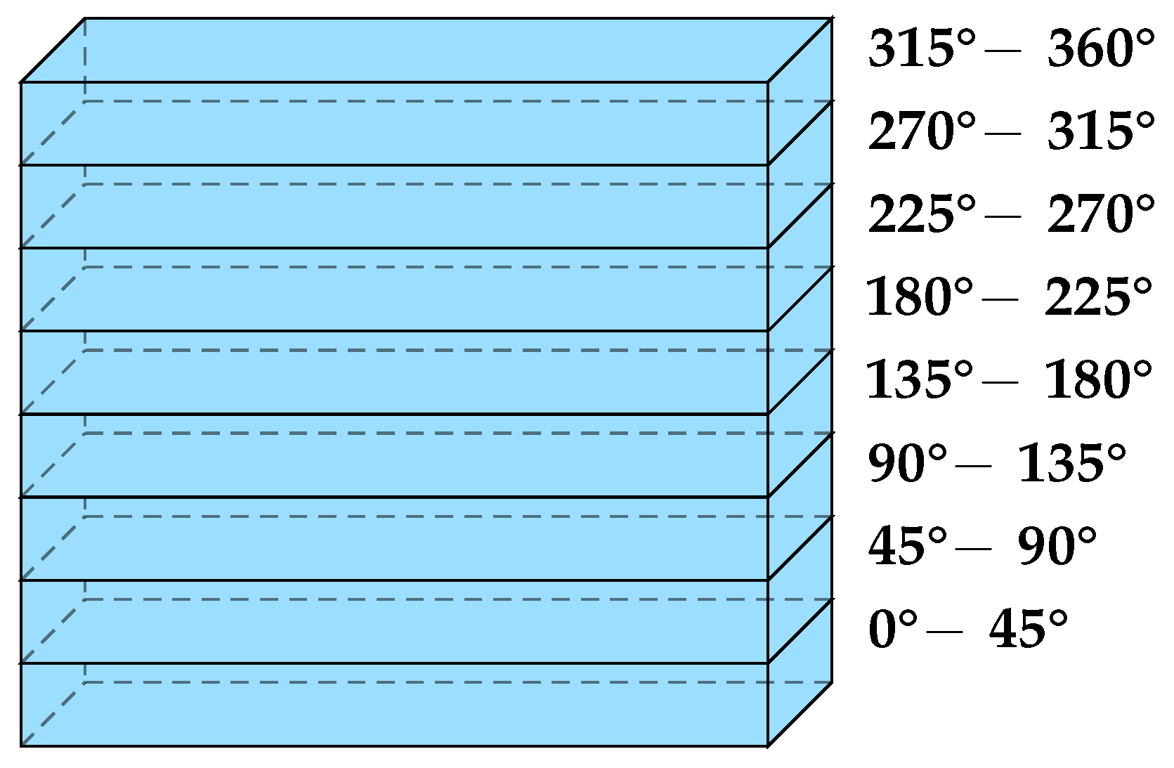