Stepwise Soft Actor–Critic for UAV Autonomous Flight Control

Abstract

Despite the growing demand for unmanned aerial vehicles (UAVs), the use of conventional UAVs is limited, as most of them require being remotely operated by a person who is not within the vehicle’s field of view. Recently, many studies have introduced reinforcement learning (RL) to address hurdles for the autonomous flight of UAVs. However, most previous studies have assumed overly simplified environments, and thus, they cannot be applied to real-world UAV operation scenarios. To address the limitations of previous studies, we propose a stepwise soft actor–critic (SeSAC) algorithm for efficient learning in a continuous state and action space environment. SeSAC aims to overcome the inefficiency of learning caused by attempting challenging tasks from the beginning. Instead, it starts with easier missions and gradually increases the difficulty level during training, ultimately achieving the final goal. We also control a learning hyperparameter of the soft actor–critic algorithm and implement a positive buffer mechanism during training to enhance learning effectiveness. Our proposed algorithm was verified in a six-degree-of-freedom (DOF) flight environment with high-dimensional state and action spaces. The experimental results demonstrate that the proposed algorithm successfully completed missions in two challenging scenarios, one for disaster management and another for counter-terrorism missions, while surpassing the performance of other baseline approaches.

1. Introduction

Unmanned aerial vehicles (UAVs) are used in diverse areas, such as entertainment (e.g., light shows), networking, smart agriculture, and missions that are dangerous or inaccessible to humans, including search and rescue, surveillance, blood transport, photogrammetry, natural disaster risk measurement, and counter-terrorism [1,2,3,4,5,6,7,8,9,10,11,12]. Although UAV control technology has steadily advanced in recent years, the main control methods still involve the use of wireless remote operation or preprogramming. With remote operation, there is a risk that the communication link may fail to work in real-time. Additionally, the controllable distance is limited. While there are no communication link limitations with the preprogramming option, it can only be applied to limited missions and cannot adapt to unexpected situations. To overcome these limitations and maximize the potential of UAVs, researchers have developed autonomous flight algorithms for UAVs [13,14,15].

UAVs can be divided into rotary-wing UAVs, flexi-wing UAVs, and fixed-wing UAVs. Rotary-wing UAVs fly using lift generated by the rotation of their blades. Rotary wings can take off and land vertically in small spaces and remain stationary in the air. Fixed-wing UAVs have wings that are fixed to the fuselage and utilize the lift generated by the pressure difference between the air above and below the wings to fly. They are relatively stable compared to rotary wings and capable of flying at high speeds and high altitudes. Due to these differences, fixed-wing UAVs are primarily used for military and surveillance purposes, where they are suitable for high-altitude and long-range missions [16,17]. Flexi-wing UAV refers to an aircraft where the shape of the wings changes during flight to optimize flight performance or achieve specific objectives. Various forms of modifications, such as wingspan, area, camber, chord, thickness, and aspect ratio, have been studied [18,19].

Researchers have long studied autonomous flight for fixed-wing UAVs in military aircraft. Their approaches range from rule-based techniques to reinforcement learning (RL) techniques. The traditional approach of autonomous flight for UAVs was based on the rule-based method, where experts determine the favorable actions for achieving a mission in a specific situation and subsequently plan rules to perform the corresponding maneuvers [20,21,22,23]. Because rule-based techniques enable aircraft to perform predetermined maneuvers under given conditions, it is difficult to respond appropriately to unexpected situations [24]. Hence, recent studies have utilized RL techniques that are particularly suited to learning to make decisions quickly in unpredictable or uncertain situations [25,26,27,28,29,30,31]. Masadeh et al. [6] utilized multi-agent deep deterministic policy gradient and Bayesian optimization to optimize the trajectory and network formation of UAVs for rapid data transmission and minimize energy consumption and transmission delay in a situation where multiple UAVs are used as repeaters in a wireless network. Gong et al. [11] developed an intelligent UAV that can detect dynamic intruder targets using RL. The performance of RL-based target detection using Sarsa, and Q-learning was found to be superior to the existing systems that perform random or circular target detection.

In the field of autonomous flight of fixed-wing UAVs, various studies have adopted RL techniques. For example, to simplify the action space, Yang et al. [28] trained a deep Q network (DQN) to select appropriate maneuvers for UAVs in dogfighting situations and showed successful results in simulated one-on-one short-range dogfights. However, it has the limitation of simplifying the maneuver space to 15 predefined maneuvers. Wang et al. [29] proposed a league system that can flexibly respond to various maneuvers of the enemy aircraft in a simulation environment where the speed of the aircraft is continuously limited, achieving a win rate of 44% and a probability of not losing 75%. However, the experimental environment is limited to 2D, which is difficult to apply to the actual environment. Lee et al. [30] introduced an enhanced version of self-imitation learning and a random network distillation algorithm. However, the experiment was performed in a 3 degrees of freedom (DOF) environment, which does not reflect realistic environments. Furthermore, several studies [31,32,33,34] have proposed RL-based techniques for chasing, landing, or maintaining the altitude of an aircraft under various flight conditions, but all experiments have either had a limited action space or were conducted in a simplified simulation environment. In summary, existing works need further verification in more diverse and realistic environments.

In a realistic 6-DOF flight environment, it is difficult to learn high-dimensional characteristics of the state and action spaces [35]. To overcome high dimensionality, Imanberdiyev et al. [36] proposed TEXPLORE, which improves the conventional model-based reinforcement learning using decision trees to learn the given environment model. It achieves the desired learning results in fewer epochs compared to the Q-learning. Wang et al. [37] introduce a method called nonexpert helper, where a pre-policy network provides guidance to the agent in exploring the state space. Wang et al. [38] have developed a deep reinforcement learning (DRL) framework for UAV navigation in complex environments with numerous obstacles. However, these studies focus on navigation rather than UAV control.

To address the limitations of previous studies on training fixed-wing UAVs for autonomous flight, we propose a novel learning method for UAV agents. First, for effectively learning high-dimensional state and action spaces, a positive buffer is added to the experience of past successes. Second, we apply a new technique that suppresses alpha, the temperature parameter that encourages exploration, after achieving the desired goal of maintaining the stable performance of the soft actor–critic (SAC) algorithm. Finally, we propose a novel stepwise SAC (SeSAC), which assigns easy missions at the beginning of training and then gradually increases the difficulty while training to reach the desired goal successfully.

The proposed algorithm was implemented in realistic simulation environments that we constructed using the 6-DOF flight dynamics model JSBSim [39], instead of using a simplified simulation environment. Specifically, we conducted experiments on two realistic scenarios, including disasters and counter-terrorism, to verify the effectiveness of the proposed approach. The experimental results show that the agent trained through the SeSAC successfully completed missions in two challenging scenarios, while outperforming other RL-based approaches.

The contributions of this paper are summarized as follows:

• In this study, we constructed realistic flight environments based on JSBSim, a 6-DOF flight environment with high-dimensional state and action spaces;
• We define states, actions, and rewards for the UAV agent to successfully accomplish disaster management and counter-terrorism missions. We incorporated past experiences by stacking the states of previous time steps into the states by utilizing a 1D convolution layer. Additionally, we customized the episode rewards and time step rewards to match the specific characteristics of each mission;
• We introduce a positive buffer and a cool-down alpha technique into the SAC algorithm to improve learning efficiency and stability;
• Finally, we propose SeSAC by incorporating the concept of stepwise learning. Throughout the experiments, it was confirmed that the agent trained with SeSAC succeeded in the mission with fewer learning epochs and a higher average reward.

The remainder of this paper is organized as follows. Section 2 provides an overview of the RL and SAC algorithms. In Section 3, we propose the SeSAC and define the UAV agent’s states, actions, and rewards. Section 4 describes the experimental scenarios and presents the results. Finally, Section 5 concludes this research and discusses future research directions.

2. Background

2.1. Reinforcement Learning

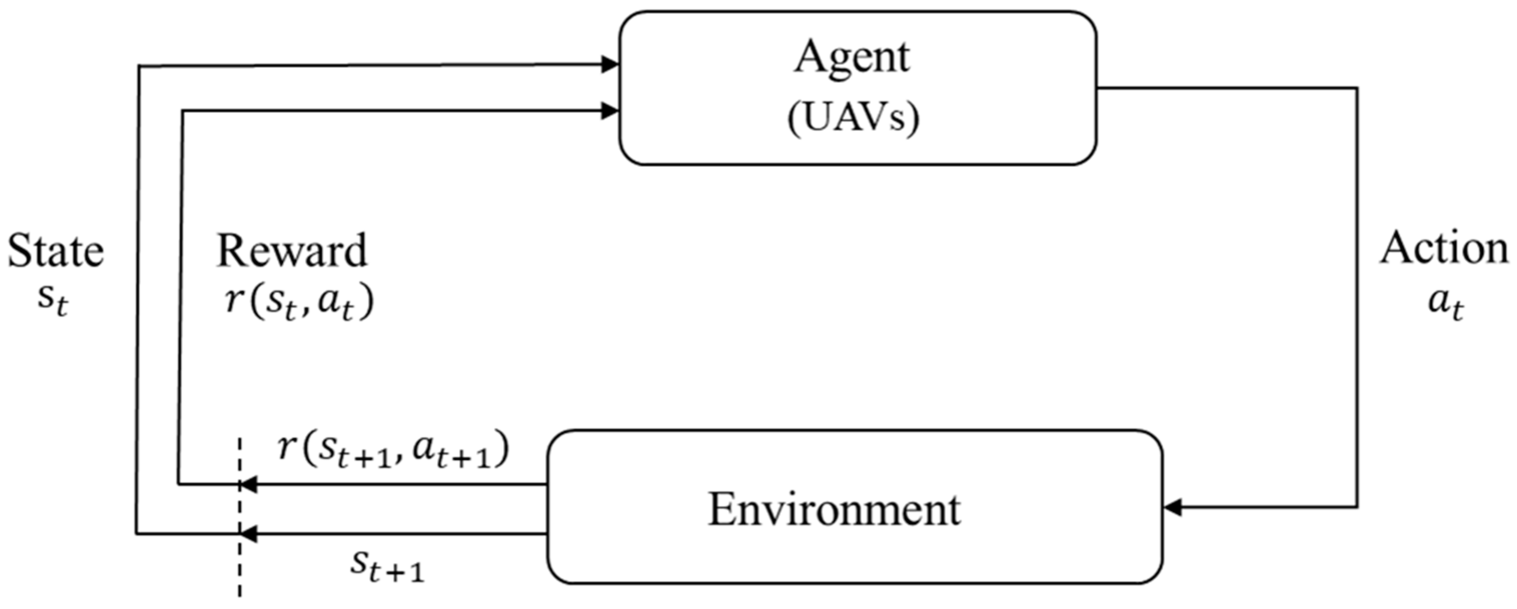
RL is an important field of machine learning that solves sequential decision-making problems [40]. In RL, an agent interacts with an environment. As illustrated in Figure 1, the agent takes actions based on a policy for a given state, and the environment responds with a reward for that action. RL repeatedly goes through this process to ultimately learn policy $\pi$, aiming for optimal decision-making. This process adheres to the “Markov property”, which implies that given the current state $S_t$, the history prior to that state does not provide any additional information about the next state $S_{t+1}$ or the reward $R_{t+1}$ [40]. Therefore, all the necessary information is encapsulated in the current state $S_t$, making the RL problem one where the agent learns the optimal policy within the structure of a Markov Decision Process (MDP).

In Figure 1, the agent and environment interact at each timestep. At time step $t$, the agent makes action $a_t$ based on state $s_t$ observed from the environment. Then, the next state, $s_{t+1}$, is stochastically determined, given $s_t$ and $a_t$, and the reward $r\left(s_t, a_t\right)$ is provided as a feedback from the environment. The agent repeats this process until a termination condition is met. The purpose of the RL algorithm is to find the optimal policy ${\pi }^{*}$ that maximizes the expected total reward at each timestep $t$, as shown in Equation (1). In Equation (1), $\gamma$ represents the discount rate, with a value between 0 and 1, where $\tau$ represents trajectories $\left(\left(s_1,a_1\right), \left(s_2,a_2\right), \cdots \right)$.

$${\pi }^{*}={argmax}_{\pi }\sum _t{E}_{\tau ~\pi } {\gamma }^{t-1}\left[r\left(s_t, a_t\right)\right].$$

(1)

2.2. Actor–Critic Algorithm

Based on the learning goal, RL algorithms can be categorized into value-based and policy-based algorithms [41]. Value-based algorithms focus on estimating the value of each state through a value function in order to choose the optimal action in a given state. By learning and updating the value function, the agent determines its behavior based on the expected return it can receive in the future. Policy-based algorithms focus on learning a policy by which the agent chooses actions directly. Typically, the policy is represented by a probability distribution for choosing each action in a given state, and when choosing an action in a given state, the agent probabilistically selects an action based on this function. The actor–critic algorithm combines the strengths of value-based and policy-based algorithms [42].

The actor–critic algorithm consists of an actor network that learns policies and a critic network that approximates the values of states. Specifically, the actor network incrementally learns better actions by updating its policies to maximize rewards, given the state value function estimated by the critic network [43]. In other words, the actor network and the critic network are updated alternately.

2.3. Soft Actor–Critic

The SAC algorithm was announced by Berkeley and DeepMind in 2018 [44]. It encourages exploration through entropy and improves learning efficiency by reusing learning data through a buffer [44]. The objective function to maximize in the SAC algorithm is defined as

$$J\left({\pi }_{\theta }\right)=\sum _t{E}_{\tau ~{\pi }_{\theta } }\gamma \left[r\right(s_t, a_t)+\alpha H\left({\pi }_{\theta }\left(·|s_t\right))\right],$$

(2)

where $\theta$ is the parameter set of the actor network, and $\alpha$ is the balancing parameter for the entropy term $H$ with larger values encouraging exploration. $\alpha$ is often called the temperature.

The SAC algorithm adds the term $H$ representing entropy to (1). The entropy term $H\left(\pi \left(·|s_t\right)\right)$ is introduced to encourage the agent’s exploration. This term enforces the probabilities of all actions occurring as equally as possible, thereby enabling the exploration of diverse action spaces to explore better policies and various optimal points [45].

3. Proposed Method

In this study, we propose a learning method to efficiently train an agent in an environment with continuous state and action spaces of the autonomous flight environments. Specifically, a positive buffer is additionally used in the SAC algorithm to use the experience of successful episodes. Furthermore, the cool-down alpha technique is introduced for learning efficiency and stability. Finally, a novel SeSAC is proposed to conduct learning incrementally from easy missions until the final goal is reached.

3.1. Positive Buffer

The SAC algorithm stores the experience of past episodes in the replay buffer in the form of a tuple $\left(s_t,a_t,r_t,s_{t+1}\right)$ to conduct off-policy learning [44]. In general, the experiences from episodes are stored in a replay buffer regardless of the success or failure of the episode, and a batch with a fixed size is randomly sampled from the replay buffer for training. Therefore, all experiences are sampled with equal probability without distinction between successful and unsuccessful episodes. However, if successful and unsuccessful episodes are clearly distinguished as UAV missions, the experience from successful episodes can be reflected in the early stages of learning to improve learning efficiency. With this aim, we create a positive buffer where the experience from successful episodes is stored separately and utilized for learning. As shown in Figure 2, the proposed model uses three memory buffers. The episode buffer serves as a temporary buffer, storing only tuples from a single episode, while the replay buffer retains all experiences. Once an episode is completed, tuples stored in the episode buffer are added to the positive buffer if the agent meets the success criteria score set by the hyperparameters. If the episode fails, these tuples are discarded. Each memory adopts a strategy of deleting the oldest tuples if the predefined memory size is exceeded. For training, data is randomly extracted in batch sizes from both the replay and positive buffers. In the early stages of training, if there are no successful episodes, sampling is conducted solely from the replay buffer. Once the size of the positive buffer exceeds the batch size, training samples are drawn from both the positive and replay buffers at a 3:1 ratio.

The bottom part of Figure 2 shows how SAC learns. The actor uses a Policy network to take a given state as input and output a probability for each action. The Critic consists of two main Q-networks and two corresponding target Q-networks. The main Q-networks perform training and constantly update the parameters ${\theta }_1$ and ${\theta }_2$ of each network, while the target Q-networks remain frozen by periodically copying the parameters ${\theta }_1$ and ${\theta }_2$ to ${\overline{\theta }}_1$ and ${\overline{\theta }}_2$. This allows the parameters of the network used to predict the target value to stabilize over time, increasing the consistency of the predictions and ensuring stable training.

3.2. Cool-Down Alpha

In SAC, the optimal policy ${\pi }^{*}$ is the one that maximizes the objective function defined in Equation (2) where $H\left(\pi \left(·|s_t\right)\right)$ is used to encourage exploration. It maximizes the entropy of the probabilities of all actions that can be selected in the current state $s_t$. Hence, with higher $\alpha$ values, it performs random actions, thereby encouraging exploration. On the other hand, at smaller values, exploitation is encouraged with the aim of maximizing the reward [44].

A high α can enhance an agent’s performance by promoting exploration in its initial stages during training when a good policy for mission completion is not obtained yet. However, a large α can compromise the stability of the learning process in its later stages following a successful mission. To address this issue, we apply ${\alpha }_{cool}$, the cool-down alpha, to maintain the learning process stable when the learned policy can be considered sufficiently good after a certain number of consecutive successful missions.

The above-described positive buffer and cool-down alpha were added to the SAC algorithm, which is represented in the pseudocode in Algorithm 1. Three values must be set before learning: $R_s, N_s, {\alpha }_{cool}$. $R_s$ is set as the value of the reward provided to the agent when it achieves the desired goal, which is the success criterion of the episode. $N_s$ is the threshold of the number of consecutive successful missions for applying ${\alpha }_{cool}$.

Algorithm 1: Soft Actor–Critic + Positive Buffer + Cool-down alpha

$1:\mathbf{S}\mathbf{e}\mathbf{t}:R_s,N_s, {\alpha }_{cool }$ $2:\mathbf{I}\mathbf{n}\mathbf{i}\mathbf{t}\mathbf{i}\mathbf{a}\mathbf{l}\mathbf{i}\mathbf{z}\mathbf{e} {\theta }_1, {\theta }_2, \varphi \hspace{1em}▷$Initialize main Q-network weights ${\theta }_1$, ${\theta }_2$ and policy network weight $\varphi$ $3:\hspace{1em} {\overline{\theta }}_1\leftarrow {\theta }_1, {\overline{\theta }}_2\leftarrow {\theta }_2\hspace{1em}\hspace{1em}\hspace{1em}\hspace{1em}\hspace{1em}\hspace{1em}\hspace{1em} ▷$Initialize target Q-network weights ${\overline{\theta }}_1$, ${\overline{\theta }}_2$ $4:\hspace{1em} {\mathcal{B}}_{\mathrm{R}}, {\mathcal{B}}_{\mathrm{P}}\leftarrow \mathrm{\varnothing }\hspace{1em}\hspace{1em}\hspace{1em}\hspace{1em}\hspace{1em}\hspace{1em}\hspace{1em}\hspace{1em}\hspace{1em}\hspace{1em}\hspace{1em} ▷$Initialize replay and positive buffer $5:\hspace{1em} R, N\leftarrow 0$ $6:\hspace{1em} \mathbf{F}\mathbf{o}\mathbf{r} each episode \mathbf{D}\mathbf{o}$ $7:\hspace{1em}\hspace{1em} {\mathcal{B}}_{\mathrm{E}}\leftarrow \mathrm{\varnothing }\hspace{1em}\hspace{1em}\hspace{1em}\hspace{1em}\hspace{1em}\hspace{1em}\hspace{1em}\hspace{1em}\hspace{1em}\hspace{1em}\hspace{1em}\hspace{1em}\hspace{1em}\hspace{1em}\hspace{1em}\hspace{1em} ▷$Initialize episode buffer $8:\hspace{1em}\hspace{1em} \mathbf{F}\mathbf{o}\mathbf{r} each timestep \mathbf{D}\mathbf{o}$ $9:\hspace{1em}\hspace{1em}\hspace{1em} a_t ~ {\pi }_{\varphi }\left(·|s_t\right)$ $10:\hspace{1em}\hspace{1em}\hspace{1em} s_{t+1}~ p\left(·\right|s_t, a_t)$ $11:\hspace{1em}\hspace{1em}\hspace{1em} {\mathcal{B}}_{\mathrm{R}}\leftarrow {\mathcal{B}}_{\mathrm{R}}\cup \left\{\left(s_t,{ a}_t,r_t,{ s}_{t+1}\right)\right\}$ $12:\hspace{1em}\hspace{1em}\hspace{1em} {\mathcal{B}}_{\mathrm{E}}\leftarrow {\mathcal{B}}_{\mathrm{E}}\cup \left\{\left(s_t,{ a}_t,r_t,{ s}_{t+1}\right)\right\}$ $13:\hspace{1em}\hspace{1em}\hspace{1em} R\leftarrow R+r_t$ $14:\hspace{1em}\hspace{1em} \mathbf{E}\mathbf{n}\mathbf{d} \mathbf{F}\mathbf{o}\mathbf{r}$ $15:\hspace{1em}\hspace{1em} \mathbf{I}\mathbf{F} R\ge R_s \mathbf{T}\mathbf{h}\mathbf{e}\mathbf{n}$ $16:\hspace{1em}\hspace{1em}\hspace{1em} {\mathcal{B}}_{\mathrm{P}}\leftarrow {\mathcal{B}}_{\mathrm{E}}$ $17:\hspace{1em}\hspace{1em}\hspace{1em} N \leftarrow N+1$ $18:\hspace{1em}\hspace{1em} \mathbf{E}\mathbf{n}\mathbf{d} \mathbf{I}\mathbf{F}$ $19:\hspace{1em}\hspace{1em} \mathbf{F}\mathbf{o}\mathbf{r} each gradient \mathrm{s}\mathrm{t}\mathrm{e}\mathrm{p} \mathbf{D}\mathbf{o}$ $20:\hspace{1em}\hspace{1em}\hspace{1em} {\theta }_i\leftarrow {\theta }_i-{\lambda }_Q {\nabla }_{{\theta }_i} J_Q\left({\theta }_i\right)\hspace{1em}\mathit{f}\mathit{o}\mathit{r} i\in \left\{\mathrm{1,2}\right\}\hspace{1em}\hspace{1em}\hspace{1em}▷$Update Q-function parameters $21:\hspace{1em}\hspace{1em}\hspace{1em} \varphi \leftarrow \varphi -{\lambda }_{\pi }{\nabla }_{\varphi }{J}_{\pi }\left(\varphi \right)\hspace{1em}\hspace{1em}\hspace{1em}\hspace{1em}\hspace{1em}\hspace{1em}\hspace{1em}\hspace{1em}\hspace{1em}\hspace{1em}\hspace{1em}\hspace{1em}▷$Update policy weights $22:\hspace{1em}\hspace{1em}\hspace{1em} {\overline{\theta }}_i\leftarrow {\tau \theta }_i+\left(1-\tau \right){\overline{\theta }}_i\hspace{1em}\mathit{f}\mathit{o}\mathit{r} i\in \left\{\mathrm{1,2}\right\}\hspace{1em}\hspace{1em}\hspace{1em}\hspace{1em}▷$Update target network weights $23:\hspace{1em}\hspace{1em}\hspace{1em} \mathbf{I}\mathbf{F} N\ge N_s \mathbf{T}\mathbf{h}\mathbf{e}\mathbf{n}$ $24:\hspace{1em}\hspace{1em}\hspace{1em}\hspace{1em} \mathsf{\alpha }\leftarrow {\alpha }_{cool}$ $25:\hspace{1em}\hspace{1em}\hspace{1em} \mathbf{E}\mathbf{L}\mathbf{S}\mathbf{E}$ $26:\hspace{1em}\hspace{1em}\hspace{1em}\hspace{1em} \mathsf{\alpha }\leftarrow \alpha -\lambda {\nabla }_{\alpha } J\left(\alpha \right)\hspace{1em}\hspace{1em}\hspace{1em}\hspace{1em}\hspace{1em}\hspace{1em}\hspace{1em}\hspace{1em}\hspace{1em}\hspace{1em}▷$Adjust temperature parameter $27:\hspace{1em}\hspace{1em}\hspace{1em}\hspace{1em} where, J\left(\alpha \right)=E_{a_t~{\pi }_t }\left[-\alpha \log {\pi }_t\left(a_t|s_t\right)-\alpha \overline{\mathcal{H}}\right]$ $28:\hspace{1em}\hspace{1em}\hspace{1em} \mathbf{E}\mathbf{n}\mathbf{d} \mathbf{I}\mathbf{F}$ $29:\hspace{1em}\hspace{1em} \mathbf{E}\mathbf{n}\mathbf{d} \mathbf{F}\mathbf{o}\mathbf{r}$ $30:\hspace{1em} \mathbf{E}\mathbf{n}\mathbf{d} \mathbf{F}\mathbf{o}\mathbf{r}$ $31:\mathbf{O}\mathbf{u}\mathbf{t}\mathbf{p}\mathbf{u}\mathbf{t}: {\theta }_1, {\theta }_2, \varphi$

3.3. Stepwise Soft Actor–Critic

In the proposed SeSAC learning process, we gradually elevate the criteria for successful completion of the episode, thereby training the agent in the desired direction. Specifically, our proposed SeSAC performs learning by initially relaxing the termination conditions to allow for easy mission success and gradually increasing the difficulty of these conditions to reach the desired goal. This approach enables the agent to progressively accomplish the desired objective, beginning with a lower difficulty level.

Let $G_{final}, G,$ and $C$ represent the level of the final goal, the level of the initial goal, and the margin level increase for each step, respectively. Algorithm 2 shows the pseudocode of our proposed SeSAC algorithm. In this algorithm, once the agent completes learning for the current goal, $G$, the difficulty of the mission is increased by $C$ step by step until it reaches $G_{final}$, and learning continues until the final goal is achieved. An episode is deemed successful if the cumulative reward for that episode exceeds $R_s$, the threshold for episode success. Furthermore, if $N$ consecutive episodes are successful, it is assumed that learning for that level is complete, and the difficulty is escalated to proceed with the next level of learning. In the example depicted in Figure 3, the final goal is set as a target radius of 0.1 km, the initial goal is set as 1.0 km, and $C$ (difficulty increment) is set as −0.1 km.

Algorithm 2: Stepwise soft actor–critic (SeSAC)

$1:\hspace{1em}\mathbf{S}\mathbf{e}\mathbf{t} G_{final}, G, C, N, R_s$ $2:\hspace{1em}\mathbf{I}\mathbf{n}\mathbf{i}\mathbf{t}\mathbf{i}\mathbf{a}\mathbf{l}\mathbf{i}\mathbf{z}\mathbf{e} N_C=0, G=G_{initial}$ $3:\hspace{1em}\mathbf{F}\mathbf{o}\mathbf{r} each episode \mathbf{D}\mathbf{o}$ $4:\hspace{1em}\hspace{1em}\mathbf{I}\mathbf{F} G \ne G_{final} \mathbf{D}\mathbf{o}$ $5:\hspace{1em}\hspace{1em}\hspace{1em}R\leftarrow 0$ $6:\hspace{1em}\hspace{1em}\hspace{1em}\hspace{1em} \mathbf{F}\mathbf{o}\mathbf{r} each timestep \mathbf{D}\mathbf{o}$ $7:\hspace{1em}\hspace{1em}\hspace{1em}\hspace{1em}\hspace{1em}\hspace{1em}{a}_t ~ \pi \left(·|s_t\right)$ $8:\hspace{1em}\hspace{1em}\hspace{1em}\hspace{1em}\hspace{1em}\hspace{1em}{s}_{t+1}~ p\left(·\right|s_t, a_t)$ $9:\hspace{1em}\hspace{1em}\hspace{1em}\hspace{1em}\hspace{1em}\hspace{1em}R\leftarrow R+r_t$ $10:\hspace{1em}\hspace{1em}\hspace{1em}\hspace{1em} \mathbf{E}\mathbf{n}\mathbf{d} \mathbf{F}\mathbf{o}\mathbf{r}$ $11:\hspace{1em}\hspace{1em}\hspace{1em}\hspace{1em} \mathbf{I}\mathbf{f} R\ge R_s \mathbf{T}\mathbf{h}\mathbf{e}\mathbf{n}$ $12:\hspace{1em}\hspace{1em}\hspace{1em}\hspace{1em}\hspace{1em}\hspace{1em}{N}_C\leftarrow N_C+1$ $13:\hspace{1em}\hspace{1em}\hspace{1em}\hspace{1em} \mathbf{E}\mathbf{l}\mathbf{s}\mathbf{e}$ $14:\hspace{1em}\hspace{1em}\hspace{1em}\hspace{1em}\hspace{1em}\hspace{1em}{N}_C\leftarrow 0$ $15:\hspace{1em}\hspace{1em}\hspace{1em}\hspace{1em} \mathbf{E}\mathbf{n}\mathbf{d} \mathbf{I}\mathbf{f}$ $16:\hspace{1em}\hspace{1em}\hspace{1em}\hspace{1em} \mathbf{I}\mathbf{f} N_C=N \mathbf{T}\mathbf{h}\mathbf{e}\mathbf{n}$ $17:\hspace{1em}\hspace{1em}\hspace{1em}\hspace{1em}\hspace{1em}\hspace{1em}G\leftarrow G+C$ $18:\hspace{1em}\hspace{1em}\hspace{1em}\hspace{1em} \mathbf{E}\mathbf{n}\mathbf{d} \mathbf{I}\mathbf{f}$ $19:\hspace{1em}\hspace{1em}\mathbf{E}\mathbf{l}\mathbf{s}\mathbf{e}$ $20:\hspace{1em}\hspace{1em}\hspace{1em}\mathbf{B}\mathbf{r}\mathbf{e}\mathbf{a}\mathbf{k}$ $21:\hspace{1em}\hspace{1em}\mathbf{E}\mathbf{n}\mathbf{d} \mathbf{I}\mathbf{f}$ $22:\hspace{1em}\mathbf{E}\mathbf{n}\mathbf{d} \mathbf{F}\mathbf{o}\mathbf{r}$

3.4. Environment and Agent Design

3.4.1. Environment

In this study, the UAV is implemented on JSBSim, an open-source flight dynamics model [39]. JSBSim is a lightweight, data-driven, nonlinear, 6-DOF open-source flight dynamics model that allows for sophisticated flight dynamics and control. Aircraft types and their equipment, such as engines and radar, are modeled in extensible markup language, so that they can be simply modeled in comparison to existing models. Hence, it has been used in various applications, including flight design, spacecraft, and missile design [30]. In addition, due to these advantages, JSBSim is applied for a variety of purposes in RL studies that require a sophisticated simulation environment. One major example is the air combat evolution program, supervised by the US Defense Advanced Research Projects Agency [25]. JSBSim was developed in C++, but for suitable adaptability in a Python environment, we modified the JSBSim-Wrapper developed in [46] to suit the experimental environment in this study.

JSBSim-Wrapper defines 51 types of information about aircraft position, speed, engine status, and control surface positions, such as aileron and rudder, among the data generated by JSBSim. For this study, 10 states were selected from this information, and an additional 8 states were calculated based on the information about the target, resulting in a total of 18 states utilized for the learning process. Moreover, from the 57 aircraft options provided by JSBSim, an INS/GPS-equipped fixed-wing aircraft was chosen as the agent for the experiments. The experiments were conducted using JSBSim’s default atmospheric environment, which is modeled based on the 1976 U.S. Standard Atmosphere and assumes no meteorological phenomena such as clouds or rainfall. The key libraries used in this study include Python 3.8.5, JSBSim 1.1.5, PyTorch 1.9.0, and Gym 0.17.2.

3.4.2. States

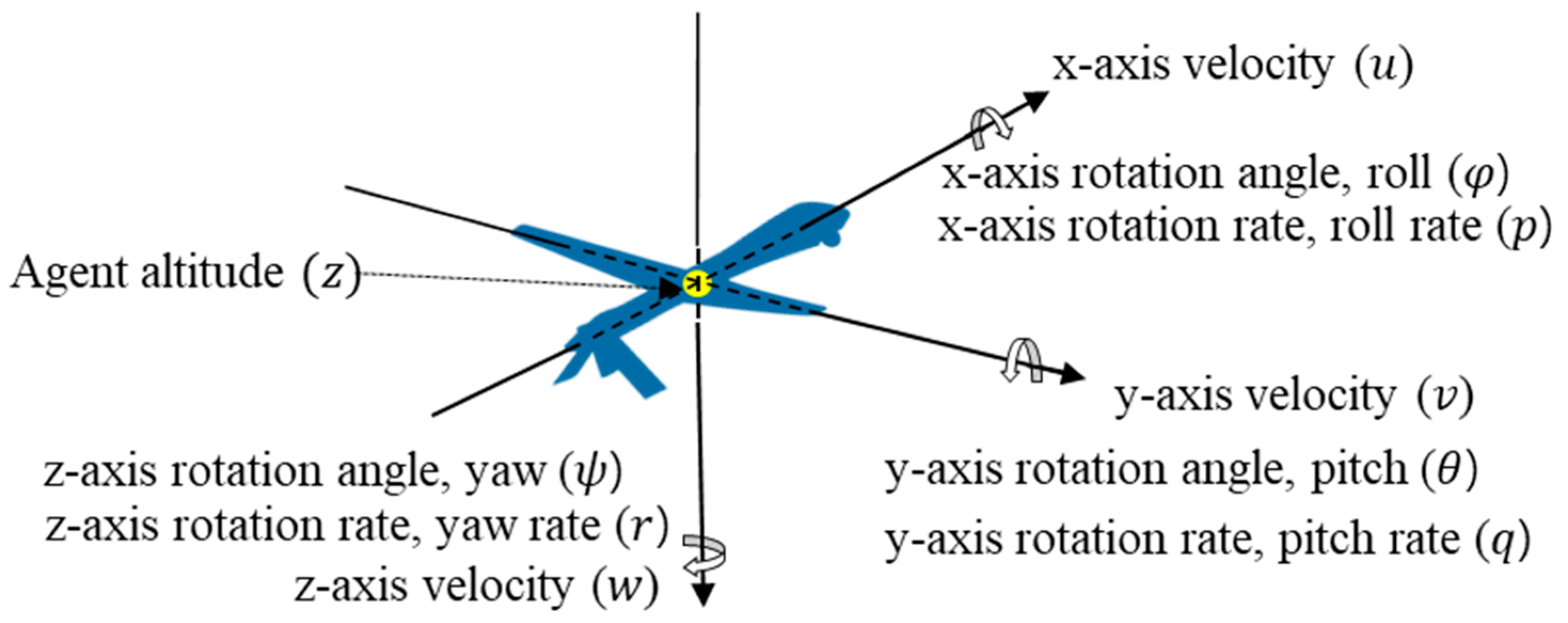
The states are represented by the finite set $S$. Each state must be obtainable from the environment and should contain the information required to learn the agent [47]. In this study, we combine $S_{basic}$, which includes the location and flight dynamics information of the agent directly obtainable from JSBSim, and $S_{relative}$, which includes the relative geometrical relationship with the target. Specifically, the state of the agent at timestep $t$ is as follows:

$$\begin{array}{c}{S}_t=\left\{S_{basic}, S_{relative}\right\},\\ \mathrm{w}\mathrm{h}\mathrm{e}\mathrm{r}\mathrm{e} S_{basic}=\left\{z_t, {\phi }_t, {\psi }_t,{\theta }_t, u_t, v_t, w_t, p_t, q_t, r_t\right\} \mathrm{a}\mathrm{n}\mathrm{d}\\ S_{relative}=\left\{D{x}_t,D{y}_t,D{z}_t,D_t,P_t,H_t, A{A}_t, HC{A}_t\right\}.\end{array}$$

(3)

Figure 3 shows $S_{basic}$, the agent’s information that it receives from JSBSim, and

Table 1. State definitions.

State	Definition	State	Definition
$z$	z-axis position	$r$	z-axis rotation rate
$\phi$	x-axis rotation angle	$Dx$	Difference in x-axis position
$\theta$	y-axis rotation angle	$Dy$	Difference in y-axis position
$\psi$	z-axis rotation angle	$Dz$	Difference of z-axis position
$u$	x-axis velocity	$P$	Pitch angle to target
$v$	y-axis velocity	$H$	Heading angle to target
$w$	z-axis velocity	$D$	Distance between agent and target
$p$	x-axis rotation rate	$AA$	Aspect angle
$q$	y-axis rotation rate	$HCA$	Heading cross angle

shows the definition of all elements of the state. In $S_{basic}$, the position of the agent is not used because we utilize its relative position to the target in $S_{relative}$. However, the altitude of the agent is important information for performing maneuvers, so $S_{basic}$ includes agent’s altitude $z$.

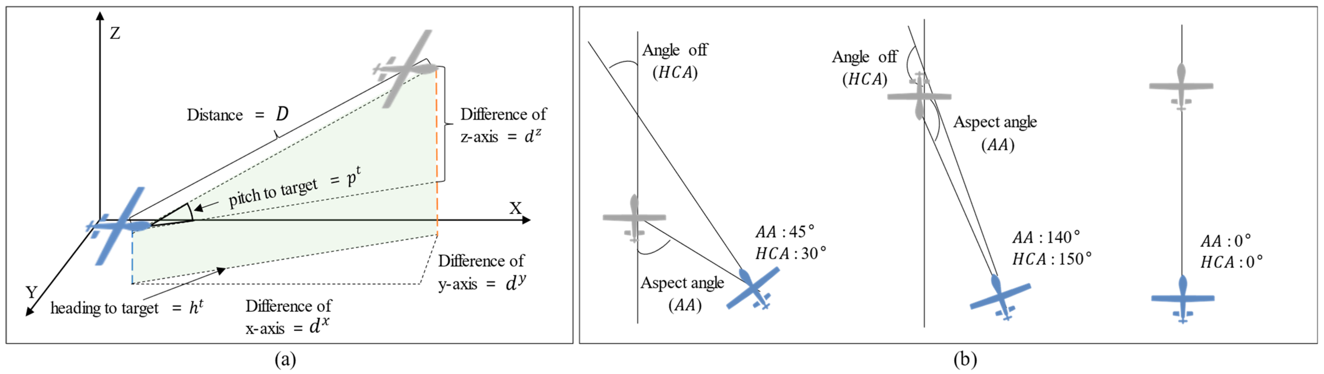
Figure 4 presents a detailed overview of each element. The aspect angle ($AA$) is the angle from the tail of the target, and the heading cross angle ($HCA$) is the heading difference between the two UAVs. If $AA$ and $HCA$ are known, then the vectors of the two aircraft can be expressed on a two-dimensional plane, as shown in Figure 4.

In this study, the 18 states defined above were stacked for 15 timestep states into one observation, and we applied a one-dimensional convolutional layer (1D CONV) to incorporate the agent’s past information into the input state and reduce the number of parameters, as shown in Figure 5. This new input state to the network is denoted by $s_t^s$ and is defined as follows

$$s_t^s={\sum }_{i=0}^{14}{w}_i{s}_{t-i},$$

(4)

where $w_i$ is the weights for 1D CONV kernel for time step $t-i$.

1D CONV is commonly employed for analyzing and processing sequential data such as signals and speech [48]. We utilized 1D CONV to compress the information, encompassing not only the agent’s current state but also the states from a specific time period in the past, in order to construct the input state.

3.4.3. Actions

The type of agent in this paper is a fixed-wing UAV. Hence, the action vector consists of the stick position $s_x,s_y$ and rudder pedal angle $\rho$, which controls the control surface, allowing the aircraft to move, and the throttle angle $\tau$, which controls the aircraft’s thrust (see

Table 2. Definition of actions.

Action	Definition	Action	Definition
$s_x$	X-axis stick position (−1–1)	$\tau$	Throttle angle (0–1)
$s_y$	Y-axis stick position (−1–1)	$\rho$	Rudder pedal angle (−1–1)

). The action at time step $t$ is defined as

$$a_t=\left(s_x, s_y, \tau , \rho \right)$$

(5)

3.4.4. Reward

The agent evaluates its action based on the given reward and learns to maximize the sum of expected future rewards. Thus, providing an appropriate reward according to the achievement of the agent is critical for successful learning [49]. We categorize the rewards into success rewards, failure rewards, and timestep rewards. Success rewards are given once the agent achieves the mission objective at the end of the episode. Failure rewards are received at the end of the episode if the agent fails to achieve the goal and crashes to the ground or overtakes the target, which means the mission has failed. Timestep rewards are given at each timestep to address the sparse reward problem in which the agent cannot be effectively trained due to lack of supervision when rewards are given sparsely (e.g., episodic rewards that are given only after an episode ends). Timestep rewards include

• Distance reward: Reward for the difference between the distance from the target at timestep $t-1$ and the distance from the target at timestep $t$. This induces the agent to approach the target without moving away from it;
• Line-of-sight (LOS) reward: Reward increases as the agent’s heading direction accurately faces the target in three-dimensional space. It consists of the pitch score and heading score, which are calculated based on the pitch angle and heading angle to the target, respectively.

The detailed definitions of success, failure, and timestep rewards will be described in the experimental design section of Section 4, as it is necessary to tailor the rewards to align with the specific characteristics of the mission.

4. Experiments

4.1. Experiment Design

To verify the effects of SeSAC, positive buffer, and cool-down alpha, we conducted comparative experiments on two baseline models, proximal policy optimization (PPO) [50] and SAC, as well as SAC + positive buffer (SAC-P), SAC-P + cool-down alpha (SAC-PC), and SAC-PC + stepwise learning (SeSAC). Here, the PPO is a policy-based algorithm proposed by OpenAI and widely used in various research and applications. The main objective of PPO is to maintain the similarity between the new policy and the previous policy during learning to ensure stability. The “proximity” condition in PPO prevents large updates in the policy, leading to improved stability and data efficiency [50].

In this study, we constructed experimental environments with two different missions. A precise approach mission (PAM) assumes a situation in which the agent must access a precise point to enter the disaster site or perform firefighting activities. The goal is to precisely approach a fixed target. As shown in Figure 6, the agent starts level and straight flight at an altitude of 25,000 feet and a speed of 300 knots with a bank angle of 0 degrees. The episode ends when the agent collides with the ground or approaches the target, 7.8 km away at a height of 500 ft. We assume that the goal is achieved if the agent is within 0.1 km of the target.

A moving target chasing mission (MTCM) is a counter-terrorism mission to track unlicensed aircraft approaching an airport or a defense maneuver scenario to protect important assets, in which the goal is to approach the moving target at a distance that can reduce the threat. The agent starts level and straight flight at an altitude of 25,000 feet and a speed of 300 knots with a bank angle of 0 degrees. The episode ends when the agent collides with the ground or approaches the circling target, which is 5.0 km away at a height of 500 ft. In this mission, it is assumed that the goal is achieved if the agent maintains within 12 degrees of $AA\&HCA$ for five consecutive timesteps and stays within 2.4 km of the target’s rear.

4.1.1. Reward Function for PAM

The reward function for PAM comprises three components: two episodic rewards—success reward and failure reward—and a distance reward, given at each time step.

• Success reward: This reward represents the success condition of the mission and is given as a reward of 500 when $D_t<0.1 \mathrm{k}\mathrm{m} \mathrm{a}\mathrm{n}\mathrm{d} {Dz}_t<0.1 \mathrm{k}\mathrm{m}$;
• Failure reward: This reward is received by −100 when $z_t<0.1 \mathrm{k}\mathrm{m} \mathrm{o}\mathrm{r} {\mathit{AA}}_t>90°$, which means the agent failed the mission by colliding with the ground or overtaking the target;
• Distance reward: The agent receives a value of $D_{t-1}-D_t$ at every timestep. This reward becomes negative when the agent is farther away from the target and positive when it is closer.

4.1.2. Reward Function for MTCM

The reward function for MTCM was composed of two episodic rewards and two timestep rewards by adding an LOS reward for continuous guidance in the direction of the moving target.

• Success reward: This reward of 100 is given when $D_t<2.4 \mathrm{k}\mathrm{m} \mathrm{a}\mathrm{n}\mathrm{d} AA<12° \mathrm{a}\mathrm{n}\mathrm{d} HCA<12°$. Additionally, if the agent satisfies these conditions consecutively for five timesteps, it is considered a success.
• LOS reward: As the agent’s gaze moves further away from the target, it receives a smaller reward, as follows

  $$\begin{array}{c}LOS reward=pitch reward+heading reward,\\ \mathrm{W}\mathrm{h}\mathrm{e}\mathrm{r}\mathrm{e} pitch reward=\left(0.3 \exp (-0.5{\left(\frac{P_t-{\theta }_t}{3°}\right)}^2\right),\\ \mathrm{a}\mathrm{n}\mathrm{d} heading reward=\left(0.3 \exp (-0.5{\left(\frac{H_t-{\psi }_t}{3°}\right)}^2\right).\end{array}$$

  (6)
• Failure and Distance reward: Same as PAM’s Failure and Distance reward.

4.1.3. Model Structure and Hyperparameters

The model for the experiment of the proposed method is based on the actor–critic algorithm, which consists of an actor and critic network. The model structure and the set of hyperparameters are shown in

Table 3. Model structure and hyperparameters.

Hyperparameter	Value	Hyperparameter	Value
Optimizer	Adam	$\tau$	${10}^{-4}$
The learning rate for actor network	${10}^{-4}$	Activation function	SeLU
The learning rate for critic network	${10}^{-3}$	Replay buffer capacity	${10}^5$
Batch size	128	Positive buffer capacity	${10}^5$
Configuration of hidden layers	[128, 64, 32, 32]

.

For SeSAC, the difficulty gradually increased from the initial goal to the final goal, as shown in Figure 7. Specifically, in the PAM, we set the success condition for the initial goal to the target radius of 2.0 km. If it succeeds at least five times consecutively, then the target’s radius is reduced by 0.1 km so that it reaches the final goal of 0.1 km after 20 steps. For the MTCM, we set the success condition for the initial goal to be 3.5 km behind the target with $AA\&HCA$ of 45°. If it succeeds in the mission 10 times consecutively, then the distance is reduced by 0.1 km, and the $AA\&HCA$ is reduced by 3°, so that it reaches the final goal of 2.4 km after 12 steps.

Table 4. Hyperparameters for stepwise soft actor–critic.

Hyperparameter	PAM	MTCM
$N_s$	50	50
${\alpha }_{cool}$	0.01	0.01
$R_s$	490	490
$G_{final}$	Target radius: 0.1 km	Target distance: 2.4 km, $AA\&HCA$: 12°
$G$	Target radius: 2.0 km	Target distance: 3.5 km, $AA\&HCA$: 45°
$C$	Target radius: −0.1 km	Target distance: −0.1 km, $AA\&HCA$: −3°
$N$	Five episodes	Ten episodes

shows the hyperparameters $N_s, {\alpha }_{cool}, R_s$ set in Algorithm 1 and $G_{final}, G, C, N, R_s$ set in Algorithm 2.

4.2. Experiment Results

4.2.1. Result for PAM

Table 5. Comparison results of baseline models on PAM.

	Min Score	Max Score	Mean Score	Cumulative Successes
PPO	−555.33	−47.91	−68.96	0
SAC	−133.42	509.82	−9.73	9
SAC-P	−124.53	510.20	−64.85	17
SAC-PC	−134.33	511.00	−64.03	62
SeSAC (entire)	−157.05	509.85	274.33	1781
SeSAC (final goal)	−157.05	509.85	338.31	1640

presents the results of PPO, SAC, SAC-P, SAC-PC, and SeSAC for the PAM scenario. The score refers to the sum of rewards received by the agent in one episode. In the PAM scenario, if the agent successfully accomplishes the mission, it receives a reward of 500. However, if the mission fails, it receives a reward of −100. Additionally, at each timestep, the agent receives a distance reward based on how far or close it is to the target. If the agent consistently moves away from the target, leading to a mission failure, it will receive a large negative score. The “Min score” and “Max score” columns indicate the lowest and highest scores achieved in individual episodes, respectively. The “Mean score” column represents the average score calculated from 3000 episodes, reflecting higher values when there are more successful episodes or when the agent shows progress in the desired direction. The “Cumulative successes” column refers to the total number of successful episodes accumulated during the 3000 episodes. Cumulative successes, along with the mean score, serve as indicators to assess the achievement of stable learning.

Unlike other experiments, the SeSAC experiment is presented in two parts: SeSAC (entire), which covers all 3000 episodes from the initial goal, and SeSAC (final goal), which is the result after the 842nd episode when the target radius of 0.1 km is reached. PPO failed to accomplish the mission in 3000 episodes and performed poorly across all metrics compared to the naive SAC. SAC-P and SAC-PC had lower average scores but outperformed SAC in terms of cumulative successes. These results can be interpreted as the increased success rates being attributed to the utilization of successful experiences stored in the positive buffer. In the case of SAC-PC, the cumulative number of successful episodes exceeded the threshold set by the cool-down alpha, indicating that the influence of cool-down alpha also played a role in the experiment. SeSAC, which combines SAC-PC with stepwise learning, demonstrated superior performance compared to other methods. After 842 episodes, SeSAC successfully reached the final goal of 0.1 km, with a total of 1640 successes since then.

Figure 8 shows the change in the cumulative rewards per episode. The proposed SeSAC achieved a stable score of at least 490 after about 1600 episodes, while learning was unsuccessful with the other comparison models. In Figure 8, the black dashed line shows the scores for the SeSAC model as the difficulty of the mission success criteria gradually increases from an initial target radius of 2.0 km to a final target radius of 0.1 km. All other solid lines, including the red solid line representing SeSAC, show scores at the final target radius of 0.1 km. Due to the progressive increase in the difficulty of SeSAC, we can observe significant fluctuations in the score plot. It shows a pattern where the agent repeatedly experiences failures after successfully completing the mission at a lower difficulty level when facing higher difficulty levels. PPO showed the lowest score among the other models. Furthermore, when comparing the naïve SAC with the advanced techniques proposed in this paper, it was challenging to observe significant differences in performance in this experiment. This means that the objective of PAM, which requires precise reaching of specific points in a 3D space, is difficult to achieve without stepwise learning. However, SAC-PC showed a trend of improving scores around the 2000th episode, indicating a potential for success. This suggests that the positive buffer and cool-down alpha play a role in enhancing the performance of SAC-PC.

Figure 9 details the relationship between the target radius, which represents difficulty, and the score of the SeSAC in the PAM mission, where the red solid line represents the target radius, and the difficulty increases gradually as the target radius decreases from the initial goal of 2.0 km to the final goal of 0.1 km. The initial goal of reaching a target radius of 2.0 km was achieved after 258 episodes, and from there, the difficulty continued to increase until reaching a target radius of 0.5 km. Accomplishing the 0.5 km target required a relatively long time. By comparing the score plot represented by the black dashed line and target radius, we observed that during the episode range of 200th to 400th, where the agent consistently achieved the objectives and faced increasing difficulty, high scores were obtained. The final goal of reaching a target radius of 0.1 km was achieved in episode 842, and after a series of successes and failures, it converged to a relatively stable score after episode 1500. The agent demonstrated a stepwise learning approach, leveraging the experiences learned in previous stages to rapidly increase the difficulty. Despite encountering periods of stagnation during the learning process, as evident from the score graph, the agent exhibited a pattern of alternating between failure and success, ultimately leading to successful learning and progression to the next stage.

Figure 10 shows a 3D plot of the learning process of the SeSAC algorithm for PAM. The blue solid line is the path of the agent, and the red circle is the target radius that the agent needs to reach. At the beginning of the training, the agent aims at an easy target with a wide range, but as the agent succeeds in the mission consecutively, the radius gradually decreases.

4.2.2. Result for MTCM

The MTCM experiment was conducted on a moving target. To complete the mission, the agent must stay within 2.4 km of the target for five consecutive timesteps while maintaining an $AA$ and $HCA$ within 12 degrees. For the SeSAC experiment, which required a change in difficulty, the initial target was set to a target distance of 3.5 km and an $AA$ and $HCA$ of 45 degrees, as shown in Figure 6, and the target distance was reduced by 0.1 km and the $AA$ and $HCA$ by 3 degrees after 10 consecutive successful missions.

Table 6. Comparison results of baseline models on MTCM.

	Min Score	Max Score	Mean Score	Cumulative Successes	First Convergent Episode
PPO	−2303.86	72.70	−359.96	2	-
SAC	−665.86	984.03	−296.78	22	-
SAC-P	−728.24	1829.24	95.21	1387	1602
SAC-PC	−638.35	1120.11	28.62	1246	1951
SeSAC (entire)	−650.34	928.17	404.90	2584	660
SeSAC (final goal)	−391.14	927.32	505.99	2308	660

shows the experimental results of our proposed models and comparative models for MTCM. The experimental results consist of the minimum, maximum, and mean scores of each experiment for 3000 episodes, cumulative successes, and the first convergent episode. The score represents the sum of rewards received in an episode, and cumulative success indicates the number of successful episodes out of 3000, serving as a metric for learning stability. The first convergent episode refers to how quickly the desired objective was achieved, representing the efficiency of learning. Here, the first convergent episode to identify the convergence point of the learning method was obtained following:

$$Convergent criteria=\sum _{i=0}^{50}(R_{t-i}-R_s)<\frac{R_s}{2},a_t=\left(s_x, s_y, \tau , \rho \right),$$

(7)

where $R_t$ is episode score of timestep $t$ and $R_s$ is the success criterion of the episode, which was set to 490 in the experiment.

The experimental results indicate that PPO and SAC, similar to the results of PAM, were unable to successfully complete the mission. On the other hand, SAC-P, SAC-PC, and SeSAC, which applied positive buffers, were able to achieve high average scores and succeed in more than 1000 episodes. Although SAC-PC, which introduced cool-down alpha, took about 350 episodes longer than SAC-P to converge to the desired score, a comparison of the plots of SAC-P represented by the green solid line and SAC-PC represented by the gold solid line in Figure 11 after the 1500th episode reveals that the introduction of cool-down alpha contributes to increased stability of the agent after achieving the desired score.

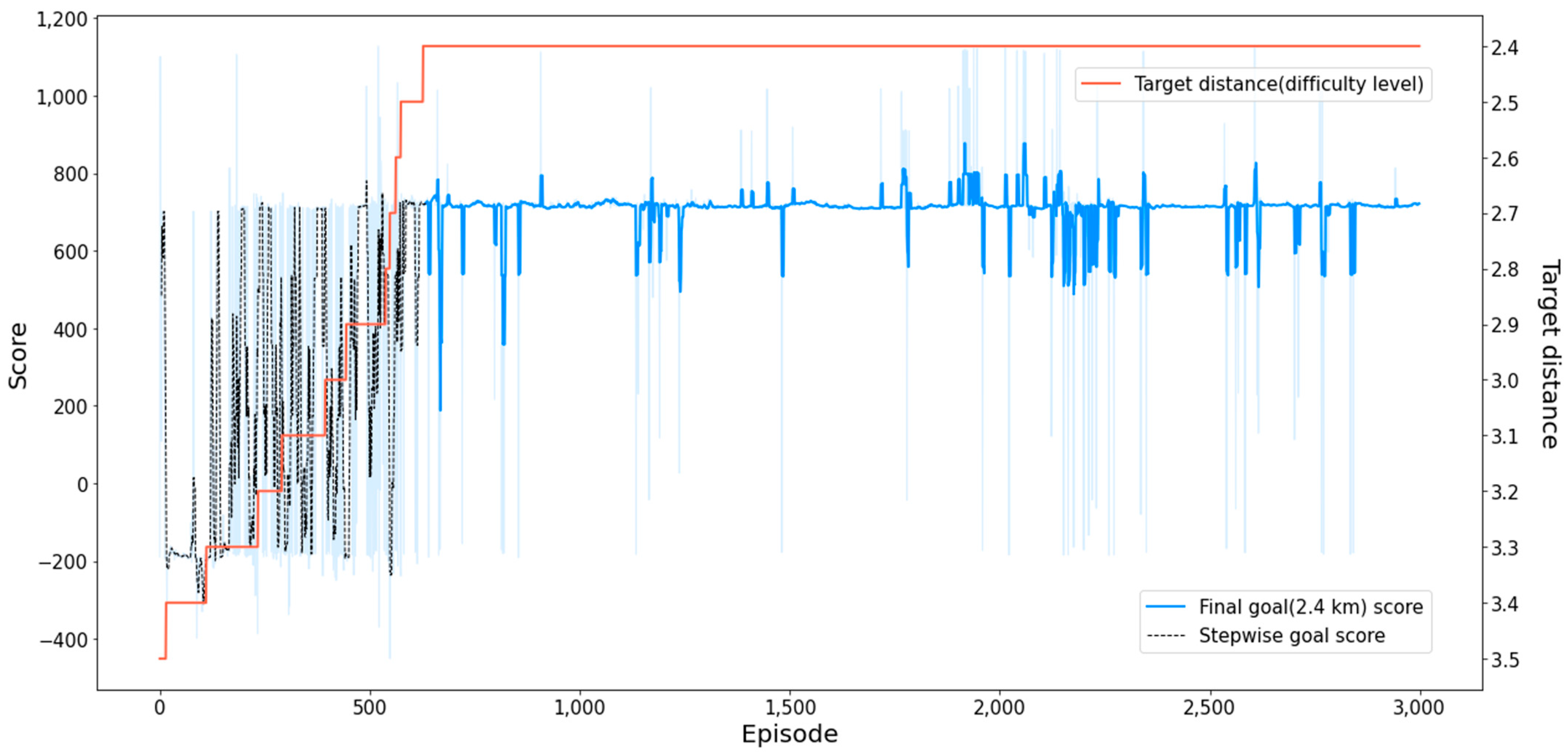
SeSAC showed overwhelming results in the mean score, cumulative success, and first convergent episode compared to other comparison methods. In particular, SeSAC showed superior performance in both cumulative successes and the first convergent episode compared to other methods, with over 1000 episodes of higher performance in each case. Also, after converging on the target score at episode 660, the score remained stable, influenced by the cool-down alpha. Figure 12 provides a more distinct depiction of the experimental results for MCTM. SeSAC demonstrated notably faster convergence than other methods, with a stable score after convergence. This highlights the clear superiority of the proposed method.

To verify the training process of SeSAC in detail, Figure 12 and Figure 13 present the scores for each episode and the movement path of the agent, respectively. In Figure 13, the red and blue lines represent the movement paths of the target and the agent, and the cone shape at the rear of the target shows the target that the agent needs to reach. As shown in Figure 13, the agent adapted to the increasing difficulty by learning step by step through the SeSAC algorithm, and after 627 episodes, it succeeded in reaching the final goal of a target distance of 2.4 km and $AA$&$HCA$ within 12 degrees.

5. Conclusions

In this study, we have developed a new training method, SeSAC, for efficient learning of fixed-wing UAVs in continuous state and action space environments. SeSAC performs stepwise learning, starting from easier missions, to overcome the inefficiency of learning caused by attempting challenging tasks from the beginning. We also added a positive buffer to utilize experiences from successful missions and controlled the hyperparameter that determines the amount of exploration in the SAC algorithm to enable stable learning. Furthermore, to effectively train the agent in a 6-DOF environment, we designed optimal states, actions, and rewards and integrated past states into the learning process using a 1D convolutional layer.

Experiments were conducted in two scenarios: the precision approach mission and the moving target-chasing mission. The proposed SeSAC approach demonstrated superior performance compared to PPO and conventional SAC, not only in terms of scores but also in the total number of successful episodes and first convergence episodes, indicating faster convergence and stable learning results. In particular, when using the First convergent episode as an indicator to assess the efficiency of learning, both PPO and the traditional SAC did not converge. However, SAC-P and SAC-PC converged in 1602 and 1951 episodes, respectively. In contrast, SeSAC demonstrated the effectiveness of the proposed methodology by converging to the desired score in just 660 episodes. Additionally, a comparison between SAC-P, SAC-PC, and SeSAC revealed that the three techniques used in SeSAC, namely positive buffer, cool-down alpha, and stepwise learning, individually contribute to performance enhancement and stability. These results suggest that the approach applied to fixed-wing UAVs in this paper can be extended to other UAV types, such as rotary-wing or flexi-wing UAVs, opening up possibilities for applications in various fields.

However, currently trained agents are not able to perform their missions perfectly in new situations outside of the specific mission designed in the scenario. To address this, we are exploring two research directions: (1) developing a new approach that enables agent adaptation to various situations by individually training complex missions as modular units and connecting them, and (2) exploring two research directions: developing a new approach for agent adaptation through alternate training between the agent and the goal, and expanding the current SeSAC method to enhance agent performance. These research topics are planned to be addressed in future studies.

References

- Remondino, F.; Barazzetti, L.; Nex, F.; Scaioni, M.; Sarazzi, D. UAV Photogrammetry for Mapping and 3d Modeling: Current Status and Future Perspectives. Int. Arch. Photogramm. Remote Sens. Spat. Inf. Sci. 2011, 38, 25–31. [Google Scholar] [CrossRef]
- Zhang, C.; Kovacs, J.M. The Application of Small Unmanned Aerial Systems for Precision Agriculture: A Review. Precis. Agric. 2012, 13, 693–712. [Google Scholar] [CrossRef]
- Gomez, C.; Purdie, H. UAV-Based Photogrammetry and Geocomputing for Hazards and Disaster Risk Monitoring—A Review. Geoenviron. Disasters 2016, 3, 23. [Google Scholar] [CrossRef]
- Ling, G.; Draghic, N. Aerial Drones for Blood Delivery. Transfusion 2019, 59, 1608–1611. [Google Scholar] [CrossRef] [PubMed]
- Hii, M.S.Y.; Courtney, P.; Royall, P.G. An Evaluation of the Delivery of Medicines Using Drones. Drones 2019, 3, 52. [Google Scholar] [CrossRef]
- Gong, S.; Wang, M.; Gu, B.; Zhang, W.; Hoang, D.T.; Niyato, D. Bayesian Optimization Enhanced Deep Reinforcement Learning for Trajectory Planning and Network Formation in Multi-UAV Networks. IEEE Trans. Veh. Technol. 2023, 1–16. [Google Scholar] [CrossRef]
- Bose, T.; Suresh, A.; Pandey, O.J.; Cenkeramaddi, L.R.; Hegde, R.M. Improving Quality-of-Service in Cluster-Based UAV-Assisted Edge Networks. IEEE Trans. Netw. Serv. Manag. 2022, 19, 1903–1919. [Google Scholar] [CrossRef]
- Yeduri, S.R.; Chilamkurthy, N.S.; Pandey, O.J.; Cenkeramaddi, L.R. Energy and Throughput Management in Delay-Constrained Small-World UAV-IoT Network. IEEE Internet Things J. 2023, 10, 7922–7935. [Google Scholar] [CrossRef]
- Kingston, D.; Rasmussen, S.; Humphrey, L. Automated UAV Tasks for Search and Surveillance. In Proceedings of the IEEE Conference on Control Applications, Buenos Aires, Argentina, 19–22 September 2016. [Google Scholar]
- Motlagh, N.H.; Bagaa, M.; Taleb, T. IEEE Communications Magazine; Institute of Electrical and Electronics Engineers Inc.: New York, NY, USA, 2017; pp. 128–134. [Google Scholar]
- Masadeh, A.; Alhafnawi, M.; Salameh, H.A.B.; Musa, A.; Jararweh, Y. Reinforcement Learning-Based Security/Safety UAV System for Intrusion Detection Under Dynamic and Uncertain Target Movement. IEEE Trans. Eng. Manag. 2022, 1–11. [Google Scholar] [CrossRef]
- Tian, J.; Wang, B.; Guo, R.; Wang, Z.; Cao, K.; Wang, X. Adversarial Attacks and Defenses for Deep-Learning-Based Unmanned Aerial Vehicles. IEEE Internet Things J. 2022, 9, 22399–22409. [Google Scholar] [CrossRef]
- Azar, A.T.; Koubaa, A.; Ali Mohamed, N.; Ibrahim, H.A.; Ibrahim, Z.F.; Kazim, M.; Ammar, A.; Benjdira, B.; Khamis, A.M.; Hameed, I.A.; et al. Drone Deep Reinforcement Learning: A Review. Electronics 2021, 10, 999. [Google Scholar] [CrossRef]
- Davies, L.; Vagapov, Y.; Bolam, R.C.; Anuchin, A. Review of Unmanned Aircraft System Technologies to Enable beyond Visual Line of Sight (BVLOS) Operations. In Proceedings of the International Conference on Electrical Power Drive Systems (ICEPDS), Novocherkassk, Russia, 3–6 October 2018; pp. 1–6. [Google Scholar]
- Chen, H.; Wang, X.M.; Li, Y. A Survey of Autonomous Control for UAV. In Proceedings of the International Conference on Artificial Intelligence and Computational Intelligence (AICI), Shanghai, China, 7–8 November 2009; Volume 2, pp. 267–271. [Google Scholar]
- Darbari, V.; Gupta, S.; Verman, O.P. Dynamic Motion Planning for Aerial Surveillance on a Fixed-Wing UAV. In Proceedings of the International Conference on Unmanned Aircraft Systems (ICUAS), Miami, FL, USA, 13–16 June 2017; pp. 488–497. [Google Scholar]
- Polo, J.; Hornero, G.; Duijneveld, C.; García, A.; Casas, O. Design of a Low-Cost Wireless Sensor Network with UAV Mobile Node for Agricultural Applications. Comput. Electron. Agric. 2015, 119, 19–32. [Google Scholar] [CrossRef]
- Hoa, S.; Abdali, M.; Jasmin, A.; Radeschi, D.; Prats, V.; Faour, H.; Kobaissi, B. Development of a New Flexible Wing Concept for Unmanned Aerial Vehicle Using Corrugated Core Made by 4D Printing of Composites. Compos. Struct. 2022, 290, 115444. [Google Scholar] [CrossRef]
- Prisacariu, V.; Boscoianu, M.; Circiu, I.; Rau, C.G. Applications of the Flexible Wing Concept at Small Unmanned Aerial Vehicles. Adv. Mater. Res. 2012, 463, 1564–1567. [Google Scholar]
- Boris, V.; Jérôme, D.M.; Stéphane, B. A Two Rule-Based Fuzzy Logic Controller for Contrarotating Coaxial Rotors UAV. In Proceedings of the IEEE International Conference on Fuzzy Systems, Vancouver, BC, Canada, 16–21 July 2006; pp. 1563–1569. [Google Scholar]
- Oh, H.; Shin, H.-S.; Kim, S. Fuzzy Expert Rule-Based Airborne Monitoring of Ground Vehicle Behaviour. In Proceedings of the UKACC International Conference on Control, Cardiff, UK, 3–5 September 2012; pp. 534–539. [Google Scholar]
- Çolak, M.; Kaya, İ.; Karaşan, A.; Erdoğan, M. Two-Phase Multi-Expert Knowledge Approach by Using Fuzzy Clustering and Rule-Based System for Technology Evaluation of Unmanned Aerial Vehicles. Neural. Comput. Appl. 2022, 34, 5479–5495. [Google Scholar] [CrossRef]
- Toubman, A.; Roessingh, J.J.; Spronck, P.; Plaat, A.; van den Herik, J. Rapid Adaptation of Air Combat Behaviour; National Aerospace Laboratory NLR: Amsterdam, The Netherlands, 2016. [Google Scholar]
- Teng, T.H.; Tan, A.H.; Tan, Y.S.; Yeo, A. Self-Organizing Neural Networks for Learning Air Combat Maneuvers. In Proceedings of the Proceedings of the International Joint Conference on Neural Networks, Brisbane, QLD, Australia, 10–15 June 2012. [Google Scholar]
- Pope, A.P.; Ide, J.S.; Micovic, D.; Diaz, H.; Rosenbluth, D.; Ritholtz, L.; Twedt, J.C.; Walker, T.T.; Alcedo, K.; Javorsek, D. Hierarchical Reinforcement Learning for Air-to-Air Combat. In Proceedings of the International Conference on Unmanned Aircraft Systems (ICUAS), Athens, Greece, 15–18 June 2021; Institute of Electrical and Electronics Engineers Inc.: New York, NY, USA, 2021; pp. 275–284. [Google Scholar]
- Chen, Y.; Zhang, J.; Yang, Q.; Zhou, Y.; Shi, G.; Wu, Y. Design and Verification of UAV Maneuver Decision Simulation System Based on Deep Q-Learning Network. In Proceedings of the IEEE International Conference on Control, Automation, Robotics and Vision (ICARCV), Shenzhen, China, 13–15 December 2020; Institute of Electrical and Electronics Engineers Inc.: New York, NY, USA, 2020; pp. 817–823. [Google Scholar]
- Xu, J.; Guo, Q.; Xiao, L.; Li, Z.; Zhang, G. Autonomous Decision-Making Method for Combat Mission of UAV Based on Deep Reinforcement Learning. In Proceedings of the IEEE 4th Advanced Information Technology, Electronic and Automation Control Conference (IAEAC), Chengdu, China, 20–22 December 2019; pp. 538–544. [Google Scholar]
- Yang, Q.; Zhang, J.; Shi, G.; Hu, J.; Wu, Y. Maneuver Decision of UAV in Short-Range Air Combat Based on Deep Reinforcement Learning. IEEE Access 2020, 8, 363–378. [Google Scholar] [CrossRef]
- Wang, Z.; Li, H.; Wu, H.; Wu, Z. Improving Maneuver Strategy in Air Combat by Alternate Freeze Games with a Deep Reinforcement Learning Algorithm. Math. Probl. Eng. 2020, 2020, 7180639. [Google Scholar] [CrossRef]
- Lee, G.T.; Kim, C.O. Autonomous Control of Combat Unmanned Aerial Vehicles to Evade Surface-to-Air Missiles Using Deep Reinforcement Learning. IEEE Access 2020, 8, 226724–226736. [Google Scholar] [CrossRef]
- Yan, C.; Xiang, X.; Wang, C. Fixed-Wing UAVs Flocking in Continuous Spaces: A Deep Reinforcement Learning Approach. Rob Auton. Syst. 2020, 131, 103594. [Google Scholar] [CrossRef]
- Bohn, E.; Coates, E.M.; Moe, S.; Johansen, T.A. Deep Reinforcement Learning Attitude Control of Fixed-Wing UAVs Using Proximal Policy Optimization. In Proceedings of the International Conference on Unmanned Aircraft Systems (ICUAS), Atlanta, GA, USA, 11–14 June 2019; Institute of Electrical and Electronics Engineers Inc.: New York, NY, USA, 2019; pp. 523–533. [Google Scholar]
- Tang, C.; Lai, Y.C. Deep Reinforcement Learning Automatic Landing Control of Fixed-Wing Aircraft Using Deep Deterministic Policy Gradient. In Proceedings of the International Conference on Unmanned Aircraft Systems (ICUAS), Athens, Greece, 1–4 September 2020; Institute of Electrical and Electronics Engineers Inc.: New York, NY, USA, 2020; pp. 1–9. [Google Scholar]
- Yuan, X.; Sun, Y.; Wang, Y.; Sun, C. Deterministic Policy Gradient with Advantage Function for Fixed Wing UAV Automatic Landing. In Proceedings of the Chinese Control Conference (CCC), Guangzhou, China, 27–30 July 2019; pp. 8305–8310. [Google Scholar]
- Rocha, T.A.; Anbalagan, S.; Soriano, M.L.; Chaimowicz, L. Algorithms or Actions? A Study in Large-Scale Reinforcement Learning. In Proceedings of the International Joint Conference on Artificial Intelligence (IJCAI-18), Stockholm, Sweden, 13–19 July 2018; pp. 2717–2723. [Google Scholar]
- Imanberdiyev, N.; Fu, C.; Kayacan, E.; Chen, I.M. Autonomous Navigation of UAV by Using Real-Time Model-Based Reinforcement Learning. In Proceedings of the International Conference on Control, Automation, Robotics and Vision, ICARCV 2016, Phuket, Thailand, 13–15 November 2016; Institute of Electrical and Electronics Engineers Inc.: New York, NY, USA, 2017. [Google Scholar]
- Wang, C.; Wang, J.; Wang, J.; Zhang, X. Deep-Reinforcement-Learning-Based Autonomous UAV Navigation with Sparse Rewards. IEEE Internet Things J. 2020, 7, 6180–6190. [Google Scholar] [CrossRef]
- Wang, C.; Wang, J.; Shen, Y.; Zhang, X. Autonomous Navigation of UAVs in Large-Scale Complex Environments: A Deep Reinforcement Learning Approach. IEEE Trans. Veh. Technol. 2019, 68, 2124–2136. [Google Scholar] [CrossRef]
- Berndt, J.S. JSBSim: An Open Source Flight Dynamics Model in C++. In Proceedings of the AIAA Modeling and Simulation Technologies Conference and Exhibit, Providence, Rhode Island, 16–19 August 2004. [Google Scholar]
- Lillicrap, T.P.; Hunt, J.J.; Pritzel, A.; Heess, N.; Erez, T.; Tassa, Y.; Silver, D.; Wierstra, D. Continuous Control with Deep Reinforcement Learning. arXiv 2015, arXiv:1509.02971. [Google Scholar]
- Dong, H.; Ding, Z.; Zhang, S. Deep Reinforcement Learning; Springer: Singapore, 2020; ISBN 978-981-15-4095-0. [Google Scholar]
- Arulkumaran, K.; Deisenroth, M.P.; Brundage, M.; Bharath, A.A. IEEE Signal Processing Magazine; Institute of Electrical and Electronics Engineers Inc.: New York, NY, USA, 2017; pp. 26–38. [Google Scholar]
- Konda, V.R.; Tsitsiklis, J.N. Actor-Critic Algorithms. In Advances in Neural Information Processing Systems 12 (NIPS 1999); MIT Press: Cambridge, MA, USA, 1999; Volume 12. [Google Scholar]
- Haarnoja, T.; Zhou, A.; Abbeel, P.; Levine, S. Soft Actor-Critic: Off-Policy Maximum Entropy Deep Reinforcement Learning with a Stochastic Actor. In Proceedings of the 35th International Conference on Machine Learning (PMLR), Stockholm, Sweden, 10–15 July 2018; pp. 1861–1870. [Google Scholar]
- Haarnoja, T.; Zhou, A.; Hartikainen, K.; Tucker, G.; Ha, S.; Tan, J.; Kumar, V.; Zhu, H.; Gupta, A.; Abbeel, P.; et al. Soft Actor-Critic Algorithms and Applications. arXiv 2018, arXiv:1812.05905. [Google Scholar]
- Rennie, G. Autonomous Control of Simulated Fixed Wing Aircraft Using Deep Reinforcement Learning. Master’s. Thesis, The University of Bath, Bath, UK, 2018. [Google Scholar]
- Wiering, M.A.; Van Otterlo, M. Reinforcement Learning: State-of-the-Art; Springer: Berlin/Heidelberg, Germany, 2012; ISBN 9783642015267. [Google Scholar]
- Kiranyaz, S.; Avci, O.; Abdeljaber, O.; Ince, T.; Gabbouj, M.; Inman, D.J. 1D Convolutional Neural Networks and Applications: A Survey. Mech. Syst. Signal. Process 2021, 151, 107398. [Google Scholar] [CrossRef]
- Sutton, R.S.; Barto, A.G. Reinforcement Learning: An Introduction Second Edition; The MIT Press: Cambridge, MA, USA, 2015. [Google Scholar]
- Schulman, J.; Wolski, F.; Dhariwal, P.; Radford, A.; Klimov, O. Proximal Policy Optimization Algorithms. arXiv 2017, arXiv:1707.06347. [Google Scholar]
Figure 1.
The concepts of reinforcement learning.
Figure 2.
The architecture of the SAC with a positive buffer.
Figure 3.
The basic state of the agent.
Figure 4.
(a) States for the relative position of the agent and target. (b) Examples of AA and HCA.
Figure 5.
An illustration of producing input state using 1D CONV.
Figure 6.
(a) PAM’s initial condition and mission success criteria. (b) MTCM’s initial condition and mission success criteria.
Figure 7.
Scenarios for SeSAC. (a) In PAM, the agent learns step-by-step from the initial goal, which is a target radius of 2.0 km, to the final goal of 0.1 km. (b) In MTCM, the agent learns step-by-step from the initial goal, which is a target distance of 3.5 km and set to 45°, to the final goal of a target distance of 2.4 km and set 12°.
Figure 8.
Score plot of each model for the PAM scenario. In the plot, the solid lines of PPO, SAC, SAC-P, SAC-PC, and SeSAC (Final goal) are the experimental results for the target radius of 0.1 km, which is the mission success criterion of PAM, and the black dotted lines of SeSAC (Stepwise goal) represent the scores of the process of increasing the difficulty from the initial goal of SeSAC to the final goal.
Figure 9.
The SeSAC’s PAM scenario plot depicts a decreasing target radius from 2.0 km to 0.1 km, represented by a red line, with corresponding score changes.
Figure 10.
Visualization of the experimental results of the SeSAC algorithm for the PAM scenario. The blue line is the path of the agent, and the red sphere is the target radius.
Figure 11.
The score plot for the MTCM scenario displays solid lines representing the final goal results, and the black dotted lines represent SeSAC’s stepwise scores from its initial to final goals.
Figure 12.
Score plot and target distance of the SeSAC for the MTCM scenario. The red solid line in the plot represents the target distance, which is one of the conditions that control the difficulty of the MTCM scenario.
Figure 13.
In the MTCM scenario’s score plot, a blue line traces the agent’s path, while a red line depicts the targets. The yellow fan-shaped area, influenced by target distance, AA, and HCA, denotes success criteria. As this region narrows, the mission’s difficulty increases.