Modeling, Guidance, and Robust Cooperative Control of Two Quadrotors Carrying a “Y”-Shaped-Cable-Suspended Payload

Abstract

This paper investigates the problem of cooperative payload delivery by two quadrotors with a novel “Y”-shaped cable that improves payload carrying and dropping efficiency. Compared with the existing “V”-shaped suspension, the proposed suspension method adds another payload swing degree of freedom to the quadrotor–payload system, making the modeling and control of such a system more challenging. In the modeling, the payload swing motion is decomposed into a forward–backward process and a lateral process, and the swing motion is then transmitted to the dynamics of the two quadrotors by converting it into disturbance cable pulling forces. A novel guidance and control framework is proposed, where a guidance law is designed to not only achieve formation transformation but also generate a local reference for the quadrotor, which does not have access to the global reference, based on which a cooperative controller is developed by incorporating an uncertainty and disturbance estimator to actively compensate for payload swing disturbance to achieve the desired formation trajectory tracking performance. A singular perturbation theory-based analysis shows that the proposed parameter mapping method, which unifies the parameter tuning of different control channels, allows us to tune a single parameter, $\epsilon$, to quantitatively enhance both the formation control performance and system robustness. Simulation results verify the effectiveness of the proposed approach in different scenarios.

1. Introduction

Utilizing quadrotors for cable-suspended cargo transportation is an important research direction in practical applications. Existing research mostly focuses on the transportation of payloads by a single quadrotor [1,2,3], aiming to stabilize the quadrotor and reduce payload oscillation. However, single-quadrotor transportation systems inherently suffer from drawbacks such as low payload capacity, weak robustness, and inability to orientate the payload, drawing increasing attention in recent years to the cooperative transportation of payloads using multiple quadrotors to overcome these limitations.

To be specific, the cooperative transportation system that we focus on in this paper is composed of two quadrotors carrying one payload by cables. The applications of such systems face several challenges. One challenge is the method of dropping the payload when it arrives at the destination. As shown in Figure 1, the suspension methods investigated in the existing literature fall into two categories: “V”-shaped [4,5,6] and trapezoid-shaped [7,8,9] suspensions. To drop the payload, both suspension methods require two independent release mechanisms equipped to either the quadrotors or the payload, whereas in this paper, we propose a novel “Y”-shaped suspension method that allows for the payload to be attached and released using one single automatic release mechanism on the cable. Compared with the other two suspension methods that require two release mechanisms, not only does the proposed method stand out because of its cost-efficient merit, but, more importantly, also because it reduces the time and workload by half when attaching the payload to the cable. Additionally, using one release mechanism avoids the problem of payload tilt caused by the asynchronism of the two independent release mechanisms during payload release, which is practically attractive in applications such as package delivery. Compared with “V”-shaped suspensions, the proposed method brings another payload swing degree of freedom to the system, making formation control a more difficult task.

Figure 1. A comparison among the “V”-shaped [4,5,6], trapezoid-shaped [7,8,9], and proposed “Y”-shaped suspension method.

The second challenge lies in two-quadrotor formation control. Existing approaches can be roughly categorized into virtual leader scheme-based and leader–follower scheme-based approaches, with the latter requiring a quadrotor designated as the leader to be followed by another quadrotor to maintain the formation. For both schemes, cooperation between the two quadrotors is achieved by using the global reference and neighbor’s information obtained via a communication network in the local controller, but the information transmitted differs. In [10], the desired trajectory for the payload is seen as a virtual leader, while the two quadrotors act as followers to track the virtual leader’s trajectory in a formation. In contrast, by sharing a global yaw angle reference, neural network graph-theoretic distributed adaptive control is proposed in [11] to ensure that formation is maintained in a desired path in a leader–follower manner. Unlike in [11], where the quadrotors share global references, Ref. [12] assumes that only the leader quadrotor has access to the global reference, while the other quadrotor employs a PID-like controller to follow the leader at a constant distance. However, only one directional flight along the x-axis can be achieved by this methodology. From the above observations, achieving cooperative path-following control generally requires the two quadrotors to have full knowledge of the global reference; when one quadrotor does not, formation behavior can be largely limited. Therefore, the topic of using limited global reference information to achieve complex formation behaviors, including path-following and formation transformation, is still open.

Since a cable-suspended payload increases the system’s degrees of freedom and underactuated characteristics [13] and makes the system less robust against disturbances, the third challenge is achieving the stabilization and high-accuracy trajectory tracking control of the quadrotors under the cable pulling disturbance force that is transmitted from payload swing. Energy-based nonlinear adaptive control is proposed in [14] to ensure the stability of a closed-loop system under payload swing. However, system robustness cannot be easily or quantitatively regulated. Reference [15] presents a reinforcement learning-based position controller to achieve accurate cable-suspended payload delivery and system stabilization, and it was verified in a simulation to be capable of rejecting unknown disturbances, including payload swing. The application of such a method requires a preliminary training process, and the stability and robustness of the training results cannot be guaranteed by a rigorous mathematical analysis. For the delivery of different payloads with various weights, an adaptive dynamic compensator-based cooperative controller is proposed in [7] to dynamically estimate the system parameter perturbation caused by the payload weight change. Nevertheless, the performance of this framework, as mentioned by the authors, can be ensured only when the system moves under an almost constant velocity along a desired trajectory with low/moderate acceleration. In [10], the authors design a sliding mode formation controller incorporating a nonlinear disturbance observer to estimate and compensate for external disturbance and payload swing, which also comes with the cost of unwilling control signal chattering. In spite of the efforts made by existing works, the problem of designing a simple yet effective cooperative controller that is able to achieve quantitative, desired robustness against payload swing disturbance has not yet been fully resolved.

To rise up to the aforementioned three challenges, this paper aims to provide a systematic solution to the payload delivery problem, where a novel “Y”-shaped payload suspension method is considered. To reveal the physical characteristics of such a quadrotor–payload system, a payload swing motion model is first derived by decomposing the swing into a forward–backward process and a lateral process, and it is then related to the quadrotor dynamics by converting the swing into disturbance cable pulling forces acting on each quadrotor. The quadrotor–payload comprehensive model is highly coupled and nonlinear, and, thus, the feedback linearization technique is exploited to decouple the model into six subsystems in the form of a disturbed second-order model. A guidance law is proposed for the two quadrotors to achieve the desired formation and formation transformation, and, for the quadrotor in particular, which cannot access the global reference, the guidance law also helps to generate a local reference according to its neighbor’s state and control input. Based on the guidance law, a robust cooperative controller is proposed by incorporating an uncertainty and disturbance estimator (UDE) that dynamically estimates and compensates for external disturbance and payload swing disturbance in real time. To achieve the prescribed disturbance rejection and trajectory tracking performance, parameter mapping is proposed for the UDE in different channels, such that the parameter tuning is unified by a single parameter, $\epsilon$. A stability and performance analysis based on singular perturbation theory verifies the effectiveness of parameter mapping, showing that quantitatively reducing $\epsilon$ enhances both system robustness and tracking accuracy. Numerical simulations affirm the excellent performance of the proposed guidance law and robust cooperative controller in various flight scenarios. The contributions of this paper are summarized as follows:

• We propose a novel “Y”-shaped suspension method to improve payload carrying and dropping efficiency, and a payload swing model is derived specifically for the “Y”-shaped suspension to show explicitly how swing disturbance affects the motion of the quadrotors.
• A novel, comprehensive design of the guidance law and UDE-based cooperative control is proposed for the “Y”-shaped quadrotor–payload system to achieve not only robust formation control but also high-accuracy trajectory tracking under the communication constraint of only one quadrotor having access to the global trajectory reference. Moreover, the proposed guidance law features formation transformation and flight mode variation capabilities to achieve complex flight manners, such as cooperative obstacle avoidance in a cluttered environment.
• In contrast to the frequency domain analysis [16], this paper provides a rigorous time domain-based stability and robustness analysis using singular perturbation theory, where a parameter mapping method is proposed to unify the parameter tuning of different control channels. The analysis shows that the formation trajectory tracking accuracy and robustness against payload swing disturbance are related monotonically to a single designable parameter, $\epsilon$, by which the system performance can be easily and quantitatively improved.

The rest of this paper is organized as follows: In Section 2, dynamic and kinematic models of the quadrotors and the suspended payload are derived, and then the models are simplified for the control design. Section 3 presents the design of the guidance law and the UDE-based cooperative controller, followed by the stability and performance analysis of the closed-loop system. In Section 4, simulation results are presented to show the effectiveness of the proposed approach in different scenarios. Finally, conclusions are drawn in Section 5.

2. Problem Formation

The variables and parameters of the quadrotor–payload system are defined in Table 1 and Table 2, where superscripts “$\mathcal{I}$, $\mathcal{B}$, and $\mathcal{L}$” indicate the frame that the variable is expressed in, and subscript $i\in \{1,2\}$ denotes the i-th quadrotor.

Table 1. Quadrotor–payload system variable definitions.

Symbols	Variable Description
${\mathit{P}}_i^{\mathcal{I}}={[x_i^{\mathcal{I}},y_i^{\mathcal{I}},z_i^{\mathcal{I}}]}^T$	Position of the i-th quadrotor
${\mathit{P}}_p^{\mathcal{I}}={[x_p^{\mathcal{I}},y_p^{\mathcal{I}},z_p^{\mathcal{I}}]}^T$	Position of the payload
${\varphi }_i,{\theta }_i,{\psi }_i$	Rotation angles of the i-th quadrotor
${\mathit{V}}_i^{\mathcal{B}}={[V_{ix}^{\mathcal{B}},V_{iy}^{\mathcal{B}},V_{iz}^{\mathcal{B}}]}^T$	Linear velocity of the i-th quadrotor
${\mathit{V}}_p^{\mathcal{I}}={[V_{px}^{\mathcal{I}},V_{py}^{\mathcal{I}},V_{pz}^{\mathcal{I}}]}^T$	Linear velocity of the payload
${\omega }_i^{\mathcal{B}}={[{\omega }_{ix}^{\mathcal{B}},{\omega }_{iy}^{\mathcal{B}},{\omega }_{iz}^{\mathcal{B}}]}^T$	Angular velocity of the i-th quadrotor
${\omega }_{ia},{\omega }_{ib},{\omega }_{ic},{\omega }_{id}$	Rotor rotation speeds of the i-th quadrotor
${\mathsf{\Omega }}_i=-{\omega }_{ia}-{\omega }_{ib}+{\omega }_{ic}+{\omega }_{id}$	Sum of the rotor rotation speeds of the i-th quadrotor
$F_{iqz}^{\mathcal{B}}$	Thrust command for the i-th quadrotor
${\mathit{\tau }}_i^{\mathcal{B}}={[{\tau }_{ix}^{\mathcal{B}},{\tau }_{iy}^{\mathcal{B}},{\tau }_{iz}^{\mathcal{B}}]}^T$	Torque command for the i-th quadrotor
${\mathit{F}}_{iaq}^{\mathcal{B}}={[F_{iaqx}^{\mathcal{B}},F_{iaqy}^{\mathcal{B}},F_{iaqz}^{\mathcal{B}}]}^T$	Air drag on the i-th quadrotor
${\mathit{F}}_{Dp}^{\mathcal{I}}={[F_{Dpx}^{\mathcal{I}},F_{Dpy}^{\mathcal{I}},F_{Dpz}^{\mathcal{I}}]}^T$	Air drag on the payload
${\mathit{T}}_p^{\mathcal{I}}={[T_{px}^{\mathcal{I}},T_{py}^{\mathcal{I}},T_{pz}^{\mathcal{I}}]}^T$	Cable pulling force on the payload
${\mathit{T}}_i^{\mathcal{I}}={[T_{ix}^{\mathcal{I}},T_{iy}^{\mathcal{I}},T_{iz}^{\mathcal{I}}]}^T$	Cable pulling force on the i-th quadrotor
${\mathit{F}}_{iDq}^{\mathcal{B}}={[F_{iDqx}^{\mathcal{B}},F_{iDqy}^{\mathcal{B}},F_{iDqz}^{\mathcal{B}}]}^T$	Total disturbance force on the i-th quadrotor
$\alpha$, $\beta$	Payload swing angles
$\delta$	Quadrotor formation yaw angle
$\lambda$	The angle between the cables that connect the quadrotors
L	Formation size: the distance between the two quadrotors
${\mathit{A}}_{\alpha }^{\mathcal{I}}={[A_{\alpha x}^{\mathcal{I}},A_{\alpha y}^{\mathcal{I}},A_{\alpha z}^{\mathcal{I}}]}^T$	Payload acceleration induced by the rotation of $\alpha$
${\mathit{A}}_{\beta }^{\mathcal{I}}={[A_{\beta x}^{\mathcal{I}},A_{\beta y}^{\mathcal{I}},A_{\beta z}^{\mathcal{I}}]}^T$	Payload acceleration induced by the rotation of $\beta$
${\mathit{A}}_{\delta }^{\mathcal{I}}={[A_{\delta x}^{\mathcal{I}},A_{\delta y}^{\mathcal{I}},A_{\delta z}^{\mathcal{I}}]}^T$	Payload acceleration induced by the rotation of $\delta$
${\mathit{A}}_Q^{\mathcal{I}}={[A_{Qx}^{\mathcal{I}},A_{Qy}^{\mathcal{I}},A_{Qz}^{\mathcal{I}}]}^T$	Acceleration of the midpoint of the two quadrotors
${\mathit{A}}_{iQ}^{\mathcal{I}}={[A_{iQx}^{\mathcal{I}},A_{iQy}^{\mathcal{I}},A_{iQz}^{\mathcal{I}}]}^T$	Acceleration of the i-th quadrotor

Table 2. Quadrotor–payload system parameter definitions and nominal values.

Symbols	Parameter Description	Nominal Values
$m_q$	Quadrotor mass	1 kg
$m_p$	Payload mass	0.05 kg
l	Length of the cable that connects the knot and payload	0.5 m
$l_q$	Length of the cables that connects the knot and quadrotor	0.707 m
$J_x^B,J_y^B,J_z^B$	Quadrotor moment of inertia	0.01 kg·m2
$J_r$	Rotor moment of inertia	3.789 × 10−6 kg·m2
K	Air drag coefficient	0.04 kg/m
g	Gravitational acceleration	9.8 m/s2

2.1. Frame Setup

In this paper, the directions of all rotation angles, angular velocities, and angular accelerations are defined based on the right-hand rule. In the considered quadrotor cooperative transportation problem, the cables suspended from the quadrotors and connected to the payload form a “Y” shape. To describe the motion of the quadrotor–payload system, some frames are defined in what follows. Note that all frames used in this paper are right-handed. As shown in Figure 2, $\mathcal{I}=\{x_{\mathcal{I}},y_{\mathcal{I}},z_{\mathcal{I}}\}$ is the inertial frame, and ${\mathcal{B}}_i=\{x_{{\mathcal{B}}_i},y_{{\mathcal{B}}_i},z_{{\mathcal{B}}_i}\}$ is the body-fixed frame for the i-th quadrotor. The blue frame ${\mathcal{I}}^{\prime }=\{x_{\mathcal{I}}^{\prime },y_{\mathcal{I}}^{\prime },z_{\mathcal{I}}^{\prime }\}$ is defined by translating the origin of $\mathcal{I}$ to the midpoint of the two quadrotors. The purple frame ${\mathcal{L}}_1=\{x_{{\mathcal{L}}_1},y_{{\mathcal{L}}_1},z_{{\mathcal{L}}_1}\}$ shares the same origin as ${\mathcal{I}}^{\prime }$, with its $y_{{\mathcal{L}}_1}$ pointing to Quadrotor 1 and $z_{{\mathcal{L}}_1}$ pointing to the ground. Then, the rotation angle around the $z_{\mathcal{I}}^{\prime }$-axis from ${\mathcal{I}}^{\prime }$ to ${\mathcal{L}}_1$ is $\delta$, defined as the quadrotor formation yaw angle. Under normal conditions, the quadrotor–payload system intends to fly along the $x_{{\mathcal{L}}_1}$-axis, whereas in some extreme cases (see Section 4.3), for example, when the system needs to pass through narrow corridors, the system might fly along the $y_{{\mathcal{L}}_1}$-axis. Rotating ${\mathcal{L}}_1$ around its $y_{{\mathcal{L}}_1}$-axis by payload swing angle $\alpha$ results in the purple frame $\mathcal{L}=\{x_{\mathcal{L}},y_{\mathcal{L}},z_{\mathcal{L}}\}$, which is further used in Section 2.3 for payload swing motion modeling.

Figure 2. Frames for the modeling.

2.2. Modeling of Quadrotors

The quadrotor dynamics and kinematics are established by Newton’s laws of motion and angular momentum theorem. For linear motion, we have

$$\left\{\begin{array}{c}{\dot{V}}_{ix}^{\mathcal{B}}=\frac{F_{iDqx}^{\mathcal{B}}}{m_q}+V_{iy}^{\mathcal{B}}{\omega }_{iz}^{\mathcal{B}}-V_{iz}^{\mathcal{B}}{\omega }_{iy}^{\mathcal{B}}-gsin{\theta }_i,\hfill \\ {\dot{V}}_{iy}^{\mathcal{B}}=\frac{F_{iDqy}^{\mathcal{B}}}{m_q}+V_{iz}^{\mathcal{B}}{\omega }_{ix}^{\mathcal{B}}-V_{ix}^{\mathcal{B}}{\omega }_{iz}^{\mathcal{B}}+gcos{\theta }_{i}sin{\varphi }_i,\hfill \\ {\dot{V}}_{iz}^{\mathcal{B}}=-\frac{F_{iqz}^{\mathcal{B}}}{m_q}+\frac{F_{iDqz}^{\mathcal{B}}}{m_q}+V_{ix}^{\mathcal{B}}{\omega }_{iy}^{\mathcal{B}}-V_{iy}^{\mathcal{B}}{\omega }_{ix}^{\mathcal{B}}+gcos{\theta }_{i}cos{\varphi }_i,\hfill \end{array}\right.$$

(1)

where the total disturbance force on the i-th quadrotor is

$${\mathit{F}}_{iDq}^{\mathcal{B}}={\mathit{F}}_{iaq}^{\mathcal{B}}+{\mathit{R}}_{\mathcal{I}}^{\mathcal{B}}{\mathit{T}}_i^{\mathcal{I}},$$

(2)

in which the air drag term is expressed as

$${\mathit{F}}_{iaq}^{\mathcal{B}}={\mathit{R}}_{\mathcal{I}}^{\mathcal{B}}(-\frac{1}{2}K{∥{\mathit{V}}_i^{\mathcal{I}}∥}_2{\mathit{V}}_i^{\mathcal{I}}),$$

(3)

and ${\mathit{T}}_i^{\mathcal{I}}$ is the pulling force from the cable on the i-th quadrotor, which is specified in Section 2.3. The rotation matrix from the body frame to the inertial frame is defined as

$${\mathit{R}}_{\mathcal{B}}^{\mathcal{I}}={\left({\mathit{R}}_{\mathcal{I}}^{\mathcal{B}}\right)}^T=\left[\begin{array}{ccc}cos{\theta }_{i}cos{\psi }_i& sin{\varphi }_{i}sin{\theta }_{i}cos{\psi }_i-sin{\psi }_{i}cos{\varphi }_i& cos{\varphi }_{i}sin{\theta }_{i}cos{\psi }_i+sin{\psi }_{i}sin{\varphi }_i\\ cos{\theta }_{i}sin{\psi }_i& sin{\varphi }_{i}sin{\theta }_{i}sin{\psi }_i+cos{\psi }_{i}cos{\varphi }_i& cos{\varphi }_{i}sin{\theta }_{i}sin{\psi }_i-cos{\psi }_{i}sin{\varphi }_i\\ -sin{\theta }_i& cos{\theta }_{i}sin{\varphi }_i& cos{\theta }_{i}cos{\varphi }_i\end{array}\right].$$

(4)

The angular dynamics and kinematics are given by

$$\left\{\begin{array}{c}{\dot{\omega }}_{ix}^{\mathcal{B}}=\frac{1}{J_x^{\mathcal{B}}}({\tau }_{ix}^{\mathcal{B}}+J_y^{\mathcal{B}}{\omega }_{iy}^{\mathcal{B}}{\omega }_{iz}^{\mathcal{B}}-J_z^{\mathcal{B}}{\omega }_{iy}^{\mathcal{B}}{\omega }_{iz}^{\mathcal{B}}-J_r{\omega }_{iy}^{\mathcal{B}}{\mathsf{\Omega }}_i),\hfill \\ {\dot{\omega }}_{iy}^{\mathcal{B}}=\frac{1}{J_y^{\mathcal{B}}}({\tau }_{iy}^{\mathcal{B}}+J_z^{\mathcal{B}}{\omega }_{ix}^{\mathcal{B}}{\omega }_{iz}^{\mathcal{B}}-J_x^{\mathcal{B}}{\omega }_{ix}^{\mathcal{B}}{\omega }_{iz}^{\mathcal{B}}+J_r{\omega }_{ix}^{\mathcal{B}}{\mathsf{\Omega }}_i),\hfill \\ {\dot{\omega }}_{iz}^{\mathcal{B}}=\frac{1}{J_z^{\mathcal{B}}}({\tau }_{iz}^{\mathcal{B}}+J_x^{\mathcal{B}}{\omega }_{ix}^{\mathcal{B}}{\omega }_{iy}^{\mathcal{B}}-J_y^{\mathcal{B}}{\omega }_{ix}^{\mathcal{B}}{\omega }_{iy}^{\mathcal{B}}),\hfill \end{array}\right.$$

(5)

$$\left\{\begin{array}{c}{\dot{\varphi }}_i={\omega }_{ix}^{\mathcal{B}}+tan{\theta }_i({\omega }_{iy}^{\mathcal{B}}sin{\varphi }_i+{\omega }_{iz}^{\mathcal{B}}cos{\varphi }_i),\hfill \\ {\dot{\theta }}_i={\omega }_{iy}^{\mathcal{B}}cos{\varphi }_i-{\omega }_{iz}^{\mathcal{B}}sin{\varphi }_i,\hfill \\ {\dot{\psi }}_i=\frac{1}{cos{\theta }_i}({\omega }_{iy}^{\mathcal{B}}sin{\varphi }_i+{\omega }_{iz}^{\mathcal{B}}cos{\varphi }_i).\hfill \end{array}\right.$$

(6)

2.3. Modeling of Payload Motion

The motion of the payload is best illustrated in Figure 3. Specifically, the payload swing is decomposed into two individual processes, where two swing angles, $\alpha$ and $\beta$, are defined. To simplify the payload motion, we impose the assumption that the cables and the cable knot are massless, which nicely results in the coplanarity property of the suspended payload $P_i$, cable knot $O_i$, and two quadrotors A and B. In the first forward–backward process, payload swing angle $\alpha$ rotates the vertical $ABNM$ plane into the $ABCD$ plane around the $y_{\mathcal{L}}$-axis, transforming the knot from $O_1$ to $O_2$ and the payload from $P_1$ to $P_2$. In the second lateral process, swing angle $\beta$ rotates the cable $O_2{P}_2$ around the $x_{\mathcal{L}}^{\prime }$-axis (which is parallel to $x_{\mathcal{L}}$) within the $ABCD$ plane, transforming the payload from $P_2$ to $P_3$.

Figure 3. The forward–backward and lateral processes of the “Y”-shaped-cable-suspended payload swing motion.

Based on Newton’s laws of motion, the payload motion is modeled by

$${\mathit{T}}_p^{\mathcal{I}}+{\mathit{G}}_p^{\mathcal{I}}+{\mathit{F}}_{Dp}^{\mathcal{I}}=m_p({\mathit{A}}_Q^{\mathcal{I}}+{\mathit{A}}_{\delta }^{\mathcal{I}}+{\mathit{A}}_{\alpha }^{\mathcal{I}}+{\mathit{A}}_{\beta }^{\mathcal{I}}),$$

(7)

where ${\mathit{T}}_p^{\mathcal{I}}$ is the cable pulling force, which is derived later; ${\mathit{G}}_p^{\mathcal{I}}={\left[00m_{p}g\right]}^T$ is the payload gravity; ${\mathit{F}}_{Dp}^{\mathcal{I}}=-\frac{1}{2}K{∥{\mathit{V}}_p^{\mathcal{I}}∥}_2{\mathit{V}}_p^{\mathcal{I}}$ is the air drag; and ${\mathit{A}}_Q^{\mathcal{I}}$, ${\mathit{A}}_{\delta }^{\mathcal{I}}$, ${\mathit{A}}_{\alpha }^{\mathcal{I}}$, and ${\mathit{A}}_{\beta }^{\mathcal{I}}$ are the payload acceleration relative to $\mathcal{I}$ induced by the linear motion of $O_{\mathcal{L}}$ and the rotations of $\delta$, $\alpha$, and $\beta$, which are given by

$$\begin{array}{ccc}\hfill {\mathit{A}}_Q^{\mathcal{I}}& =& \frac{1}{2}({\mathit{A}}_{Q1}^{\mathcal{I}}+{\mathit{A}}_{Q2}^{\mathcal{I}}),\hfill \end{array}$$

(8)

$$\begin{array}{ccc}\hfill {\mathit{A}}_{\delta }^{\mathcal{I}}& =& -{\dot{\delta }}^2{\mathit{r}}_{\delta }^{\mathcal{I}}+{\ddot{\delta }}^{\mathcal{I}}\times {\mathit{r}}_{\delta }^{\mathcal{I}},\hfill \end{array}$$

(9)

$$\begin{array}{ccc}\hfill {\mathit{A}}_{\alpha }^{\mathcal{I}}& =& -{\dot{\alpha }}^2{\mathit{r}}^{\mathcal{I}}+{\ddot{\alpha }}^{\mathcal{I}}\times {\mathit{r}}^{\mathcal{I}},\hfill \end{array}$$

(10)

$$\begin{array}{ccc}\hfill {\mathit{A}}_{\beta }^{\mathcal{I}}& =& -{\dot{\beta }}^2{\mathit{l}}^{\mathcal{I}}+{\ddot{\beta }}^{\mathcal{I}}\times {\mathit{l}}^{\mathcal{I}}.\hfill \end{array}$$

(11)

In acceleration expressions (9)–(11), the first and second terms represent centripetal and tangential acceleration, respectively.

To simplify the derivation, herein, we first express the cable pulling force and the acceleration terms in $\mathcal{L}$, and we then use the rotation matrix

$${\mathit{R}}_{\mathcal{I}}^{\mathcal{L}}={\left({\mathit{R}}_{\mathcal{L}}^{\mathcal{I}}\right)}^T=\left[\begin{array}{ccc}cos\alpha cos\delta & cos\alpha sin\delta & -sin\alpha \\ -sin\delta & cos\delta & 0\\ sin\alpha cos\delta & sin\alpha sin\delta & cos\alpha \end{array}\right]$$

(12)

to covert these terms to $\mathcal{I}$.

From Figure 3, by using the geometry properties, it is readily found that the cable pulling force vector on the payload is expressed using pulling force $T_p$ as

$${\mathit{T}}_p^{\mathcal{L}}=T_p\left[\begin{array}{c}0\\ sin\beta \\ -cos\beta \end{array}\right].$$

(13)

Moreover, ${\mathit{r}}^{\mathcal{L}}$ is defined as the vector in $\mathcal{L}$ whose length is r and direction is perpendicular to segment $AB$ pointing to the payload. Similarly, ${\mathit{l}}^{\mathcal{L}}$ is a vector in $\mathcal{L}$ with length l, and it points from the cable knot to the payload. In addition, ${\mathit{r}}_{\delta }^{\mathcal{I}}$ is a vector perpendicular to the $z_{\mathcal{I}}^{\prime }$-axis, and it has a length equal to the distance from the payload to the $z_{\mathcal{I}}^{\prime }$-axis and points from the $z_{\mathcal{I}}^{\prime }$-axis to the payload.

Then, we have the following geometric relationships:

$${\mathit{r}}^{\mathcal{L}}=r\left[\begin{array}{c}0\\ 0\\ 1\end{array}\right],{\mathit{l}}^{\mathcal{L}}=l\left[\begin{array}{c}0\\ -sin\beta \\ cos\beta \end{array}\right],{\mathit{r}}_{\delta }^{\mathcal{L}}=\left[\begin{array}{c}rsin\alpha cos\alpha \\ -lsin\beta \\ r{sin}^2\alpha \end{array}\right],$$

(14)

where

$$r=l_{q}cos\frac{\lambda }{2}+lcos\beta ,\lambda =arccos\left(\frac{2l_q^2-L^2}{2l_q^2}\right).$$

(15)

Note that we assume that L is constant in (15), which significantly simplifies the payload motion model. However, in the control design, L is possibly a time-varying parameter that determines the adjustable formation size of the system, which is practically meaningful when encountering realistic situations like obstacle avoidance.

By combining (7)–(15) and using some algebraic manipulations, the explicit dynamics of the swing angles and the cable pulling force are given as

$$\begin{array}{ccc}\hfill \ddot{\alpha }& =& \frac{1}{r}\{-gsin\alpha -[\frac{1}{2}({\mathit{A}}_{1Qx}^{\mathcal{I}}+{\mathit{A}}_{2Qx}^{\mathcal{I}})-{\dot{\delta }}^2(rsin\alpha cos\delta +lsin\beta sin\delta )-\ddot{\delta }(rsin\alpha sin\delta -lsin\beta cos\delta )\hfill \\ \hfill & & -\frac{F_{Dpx}^{\mathcal{I}}}{m_p}]cos\alpha cos\delta -[\frac{1}{2}({\mathit{A}}_{1Qy}^{\mathcal{I}}+{\mathit{A}}_{2Qy}^{\mathcal{I}})-{\dot{\delta }}^2(rsin\alpha sin\delta -lsin\beta cos\delta )+\ddot{\delta }(rsin\alpha cos\delta +lsin\beta sin\delta )\hfill \\ \hfill & & -\frac{F_{Dpy}^{\mathcal{I}}}{m_p}]cos\alpha sin\delta +[\frac{1}{2}({\mathit{A}}_{1Qz}^{\mathcal{I}}+{\mathit{A}}_{2Qz}^{\mathcal{I}})-\frac{F_{Dpz}^{\mathcal{I}}}{m_p}]sin\alpha \},\hfill \end{array}$$

(16)

$$\begin{array}{ccc}\hfill \ddot{\beta }& =& \frac{1}{l}\{-{\dot{\alpha }}^{2}rsin\beta -gcos\alpha sin\beta +[\frac{1}{2}({\mathit{A}}_{1Qx}^{\mathcal{I}}+{\mathit{A}}_{2Qx}^{\mathcal{I}})-{\dot{\delta }}^2(rsin\alpha cos\delta +lsin\beta sin\delta )-\ddot{\delta }(rsin\alpha sin\delta -lsin\beta cos\delta )\hfill \\ \hfill & & -\frac{F_{Dpx}^{\mathcal{I}}}{m_p}](sin\alpha sin\beta cos\delta -cos\beta sin\delta )+[\frac{1}{2}({\mathit{A}}_{1Qy}^{\mathcal{I}}+{\mathit{A}}_{2Qy}^{\mathcal{I}})-{\dot{\delta }}^2(rsin\alpha sin\delta -lsin\beta cos\delta )+\ddot{\delta }(rsin\alpha cos\delta \hfill \\ \hfill & & +lsin\beta sin\delta )-\frac{F_{Dpy}^{\mathcal{I}}}{m_p}](sin\alpha sin\beta sin\delta +cos\beta cos\delta )+[\frac{1}{2}({\mathit{A}}_{1Qz}^{\mathcal{I}}+{\mathit{A}}_{2Qz}^{\mathcal{I}})-\frac{F_{Dpz}^{\mathcal{I}}}{m_p}]cos\alpha sin\beta \},\hfill \end{array}$$

(17)

$$\begin{array}{cc}\hfill T_p=& m_p\{{\dot{\alpha }}^{2}rcos\beta +{\dot{\beta }}^{2}l+gcos\alpha cos\beta -[\frac{1}{2}({\mathit{A}}_{1Qx}^{\mathcal{I}}+A_{2Qx}^{\mathcal{I}})-{\dot{\delta }}^2(rsin\alpha cos\delta +lsin\beta sin\delta )-\ddot{\delta }(rsin\alpha sin\delta \hfill \\ \hfill & -lsin\beta cos\delta )-\frac{F_{Dpx}^{\mathcal{I}}}{m_p}](sin\beta sin\delta +sin\alpha cos\beta cos\delta )+[\frac{1}{2}({\mathit{A}}_{1Qy}^{\mathcal{I}}+{\mathit{A}}_{2Qy}^{\mathcal{I}})-{\dot{\delta }}^2(rsin\alpha sin\delta -lsin\beta cos\delta )\hfill \\ \hfill & +\ddot{\delta }(rsin\alpha cos\delta +lsin\beta sin\delta )-\frac{F_{Dpy}^{\mathcal{I}}}{m_p}](sin\beta cos\delta -sin\alpha cos\beta sin\delta )-[\frac{1}{2}({\mathit{A}}_{1Qz}^{\mathcal{I}}+{\mathit{A}}_{2Qz}^{\mathcal{I}})-\frac{F_{Dpz}^{\mathcal{I}}}{m_p}]cos\alpha cos\beta \}.\hfill \end{array}$$

(18)

According to Newton’s third law, the force acting on the cable knot is opposite to the force acting on the quadrotor. Through the geometric relationship between the quadrotors and the payload, we obtain the cable pulling forces on the i-th quadrotor as

$$\begin{array}{ccc}\hfill T_1& =& -\frac{T_p}{2}\left(\frac{sin\beta +cos\beta tan\frac{\lambda }{2}}{sin\frac{\lambda }{2}}\right),\hfill \end{array}$$

(19)

$$\begin{array}{ccc}\hfill T_2& =& -T_p(\frac{cos\beta }{cos\frac{\lambda }{2}}-\frac{sin\beta +cos\beta tan\frac{\lambda }{2}}{2sin\frac{\lambda }{2}}).\hfill \end{array}$$

(20)

Then, we can readily express the pulling force vector in $\mathcal{L}$ and use rotation matrix ${\mathit{R}}_{\mathcal{L}}^{\mathcal{I}}$ to obtain the cable pulling force vectors on the i-th quadrotor:

$$\begin{array}{ccc}\hfill {\mathit{T}}_1^{\mathcal{I}}& =& T_1\left[\begin{array}{c}-sin\delta sin\frac{\lambda }{2}-sin\alpha cos\delta cos\frac{\lambda }{2}\\ cos\delta sin\frac{\lambda }{2}-sin\alpha sin\delta cos\frac{\lambda }{2}\\ -cos\alpha cos\frac{\lambda }{2}\end{array}\right],\hfill \end{array}$$

(21)

$$\begin{array}{ccc}\hfill {\mathit{T}}_2^{\mathcal{I}}& =& T_2\left[\begin{array}{c}sin\delta sin\frac{\lambda }{2}-sin\alpha cos\delta cos\frac{\lambda }{2}\\ -cos\delta sin\frac{\lambda }{2}-sin\alpha sin\delta cos\frac{\lambda }{2}\\ -cos\alpha cos\frac{\lambda }{2}\end{array}\right].\hfill \end{array}$$

(22)

2.4. Model Simplification

It can be seen that the quadrotors and payload models are coupled and nonlinear, rendering control design difficult. Thus, we decouple the quadrotor–payload system into six subsystems to simplify the control design process.

First, by applying the small-angle conditions

$$sin{\theta }_i=sin{\varphi }_i=0,cos{\theta }_i=cos{\varphi }_i=1$$

(23)

to angular motion dynamics (5) and (6), and by taking the point-mass assumption of linear motions (1), the quadrotor dynamics in $\mathcal{I}$ can be approximated by

$$\left\{\begin{array}{c}{\ddot{\varphi }}_i=\frac{1}{J_x^{\mathcal{B}}}({\tau }_{ix}^{\mathcal{B}}+J_y^{\mathcal{B}}\dot{{\theta }_i}\dot{{\psi }_i}-J_z^{\mathcal{B}}\dot{{\theta }_i}\dot{{\psi }_i}-J_r\dot{{\theta }_i}{\mathsf{\Omega }}_i),\hfill \\ {\ddot{\theta }}_i=\frac{1}{J_y^{\mathcal{B}}}({\tau }_{iy}^{\mathcal{B}}+J_z^{\mathcal{B}}\dot{{\varphi }_i}\dot{{\psi }_i}-J_x^{\mathcal{B}}\dot{{\varphi }_i}\dot{{\psi }_i}+J_r\dot{{\varphi }_i}{\mathsf{\Omega }}_i),\hfill \\ {\ddot{\psi }}_i=\frac{1}{J_z^{\mathcal{B}}}({\tau }_{iz}^{\mathcal{B}}+J_x^{\mathcal{B}}\dot{{\varphi }_i}\dot{{\theta }_i}-J_y^{\mathcal{B}}\dot{{\varphi }_i}\dot{{\theta }_i}),\hfill \end{array}\right.$$

(24)

$$\left\{\begin{array}{c}{A}_{iQx}^{\mathcal{I}}={\ddot{x}}_i^I=-\frac{1}{m_q}(F_{iqz}^{\mathcal{B}}sin{\varphi }_{i}sin{\psi }_i+F_{iqz}^{\mathcal{B}}cos{\varphi }_{i}sin{\theta }_{i}cos{\psi }_i+d_{ix}^I),\hfill \\ A_{iQy}^{\mathcal{I}}={\ddot{y}}_i^I=-\frac{1}{m_q}(-F_{iqz}^{\mathcal{B}}sin{\varphi }_{i}cos{\psi }_i+F_{iqz}^{\mathcal{B}}cos{\varphi }_{i}sin{\theta }_{i}sin{\psi }_i+d_{iy}^I),\hfill \\ A_{iQz}^{\mathcal{I}}={\ddot{z}}_i^I=-\frac{1}{m_q}(F_{iqz}^{\mathcal{B}}cos{\varphi }_{i}cos{\psi }_i+d_{iz}^I)+g,\hfill \end{array}\right.$$

(25)

where ${\mathit{d}}^{\mathcal{I}}={\mathit{R}}_{\mathcal{B}}^{\mathcal{I}}{\mathit{F}}_{Dq}^{\mathcal{B}}$ denotes the total disturbance, including the air drag and disturbances caused by the payload gravity and swing.

Second, we apply the feedback linearization technique to dynamics (24) and (25) to further simplify the model. After defining the virtual inputs as

$$\left\{\begin{array}{c}{u}_{i\varphi }=\frac{1}{J_x^{\mathcal{B}}}{\tau }_{ix}^{\mathcal{B}},\hfill \\ u_{i\theta }=\frac{1}{J_y^{\mathcal{B}}}{\tau }_{iy}^{\mathcal{B}},\hfill \\ u_{i\psi }=\frac{1}{J_z^{\mathcal{B}}}{\tau }_{iz}^{\mathcal{B}},\hfill \\ u_{ix}=-\frac{1}{m_q}(F_{iqz}^{\mathcal{B}}sin{\varphi }_{i}sin{\psi }_i+F_{iqz}^{\mathcal{B}}cos{\varphi }_{i}sin{\theta }_{i}cos{\psi }_i),\hfill \\ u_{iy}=-\frac{1}{m_q}(-F_{iqz}^{\mathcal{B}}sin{\varphi }_{i}cos{\psi }_i+F_{iqz}^{\mathcal{B}}cos{\varphi }_{i}sin{\theta }_{i}sin{\psi }_i),\hfill \\ u_{iz}=-\frac{1}{m_q}{F}_{iqz}^{\mathcal{B}}cos{\varphi }_{i}cos{\psi }_i+g,\hfill \end{array}\right.$$

(26)

and the total disturbances as

$$\left\{\begin{array}{c}{f}_{i\varphi }=\frac{1}{J_x^{\mathcal{B}}}(J_y^{\mathcal{B}}\dot{{\theta }_i}\dot{{\psi }_i}-J_z^{\mathcal{B}}\dot{{\theta }_i}\dot{{\psi }_i}-J_r\dot{{\theta }_i}{\mathsf{\Omega }}_i),\hfill \\ f_{i\theta }=\frac{1}{J_y^{\mathcal{B}}}(J_z^{\mathcal{B}}\dot{{\varphi }_i}\dot{{\psi }_i}-J_x^{\mathcal{B}}\dot{{\varphi }_i}\dot{{\psi }_i}+J_r\dot{{\varphi }_i}{\mathsf{\Omega }}_i),\hfill \\ f_{i\psi }=\frac{1}{J_z^{\mathcal{B}}}(J_x^{\mathcal{B}}\dot{{\varphi }_i}\dot{{\theta }_i}-J_y^{\mathcal{B}}\dot{{\varphi }_i}\dot{{\theta }_i}),\hfill \\ f_{ix}=-\frac{1}{m_q}{d}_{ix}^{\mathcal{I}},\hfill \\ f_{iy}=-\frac{1}{m_q}{d}_{iy}^{\mathcal{I}},\hfill \\ f_{iz}=-\frac{1}{m_q}{d}_{iz}^{\mathcal{I}},\hfill \end{array}\right.$$

(27)

dynamics (24) and (25) are converted into second-order subsystems in the form of

$$\left\{\begin{array}{c}{\ddot{\mathit{\xi }}}_i={\mathit{u}}_i^{\xi }+{\mathit{f}}_i^{\xi },\hfill \\ {\ddot{\mathit{\eta }}}_i={\mathit{u}}_i^{\eta }+{\mathit{f}}_i^{\eta },\hfill \end{array}\right.$$

(28)

where ${\mathit{\xi }}_i={[{\psi }_i,x_i,y_i,z_i]}^T$ and ${\mathit{\eta }}_i={[{\varphi }_i,{\theta }_i]}^T$ are the state vectors, ${\mathit{u}}_i^{\xi }={[u_i^{\psi },u_i^x,u_i^y,u_i^z]}^T$ and ${\mathit{u}}_i^{\eta }={[u_i^{\varphi },u_i^{\theta }]}^T$ are the virtual input vectors, and ${\mathit{f}}_i^{\xi }={[f_i^{\psi },f_i^x,f_i^y,f_i^z]}^T$ and ${\mathit{f}}_i^{\eta }={[f_i^{\varphi },f_i^{\theta }]}^T$ are the total disturbance vectors.

2.5. Communication Topology and Control Objectives

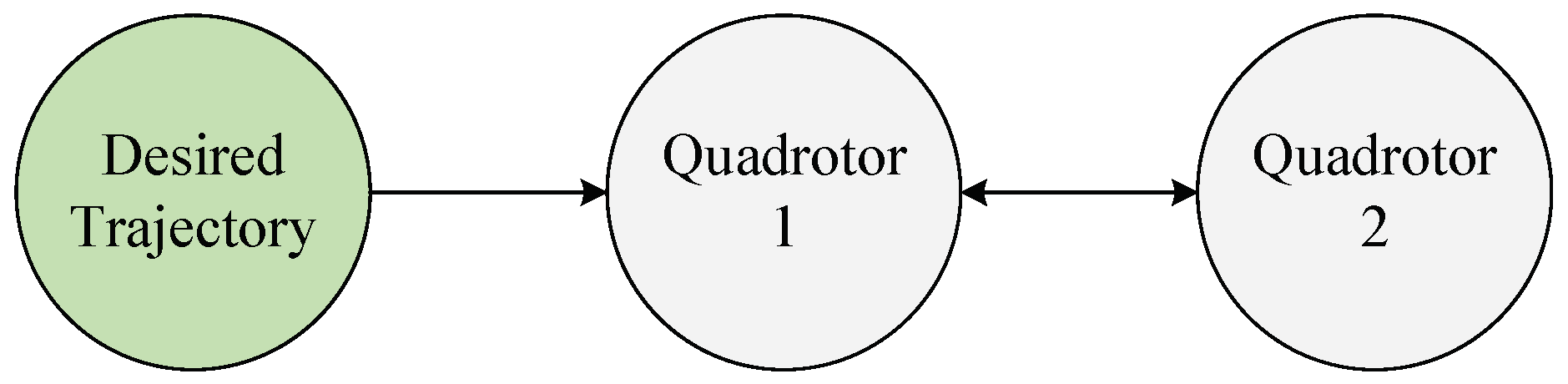
In this paper, the communication network topology among the quadrotors and the global reference system is described in Figure 4, where only Quadrotor 1 has access to the reference signals (desired trajectory ${\mathit{P}}_d^{\mathcal{I}}$ and desired formation yaw angle ${\delta }_d$), while the two quadrotors can exchange their own states, control inputs, and desired formation size $L_d$ via the network. In the rest of this paper, we generally use subscript “d” of a variable to denote its corresponding “desired” trajectory, i.e., its global reference signal.

Figure 4. The communication network topology.

The control objectives of this paper are to design a guidance law and robust cooperative controller for quadrotors under the communication network topology specified in Figure 4 such that the following are achieved:

(i)

The quadrotors achieve synchronized yaw angle tracking, i.e., ${\psi }_i\left(t\right)\to {\delta }_d\left(t\right)$ as $t\to \infty$;

(ii)

The quadrotors asymptotically track the desired trajectory in the desired, possibly time-varying formation specified by $L_d\left(t\right)$ in the absence of disturbances;

(iii)

In the presence of disturbances, the trajectory tracking error and the formation error can be quantitatively regulated within a small neighborhood of zero.

3. Guidance and Robust Control Design

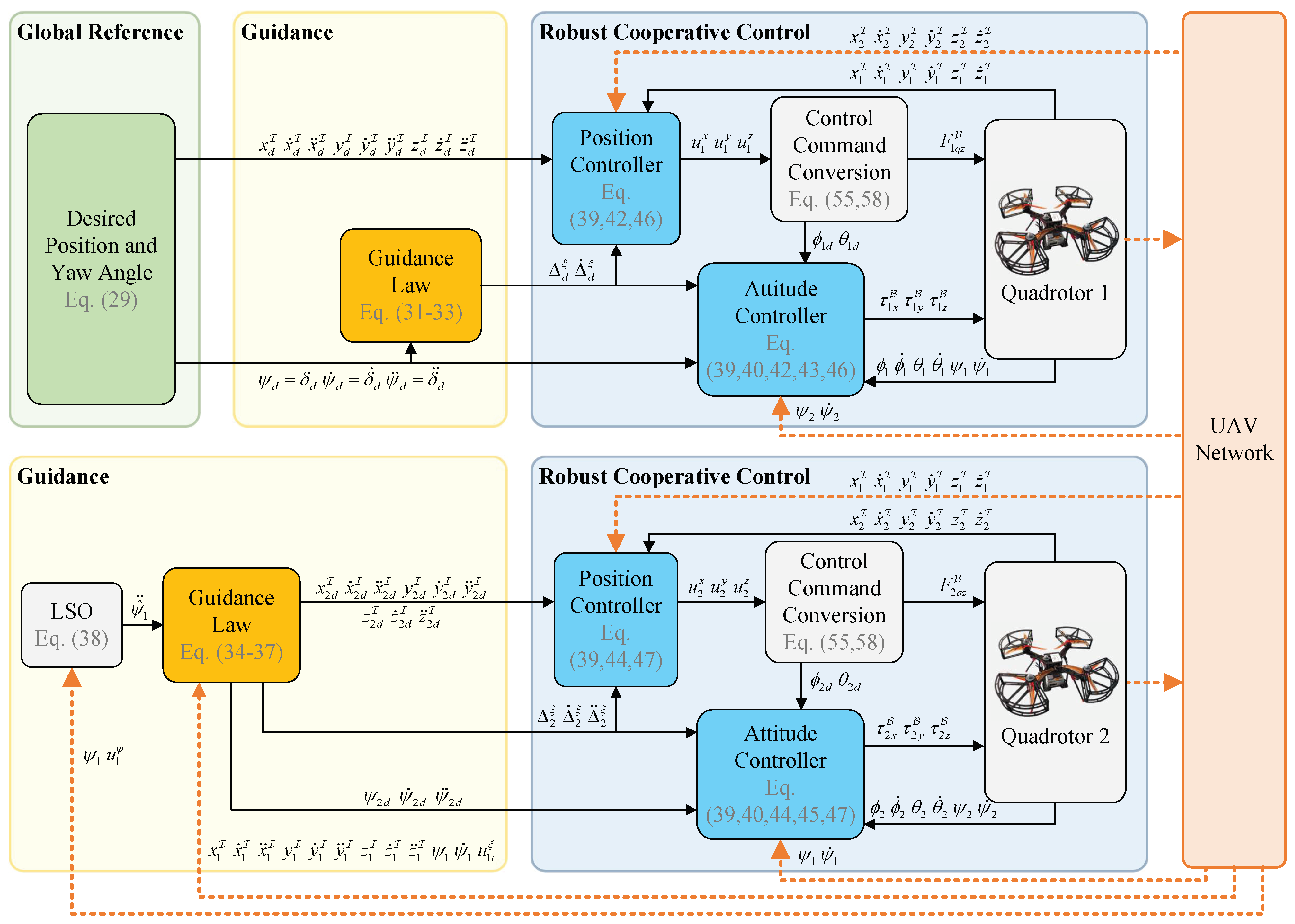
To achieve the aforementioned control objectives, we propose a novel two-module framework, as shown in Figure 5.

Figure 5. The proposed guidance and robust cooperative control scheme for the quadrotor formation.

Specifically, on the one hand, via the desired formation yaw angle ${\delta }_d$ and formation size $L_d$, one role of the guidance module is to generate the formation offset for the cooperative control module of the two quadrotors to achieve formation flight. Meanwhile, particularly for Quadrotor 2, another essential role is to calculate the local reference signals to address the unavailability of the global desired trajectory imposed by the communication topology specified in Figure 4.

On the other hand, the robust control module for each quadrotor includes a cooperative position controller, an attitude controller, and a control command conversion module that converts high-level acceleration commands into low-level attitude angle references and a thrust command $F_{iqz}^{\mathcal{B}}$. To deal with the disturbances induced by the payload swing, an uncertainty and disturbance estimator (UDE) that actively compensates for the disturbance is incorporated in both the position and attitude controllers.

In what follows, the design of each module is presented in detail.

3.1. Design of the Guidance Law

In this section, the global reference system is first defined, followed by the design of the guidance law for Quadrotor 2 to generate its local reference.

Suppose that the global desired trajectory for Quadrotor 1 satisfies

$${\ddot{\mathit{\xi }}}_{1d}={\mathit{u}}_{1d}^{\xi },$$

(29)

where ${\mathit{u}}_{1d}^{\xi }$ denotes the desired input. To form a formation with distance $L_d$ at yaw angle ${\delta }_d$, the desired trajectory for Quadrotor 2 is

$$\left\{\begin{array}{c}{\mathit{\xi }}_{2d}={\mathit{\xi }}_{1d}+{\mathbf{\Delta }}_d^{\xi },\hfill \\ {\dot{\mathit{\xi }}}_{2d}={\dot{\mathit{\xi }}}_{1d}+{\dot{\mathbf{\Delta }}}_d^{\xi },\hfill \\ {\ddot{\mathit{\xi }}}_{2d}={\mathit{u}}_{1d}^{\xi }+{\ddot{\mathbf{\Delta }}}_d^{\xi },\hfill \end{array}\right.$$

(30)

where ${\mathbf{\Delta }}_d^{\xi }$ represents the desired formation offset that satisfies

$${\mathbf{\Delta }}_d^{\xi }=\left[\begin{array}{c}{\mathsf{\Delta }}_d^{\psi }\\ {\mathsf{\Delta }}_d^x\\ {\mathsf{\Delta }}_d^y\\ {\mathsf{\Delta }}_d^z\end{array}\right]=\left[\begin{array}{c}0\\ L_{d}sin{\delta }_d\\ -L_{d}cos{\delta }_d\\ 0\end{array}\right].$$

(31)

The first-order and second-order derivatives of ${\mathbf{\Delta }}_d^{\xi }$ are

$${\dot{\mathbf{\Delta }}}_d^{\xi }=\left[\begin{array}{c}{\dot{\mathsf{\Delta }}}_d\\ {\dot{\mathsf{\Delta }}}_d^x\\ {\dot{\mathsf{\Delta }}}_d^y\\ {\dot{\mathsf{\Delta }}}_d^z\end{array}\right]=\left[\begin{array}{c}0\\ L_d{\dot{\delta }}_{d}cos{\delta }_d+{\dot{L}}_{d}sin{\delta }_d\\ L_d{\dot{\delta }}_{d}sin{\delta }_d-{\dot{L}}_{d}cos{\delta }_d\\ 0\end{array}\right]$$

(32)

and

$${\ddot{\mathbf{\Delta }}}_d^{\xi }=\left[\begin{array}{c}{\ddot{\mathsf{\Delta }}}_d^{\psi }\\ {\ddot{\mathsf{\Delta }}}_d^x\\ {\ddot{\mathsf{\Delta }}}_d^y\\ {\ddot{\mathsf{\Delta }}}_d^z\end{array}\right]=\left[\begin{array}{c}0\\ -L_d{\dot{\delta }}_d^{2}sin{\delta }_d+L_d{\ddot{\delta }}_{d}cos{\delta }_d+{\dot{L}}_d{\dot{\delta }}_{d}cos{\delta }_d+{\ddot{L}}_{d}sin{\delta }_d+{\dot{L}}_d{\dot{\delta }}_{d}cos{\delta }_d\\ L_d{\dot{\delta }}_d^{2}cos{\delta }_d+L_d{\ddot{\delta }}_{d}sin{\delta }_d+{\dot{L}}_d{\dot{\delta }}_{d}sin{\delta }_d-{\ddot{L}}_{d}cos{\delta }_d+{\dot{L}}_d{\dot{\delta }}_{d}sin{\delta }_d\\ 0\end{array}\right].$$

(33)

In this formation, the yaw angles and heights of the two quadrotors must be synchronized.

Note that for the $\psi$ channel in particular, we set ${\psi }_{id}={\delta }_d$ to ensure that the two quadrotors align their yaw angles with the formation yaw angle.

The desired trajectories (29) and (30) are called “global” reference systems, and they are specified by the prescribed control objectives. However, restricted by the communication topology, Quadrotor 2 does not have access to its global reference (30), and, thus, we are required to design Quadrotor 2’s guidance law to generate the “local” reference based on the neighboring information of Quadrotor 1 and the desired formation information $L_d$ such that the global objectives are achieved. The idea of this paper is to replace the unavailable desired signals in (30) with their corresponding states and the input of Quadrotor 1, which leads to the following guidance law (i.e., the local reference for Quadrotor 2):

$$\left\{\begin{array}{c}{\mathit{\xi }}_{2d}^{★}={\mathit{\xi }}_1+{\mathbf{\Delta }}_2^{\xi },\hfill \\ {\dot{\mathit{\xi }}}_{2d}^{★}={\dot{\mathit{\xi }}}_1+{\dot{\mathbf{\Delta }}}_2^{\xi },\hfill \\ {\ddot{\mathit{\xi }}}_{2d}^{★}={\mathit{u}}_{1t}^{\xi }+{\ddot{\mathbf{\Delta }}}_2^{\xi },\hfill \end{array}\right.$$

(34)

where ${\mathit{u}}_{1t}^{\xi }$ is the trajectory tracking control input term of Quadrotor 1 designed in Section 3.2, and formation offset ${\mathbf{\Delta }}_2^{\xi }$ uses ${\psi }_1$ to approximate ${\delta }_d$ and satisfies

$${\mathbf{\Delta }}_2^{\xi }=\left[\begin{array}{c}{\mathsf{\Delta }}_2^{\psi }\\ {\mathsf{\Delta }}_2^x\\ {\mathsf{\Delta }}_2^y\\ {\mathsf{\Delta }}_d^z\end{array}\right]=\left[\begin{array}{c}0\\ L_{d}sin{\psi }_1\\ -L_{d}cos{\psi }_1\\ 0\end{array}\right].$$

(35)

Then, ${\dot{\mathbf{\Delta }}}_2^{\xi }$ and ${\ddot{\mathbf{\Delta }}}_2^{\xi }$ are respectively given by

$${\dot{\mathbf{\Delta }}}_2^{\xi }=\left[\begin{array}{c}{\dot{\mathsf{\Delta }}}_2^{\psi }\\ {\dot{\mathsf{\Delta }}}_2^x\\ {\dot{\mathsf{\Delta }}}_2^y\\ {\dot{\mathsf{\Delta }}}_2^z\end{array}\right]=\left[\begin{array}{c}0\\ L_d{\dot{\psi }}_{1}cos{\psi }_1+{\dot{L}}_{d}sin{\psi }_1\\ L_d{\dot{\psi }}_{1}sin{\psi }_1-{\dot{L}}_{d}cos{\psi }_1\\ 0\end{array}\right]$$

(36)

and

$${\ddot{\mathbf{\Delta }}}_2^{\xi }=\left[\begin{array}{c}{\ddot{\mathsf{\Delta }}}_2^{\psi }\\ {\ddot{\mathsf{\Delta }}}_2^x\\ {\ddot{\mathsf{\Delta }}}_2^y\\ {\ddot{\mathsf{\Delta }}}_2^z\end{array}\right]=\left[\begin{array}{c}0\\ -L_d{\dot{\psi }}_1^{2}sin{\psi }_1+L_d{\ddot{\psi }}_{1}cos{\psi }_1+{\dot{L}}_d{\dot{\psi }}_{1}cos{\psi }_1+{\ddot{L}}_{d}sin{\psi }_1+{\dot{L}}_d{\dot{\psi }}_{1}cos{\psi }_1\\ L_d{\dot{\psi }}_1^{2}cos{\psi }_1+L_d{\ddot{\psi }}_{1}sin{\psi }_1+{\dot{L}}_d{\dot{\psi }}_{1}sin{\psi }_1-{\ddot{L}}_{d}cos{\psi }_1+{\dot{L}}_d{\dot{\psi }}_{1}sin{\psi }_1\\ 0\end{array}\right].$$

(37)

This guidance law design, however, causes another practical issue, that is, signal ${\ddot{\psi }}_1$ used in (37) is immeasurable. Therefore, we employ the following Luenberger state observer (LSO) to provide an estimate of ${\ddot{\psi }}_1$ denoted by ${\ddot{\hat{\psi }}}_1$:

$$\left[\begin{array}{c}{\dot{\hat{\psi }}}_1\\ {\ddot{\hat{\psi }}}_1\end{array}\right]=\left[\begin{array}{cc}-l_1& 1\\ -l_2& 0\end{array}\right]\left[\begin{array}{c}{\hat{\psi }}_1\\ {\dot{\hat{\psi }}}_1\end{array}\right]+\left[\begin{array}{c}{l}_1\\ l_2\end{array}\right]{\psi }_1+\left[\begin{array}{c}0\\ 1\end{array}\right]u_1^{\psi },$$

(38)

where ${\hat{\psi }}_1$ is the estimate of ${\psi }_1$; $l_1$ and $l_2$ are the observer feedback gains; and $u_1^{\psi }$ is the control input, which is designed in the following section.

3.2. Design of the Robust Controller

To achieve the control objectives, the controller should be designed to deliver the following: (i) the trajectory tracking of the global reference; (ii) the desired formation specified by $L_d$ and ${\delta }_d$; and (iii) payload swing disturbance rejection to ensure system robustness. Therefore, for the $\mathit{\xi }$ and $\mathit{\eta }$ channels, the robust controller is respectively designed as

$${\mathit{u}}_i^{\xi }={\mathit{u}}_{it}^{\xi }+{\mathit{u}}_{ic}^{\xi }-{\hat{\mathit{f}}}_i^{\xi },$$

(39)

$$\begin{array}{ccc}\hfill {\mathit{u}}_i^{\eta }& =& {\mathit{u}}_{it}^{\eta }-{\hat{\mathit{f}}}_i^{\eta },\hfill \end{array}$$

(40)

where ${\mathit{u}}_{it}^{\xi }$ and ${\mathit{u}}_{it}^{\eta }$ are the trajectory tracking terms, ${\mathit{u}}_{ic}^{\xi }$ is the cooperative control term that forms the desired formation, and ${\hat{\mathit{f}}}_i^{\xi }$ and ${\hat{\mathit{f}}}_i^{\eta }$ are the UDE terms (designed in Section 3.3) that compensate for the disturbances.

Remark 1. 

As shown in Figure 5, the reference system for the $\mathit{\xi }$ channel is given by an exogenous global reference (29) and a local reference (34) generated by the guidance law, whereas the $\mathit{\xi }$ channel, which represents the low-level tilt angle control system, obtains its reference signals based on the acceleration commands provided by the $\mathit{\xi }$ channel. Low-level reference signal generation is known as “control command conversion”, as detailed in Section 3.4.

Herein, we define the state tracking errors as

$$\left\{\begin{array}{c}{\tilde{\mathit{\xi }}}_i={\mathit{\xi }}_{id}-{\mathit{\xi }}_i,\hfill \\ {\tilde{\mathit{\eta }}}_i={\mathit{\eta }}_{id}-{\mathit{\eta }}_i.\hfill \end{array}\right.$$

(41)

Since Quadrotor 2 only has access to its local reference (34), we design a trajectory tracking controller for each quadrotor separately. For Quadrotor 1, the trajectory tracking terms are designed as

$$\begin{array}{ccc}\hfill {\mathit{u}}_{1t}^{\xi }& =& {\mathit{u}}_{1d}^{\xi }+k_{1p}^{\xi }{\tilde{\mathit{\xi }}}_1+k_{1d}^{\xi }{\dot{\tilde{\mathit{\xi }}}}_1,\hfill \end{array}$$

(42)

$$\begin{array}{ccc}\hfill {\mathit{u}}_{1t}^{\eta }& =& {\mathit{u}}_{1d}^{\eta }+k_{1p}^{\eta }{\tilde{\mathit{\eta }}}_1+k_{1d}^{\eta }{\dot{\tilde{\mathit{\eta }}}}_1,\hfill \end{array}$$

(43)

where ${\mathit{u}}_{1d}^{\xi }$ and ${\mathit{u}}_{1d}^{\eta }$ are the feedforward terms that drive the system move in a desired manner, $(k_{1p}^{\xi }{\tilde{\mathit{\xi }}}_1+k_{1d}^{\xi }{\dot{\tilde{\mathit{\xi }}}}_1)$ and $(k_{1p}^{\eta }{\tilde{\mathit{\eta }}}_1+k_{1d}^{\eta }{\dot{\tilde{\mathit{\eta }}}}_1)$ are the feedback terms that eliminate the trajectory tracking errors, and $k_{1p}^{\xi }$, $k_{1d}^{\xi }$, $k_{1p}^{\eta }$, and $k_{1d}^{\eta }$ are the feedback gains.

For Quadrotor 2, the trajectory tracking terms are designed as

$$\begin{array}{ccc}\hfill {\mathit{u}}_{2t}^{\xi }& =& {\ddot{\mathit{\xi }}}_{2d}^{★},\hfill \end{array}$$

(44)

$$\begin{array}{ccc}\hfill {\mathit{u}}_{2t}^{\eta }& =& {\mathit{u}}_{2d}^{\eta }+k_{2p}^{\eta }{\tilde{\mathit{\eta }}}_1+k_{2d}^{\eta }{\dot{\tilde{\mathit{\eta }}}}_2,\hfill \end{array}$$

(45)

where ${\ddot{\mathit{\xi }}}_{2d}^{★}$ is the feedforward control term provided by the local reference system (34).

To achieve cooperative formation control, we design the ${\mathit{u}}_{ic}^{\xi }$ term based on the formation offsets ${\mathbf{\Delta }}_d^{\xi }$ and ${\mathbf{\Delta }}_2^{\xi }$ given by (31) and (35), respectively. Therefore, we have

$$\begin{array}{ccc}\hfill {\mathit{u}}_{1c}^{\xi }& =& {\alpha }_1^{\xi }({\mathit{\xi }}_2-{\mathit{\xi }}_1-{\mathbf{\Delta }}_d^{\xi })+{\beta }_1^{\xi }({\dot{\mathit{\xi }}}_2-{\dot{\mathit{\xi }}}_1-{\dot{\mathbf{\Delta }}}_d^{\xi }),\hfill \end{array}$$

(46)

$$\begin{array}{ccc}\hfill {\mathit{u}}_{2c}^{\xi }& =& {\alpha }_2^{\xi }({\mathit{\xi }}_1-{\mathit{\xi }}_2+{\mathbf{\Delta }}_2^{\xi })+{\beta }_2^{\xi }({\dot{\mathit{\xi }}}_1-{\dot{\mathit{\xi }}}_2+{\dot{\mathbf{\Delta }}}_2^{\xi }),\hfill \end{array}$$

(47)

where ${\alpha }_i^{\xi }$ and ${\beta }_i^{\xi }$ are the position and velocity cooperative formation control gains.

Remark 2. 

In the design of the Quadrotor 2’s trajectory tracking control (44), we only include one feedforward term, as the feedback term, if designed based on the local reference system (34) as $k_{2p}^{\xi }({\mathit{\xi }}_{2d}^{★}-{\mathit{\xi }}_2)+k_{2d}^{\xi }({\dot{\mathit{\xi }}}_{2d}^{★}-{\dot{\mathit{\xi }}}_2)$, plays a similar role to the cooperative formation control term ${\mathit{u}}_{2c}^{\xi }$ given in (47). Therefore, the feedback term is omitted for Quadrotor 2.

3.3. Design of UDE

To enhance the robustness of the quadrotors against payload swing disturbance, the idea is to design an uncertainty and disturbance estimator (UDE) for each channel to dynamically estimate the disturbance in real time and then actively use the estimation signal to compensate for the disturbance. Since the models (28) for the $\mathit{\xi }$ and $\mathit{\eta }$ channels are in the same form, without the loss of generality, we first design the UDE for the $\mathit{\xi }$ channel, and then the results apply straightforwardly to the $\mathit{\eta }$ channel. Thus, the related discussion for the $\mathit{\eta }$ channel is omitted for simplicity.

Following the design principle of classic UDE-based control [17], we let the estimate of the disturbance, denoted by ${\hat{f}}_i^{\xi }$, satisfy the following relationship in the frequency domain by noting (28):

$${\hat{\mathit{F}}}_i^{\xi }\left(s\right)={\mathit{G}}_i^{\xi }\left(s\right){\mathit{F}}_i^{\xi }\left(s\right)={\mathit{G}}_i^{\xi }\left(s\right)[s^2{\mathit{\xi }}_i\left(s\right)-s{\mathit{\xi }}_i\left(0\right)-{\dot{\mathit{\xi }}}_i\left(0\right)-{\mathit{U}}_i^{\xi }\left(s\right)],$$

(48)

where we use the uppercase letter of a variable to denote its Laplace transform; ${\mathit{G}}_i^{\xi }\left(s\right)=diag\{G_i^{\psi }\left(s\right),G_i^x\left(s\right),G_i^y\left(s\right),G_i^z\left(s\right)\}$ is a transfer function matrix representing one design freedom of the UDE; and $G_i^{\xi }\left(s\right),\xi \in \{\psi ,x,y,z\}$ are strictly proper, stable, rational transfer functions to be designed later.

By assuming zero initial conditions and substituting (39) into (48), we obtain

$${\hat{\mathit{F}}}_i^{\xi }\left(s\right)={\mathit{G}}_i^{\xi }\left(s\right)[s^2{\mathit{\xi }}_i\left(s\right)-{\mathit{U}}_{it}^{\xi }\left(s\right)-{\mathit{U}}_{ic}^{\xi }\left(s\right)+{\hat{\mathit{F}}}_i^{\xi }\left(s\right)].$$

(49)

Solving ${\hat{\mathit{F}}}_i^{\xi }\left(s\right)$ from (49) yields

$${\hat{\mathit{F}}}_i^{\xi }\left(s\right)={[\mathit{I}-{\mathit{G}}_i^{\xi }\left(s\right)]}^{-1}{\mathit{G}}_i^{\xi }\left(s\right)[s^2{\mathit{\xi }}_i\left(s\right)-{\mathit{U}}_{it}^{\xi }\left(s\right)-{\mathit{U}}_{ic}^{\xi }\left(s\right)],$$

(50)

where $\mathit{I}$ is the identity matrix with compatible dimensions. The role of the transfer function $G_i^{\xi }\left(s\right)$ is to ensure the physical realizability of ${\hat{\mathit{F}}}_i^{\xi }\left(s\right)$, and, thus, we select

$$G_i^{\xi }\left(s\right)=\frac{1}{T_i^{\xi }s+1},\xi \in \{\psi ,x,y,z\},$$

(51)

where $T_i^{\xi }>0$ is the parameter that determines the UDE estimation bandwidth. Substituting (51) into (50) gives

$$\begin{array}{c}\hfill {\hat{\mathit{F}}}_i^{\xi }\left(s\right)={\mathit{T}}_i^{\xi }[s{\mathit{\xi }}_i\left(s\right)-\frac{1}{s}({\mathit{U}}_{it}^{\xi }\left(s\right)+{\mathit{U}}_{ic}^{\xi }\left(s\right))],\end{array}$$

(52)

where the gain matrix satisfies

$${\mathit{T}}_i^{\xi }=diag\{\frac{1}{T_i^{\psi }},\frac{1}{T_i^x},\frac{1}{T_i^y},\frac{1}{T_i^z}\}.$$

(53)

The time domain expression of (52) is

$${\hat{\mathit{f}}}_i^{\xi }\left(t\right)={\mathit{T}}_i^{\xi }[{\dot{\mathit{\xi }}}_i\left(t\right)-{\int }_0^t{\mathit{u}}_{it}^{\xi }\left(t\right)+{\mathit{u}}_{ic}^{\xi }\left(t\right)dt].$$

(54)

3.4. Control Command Conversion

In the classic quadrotor dual-loop control structure, the control command conversion module converts high-level commands into low-level references. For the $z_i$ channel, by using relationship (26), the thrust command $F_{iqz}$ is obtained as

$$F_{iqz}^{\mathcal{B}}=\frac{m(g-u_i^z)}{cos{\varphi }_{i}cos{\theta }_i}.$$

(55)

Moreover, the $x_i$ and $y_i$ channel control commands, representing the desired acceleration, are converted into the desired roll angle ${\varphi }_{id}$ and pitch angle ${\theta }_{id}$ given by

$$\begin{array}{ccc}\hfill {\theta }_{id}& =& arcsin(-\frac{m(u_i^{x}cos{\psi }_i+u_i^{y}sin{\psi }_i)}{F_{iqz}^{\mathcal{B}}cos{\varphi }_i}),\hfill \end{array}$$

(56)

$$\begin{array}{ccc}\hfill {\varphi }_{id}& =& arcsin(-\frac{m(u_i^{x}sin{\psi }_i-u_i^{y}cos{\psi }_i)}{F_{iqz}^{\mathcal{B}}}).\hfill \end{array}$$

(57)

To avoid the singularity issues encountered when $|\frac{m{u}_i^x}{F_{iqz}^{\mathcal{B}}cos{\varphi }_{i}cos{\psi }_i}|>1$ or $|\frac{m{u}_i^y}{F_{iqz}^{\mathcal{B}}cos{\psi }_i}|>1$, we apply the linear approximation $x\approx {sin}^{-1}\left(x\right)$ to (56) and (57) and obtain the reference signal for the $\mathit{\eta }$ channel:

$${\mathit{\eta }}_{id}=\left[\begin{array}{c}{\theta }_{id}\\ {\varphi }_{id}\end{array}\right]=\left[\begin{array}{c}-\frac{m(u_i^{x}cos{\psi }_i+u_i^{y}sin{\psi }_i)}{F_{iqz}^{\mathcal{B}}cos{\varphi }_i}\\ -\frac{m(u_i^{x}sin{\psi }_i-u_i^{y}cos{\psi }_i)}{F_{iqz}^{\mathcal{B}}}\end{array}\right].$$

(58)

Remark 3. 

The trajectory tracking control terms (43) and (45) require reference signal ${\dot{\mathit{\eta }}}_{id}$ and feedforward signal ${\mathit{u}}_{id}^{\eta }={\ddot{\mathit{\eta }}}_{id}$, which are the first- and second-order derivatives of ${\mathit{\eta }}_{id}$. In practical applications, if the quadrotors are not required to maneuver aggressively, these derivatives are insignificant and, thus, can be set to zero, which is implemented in most quadrotor flight control firmware. Otherwise, a numerical differentiation of ${\mathit{\eta }}_{id}$ might be needed.

3.5. Stability and Performance Analysis

In this section, the stability of the quadrotor formation and the robustness against disturbances are analyzed using singular perturbation theory. The conditions required for the feedback gains to ensure system stability are given in the following stability condition:

• Stability Condition 1. For the $\xi \in \{\psi ,x,y,z\}$ channels, $k_{ip}^{\xi }>0$, $k_{id}^{\xi }>0$, ${\alpha }_1^{\xi }+{\alpha }_2^{\xi }>0$, and ${\beta }_1^{\xi }+{\beta }_2^{\xi }>0$. For the $\eta \in \{\varphi ,\theta \}$ channels, $k_{ip}^{\eta }>0$, and $k_{id}^{\eta }>0$.

To simplify parameter tuning, we introduce the following parameter mapping:

$$\left\{\begin{array}{c}{T}_i^{\xi }=\epsilon T_i^{\xi *},\xi \in \{\psi ,x,y,z\},\hfill \\ T_i^{\eta }=\epsilon T_i^{\eta *},\eta \in \{\varphi ,\theta \},\hfill \end{array}\right.$$

(59)

where $\epsilon >0$ is the singular perturbation parameter that bridges the UDE parameters of the two quadrotors, and $T_i^{\xi *}$ and $T_i^{\eta *}$ are positive tunable parameters. Now, we are ready to present the main analysis results of the proposed guidance and control framework.

Theorem 1. 

Under Stability Condition 1, the following statements hold:

(i) 

All the states of the two quadrotors are bounded by applying the proposed guidance law and UDE-based robust controllers to the six channels;

(ii) 

The trajectory tracking errors of the quadrotor formation, as well as the low-level attitude angle tracking errors, can be quantitatively regulated and satisfy

$$\begin{array}{ccc}\hfill |{\tilde{\xi }}_i\left(t\right)|& \le & {\sigma }_i^{\xi }\left(\epsilon \right),\forall t>t_i^{\xi },\xi \in \{\psi ,x,y,z\},\hfill \end{array}$$

(60)

$$\begin{array}{ccc}\hfill |{\tilde{\eta }}_i\left(t\right)|& \le & {\sigma }_i^{\eta }\left(\epsilon \right),\forall t>t_i^{\eta },\eta \in \{\varphi ,\theta \},\hfill \end{array}$$

(61)

where ${\sigma }_i^{\xi }\left(\epsilon \right)$ and ${\sigma }_i^{\eta }\left(\epsilon \right)$ are the specified ultimate bounds of tracking errors ${\tilde{\xi }}_i\left(t\right)$ and ${\tilde{\eta }}_i\left(t\right)$, respectively, satisfying ${\sigma }_i^{\xi }\left(\epsilon \right)\to 0$ and ${\sigma }_i^{\eta }\left(\epsilon \right)\to 0$ as $\epsilon \to 0$, and $t_i^{\xi }$ and $t_i^{\eta }$ are their corresponding settling times.

Proof 

(Proof of Theorem 1). The proof of this theorem is presented in Appendix A. □

Remark 4. 

The statement (ii) of Theorem 1 shows that the system tracking performance and robustness are monotonic functions of ε; that is, by reducing a single parameter, ε, to enhance the disturbance rejection performance of the UDE, the quadrotor state tracking errors can be reduced to an arbitrarily small neighborhood of zero in the steady state. This feature is practically attractive because the parameter tuning for improving system robustness is simple and intuitive.

4. Simulation

In this section, the effectiveness of the proposed guidance and control framework for the two quadrotors carrying a suspended payload is verified numerically via MATLAB/Simulink simulations. Regarding the parameters and control gains used in the simulations, the parameters of the system are specified in Table 2, and the control gains are summarized in Table 3.

Table 3. Control gains used in the simulations.

Control Channels	Control Gains
	${\mathit{k}}_{\mathit{ip}}$	${\mathit{k}}_{\mathit{id}}$	${\alpha }_{\mathit{i}}$	${\beta }_{\mathit{i}}$	${\mathit{T}}_{\mathit{i}}^{*}$	$\epsilon$	${\mathit{l}}_{\mathbf{1}}$	${\mathit{l}}_{\mathbf{2}}$
x	3	2	5	5	1	1	\	\
y	3	2	5	5	1	1	\	\
z	$0.5$	1	5	5	$0.04$	1	\	\
$\varphi ,\theta$	20	20	\	\	$0.05$	1	\	\
$\psi$	3	2	5	5	1	1	100	100

The initial positions of the quadrotors are ${\mathit{P}}_1^{\mathcal{I}}\left(0\right)={[0m,0m,-1m]}^T$, ${\mathit{P}}_2^{\mathcal{I}}\left(0\right)={[0m,-1m,-1m]}^T$, and, thus, the initial formation size is $L\left(0\right)=1m$, while the initial formation yaw angle is $\delta \left(0\right)=0$ rad. The initial quadrotor attitude angles, the payload swing angles, and the quadrotor linear/angular velocities are all set to zero.

To show the capabilities of the proposed framework in terms of cooperative take-off, level flight, coordinated turn, formation size change, and formation flight manner change, we herein consider three different flight scenarios, as summarized in Table 4. Moreover, the system robustness against payload swing disturbance is verified in Scenario 4, where a set of different parameters $\epsilon =\{0.5,1,2,5\}$ is applied to the UDE during hovering. The simulation results for each scenario are detailed below.

Table 4. Scenarios considered in the simulations.

Scenario Number	Scenario Description
1	Take-off and level flight with varying formation size
2	Coordinated turn in a circular flight
3	Obstacle avoidance via time-varying formation flight
4	Robustness verification during hovering

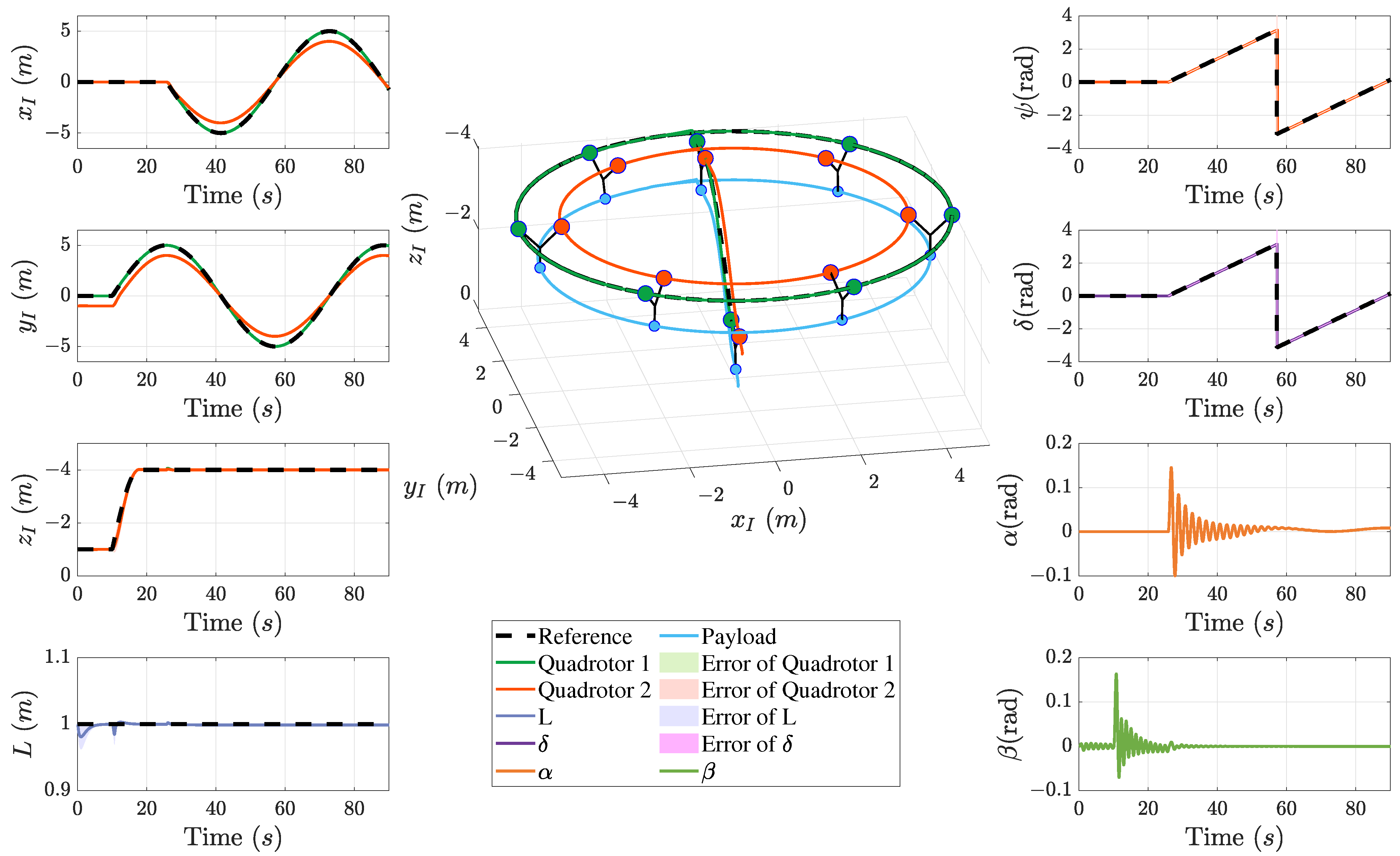
4.1. Scenario 1

In Scenario 1, the two quadrotors start by hovering at their initial positions for 10 s. Then, the two quadrotors carry the payload, ascend to an altitude of $z^{\mathcal{I}}=-4$ m, and fly along the $x^{\mathcal{I}}$-axis with a desired velocity of 0.1 m/s. For 40–60 s, the formation size L shrinks gradually from 1 m to 0.5 m at a constant speed and then maintains 0.5 m afterwards.

The simulation results are given in Figure 6 and Figure 7. From a stability and robustness viewpoint, it is seen that all system states are bounded during the flight, and robust trajectory tracking is achieved for the quadrotor formation under payload swing disturbance. Moreover, the proposed guidance law and cooperative controller enable the formation to change its size dynamically in a flight mission, and this capability is practically meaningful when the formation needs to pass through narrow corridors, as demonstrated in Scenario 3.

Figure 6. Scenario 1: flight trajectories of the formation and other states of the quadrotors and the payload.

Figure 7. Scenario 1: UDE disturbance estimation signals.

4.2. Scenario 2

Unlike Scenario 1, where the quadrotor formation flies forward along the $x_{{\mathcal{L}}_1}$-axis, i.e., where the flight direction is perpendicular to the two-quadrotor formation, Scenario 2 requires the quadrotor formation to fly laterally along the $y_{{\mathcal{L}}_1}$-axis to point ${\mathit{P}}_d^{\mathcal{I}}={[0m,5m,-1m]}^T$. Then, the quadrotor formation makes a coordinated turn in a circular flight path with a radius of 5 m by varying its yaw angle $\delta$. During the turn, the desired formation yaw angle ${\delta }_d$ increases at an angular velocity of 0.1 rad/s.

It is seen in Figure 8 that payload swing angle $\beta$ is stimulated by the lateral motion of the formation. But thanks to the disturbance estimation and rejection capability of the proposed UDE shown by Figure 9, the payload swing only causes a very small perturbation in the formation size L, as shown in Figure 8. Furthermore, in circular flight, the two quadrotors deliver excellent synchronized tracking performance of the desired formation yaw angle ${\delta }_d$, which results in high-accuracy trajectory tracking.

Figure 8. Scenario 2: flight trajectories of the formation and other states of the quadrotors and the payload.

Figure 9. Scenario 2: UDE disturbance estimation signals.

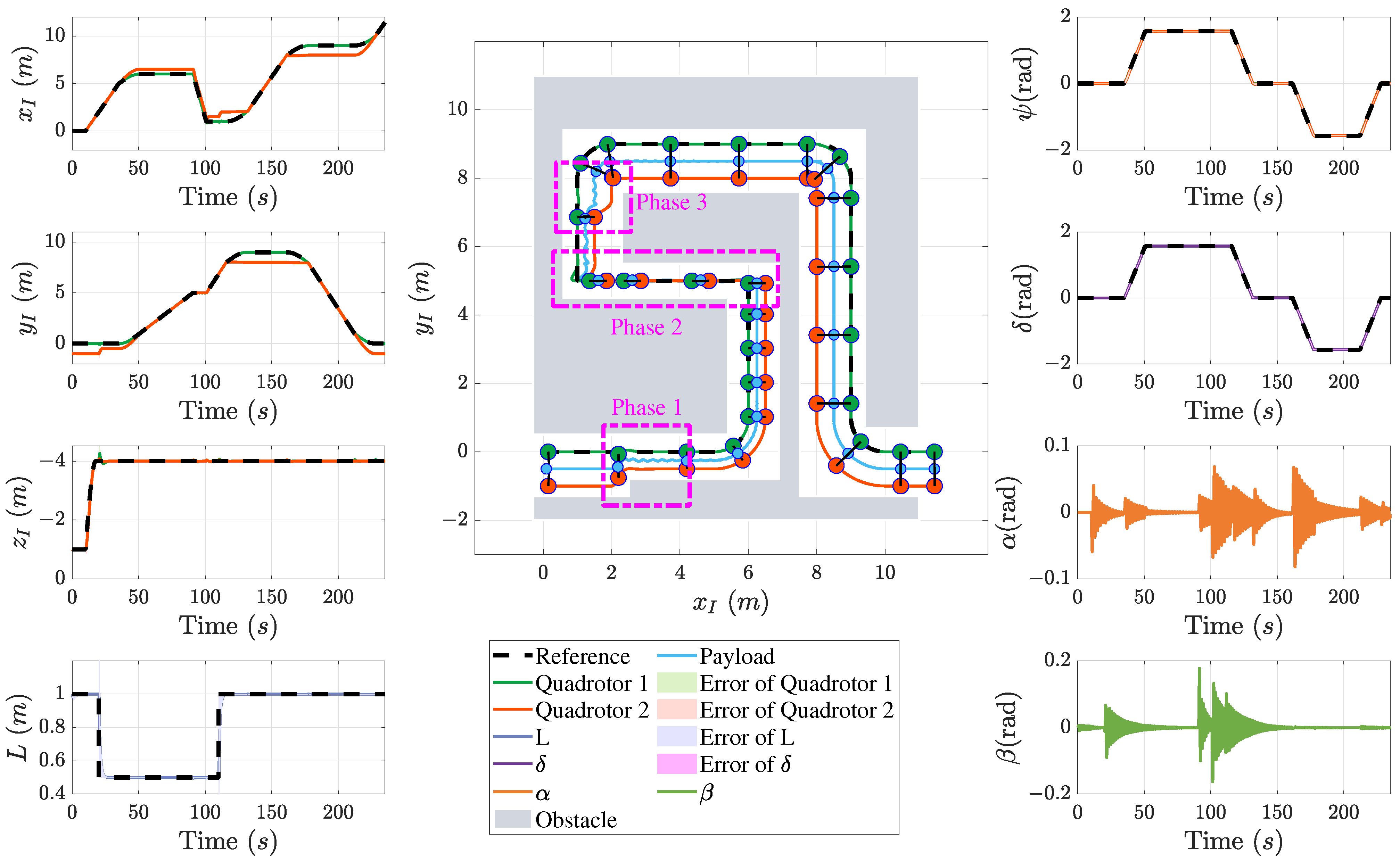
4.3. Scenario 3

The capability of the proposed methodology is best illustrated by its application in a complex flight environment, where the quadrotor formation passes through a narrow, winding corridor. The simulation results are given in Figure 10 and Figure 11. From Figure 10, it is observed that, to avoid collision, the formation size shrinks in Phase 1. When the corridor is too narrow to allow the quadrotor formation to fly through, as shown in Phase 2, the formation flies in a lateral manner instead and then restores its size in Phase 3 when the corridor becomes broader.

Figure 10. Scenario 3: flight trajectories of the formation and other states of the quadrotors and the payload.

Figure 11. Scenario 3: UDE disturbance estimation signals.

4.4. Scenario 4

To verify Theorem 1 presented in Section 3.5, that is, the notion that the tracking performance of the proposed control can be improved by decreasing a single parameter, $\epsilon$, we apply a set of $\epsilon =\{0.5,1,2,5\}$ to the UDE. Moreover, the proposed control without the UDE (denoted by “no compensation” in Figure 12) is also tested and compared to show the effectiveness of the UDE in terms of robustness enhancement. In this scenario, the quadrotors hover at their initial positions. The lateral component of the cable pulling force induced by the payload gravity on each quadrotor forces the quadrotors to become closer. It is seen in Figure 12 that, without the UDE to compensate for the disturbance force, the feedback control alone fails to maintain the formation size L. In contrast, when applying a smaller $\epsilon$ to the UDE, the deviation of the formation size becomes smaller. This result is consistent with the statement (ii) of Theorem 1, showing the advantage of the proposed control regarding parameter tuning.

Figure 12. Scenario 4: formation size and UDE disturbance estimation signals under different $\epsilon$ parameters.

5. Conclusions

This paper investigates the guidance and cooperative control of two quadrotors carrying a cable-suspended payload in a novel “Y”-shaped manner. To explicitly show the impact of payload swing on the linear motions of the two quadrotors, we first derive the payload swing motion dynamics associated with quadrotor acceleration, and then we establish a comprehensive, nonlinear, coupled quadrotor–payload model that converts the payload swing into disturbance cable pulling force vectors on the quadrotors. The comprehensive model is decoupled into six second-order subsystems by the feedback linearization technique. To address the problem of Quadrotor 2 not having access to the reference signals, a guidance law for Quadrotor 2 is proposed using Quadrotor 1’s measurable state information and estimates of unmeasurable state derivatives provided by a Luenberger state observer. Based on the local reference signals provided by the guidance law and the neighbor’s state information, uncertainty and disturbance estimator-based cooperative control is proposed for the two quadrotors to actively reject payload swing disturbance and achieve robust trajectory tracking in a desired, possibly time-varying formation. A singular perturbation theory-based performance analysis is provided, showing a practically attractive feature of the proposed control whereby the disturbance rejection performance and the overall trajectory tracking accuracy can be simultaneously improved by tuning one single parameter, $\epsilon$. Simulation results for three different scenarios are demonstrated to verify the effectiveness of the proposed control and its capability of achieving obstacle avoidance by varying the formation size and formation flight manner.

In the future, we aim to extend the proposed method to the cooperative formation control of multiple quadrotors carrying a suspended payload by cables in a “Y”-like shape. Specific steps include (1) deriving a generic model for the quadrotor–payload system and (2) designing a cooperative guidance law and local robust controller using multi-agent system distributed control theory.

References

- Liang, X.; Fang, Y.C.; Sun, N.; Lin, H. Nonlinear Hierarchical Control for Unmanned Quadrotor Transportation Systems. IEEE Trans. Ind. Electron. 2017, 65, 3395–3405. [Google Scholar] [CrossRef]
- Qian, L.H.; Graham, S.; Liu, H.H.T. Guidance and Control Law Design for a Slung Payload in Autonomous Landing: A Drone Delivery Case Study. IEEE ASME Trans. Mechatronics 2020, 25, 1773–1782. [Google Scholar] [CrossRef]
- Yang, S.; Xian, B. Energy-based Nonlinear Adaptive Control Design for the Quadrotor UAV System with a Suspended Payload. IEEE Trans. Ind. Electron. 2019, 67, 2054–2064. [Google Scholar] [CrossRef]
- Gimenez, J.; Gandolfo, D.C.; Salinas, L.R.; Rosales, C.; Carelli, R. Multi-objective Control for Cooperative Payload Transport with Rotorcraft UAVs. ISA Trans. 2018, 80, 491–502. [Google Scholar] [CrossRef] [PubMed]
- Liang, X.; Zhang, Z.; Yu, H.; Wang, Y.; Fang, Y.C.; Han, J.D. Antiswing Control for Aerial Transportation of the Suspended Cargo by Dual Quadrotor UAVs. IEEE/ASME Trans. Mechatronics 2022, 27, 5159–5172. [Google Scholar] [CrossRef]
- Alothman, Y.; Guo, M.H.; Gu, D.B. Using Iterative LQR to Control Two Quadrotors Transporting a Cable-suspended Load. IFAC-PapersOnLine 2017, 50, 4324–4329. [Google Scholar] [CrossRef]
- Villa, D.K.D.; Brandão, A.S.; Carelli, R.; Sarcinelli-Filho, M. Cooperative Load Transportation With Two Quadrotors Using Adaptive Control. IEEE Access 2021, 9, 129148–129160. [Google Scholar] [CrossRef]
- Pereira, P.O.; Dimarogonas, D.V. Nonlinear Pose Tracking Controller for Bar Tethered to Two Aerial Vehicles with Bounded Linear and Angular Accelerations. In Proceedings of the 2017 IEEE 56th Annual Conference on Decision and Control (CDC), Melbourne, Australia, 12–15 December 2017; pp. 4260–4265. [Google Scholar]
- Prajapati, P.; Parekh, S.; Vashista, V. Collaborative Transportation of Cable-Suspended Payload using Two Quadcopters with Human in the loop. In Proceedings of the 2019 28th IEEE International Conference on Robot and Human Interactive Communication (RO-MAN), New Delhi, India, 14–18 October 2019; pp. 1–6. [Google Scholar]
- Ccari, L.F.C.; Yanyachi, P.R. A Novel Neural Network-Based Robust Adaptive Formation Control for Cooperative Transport of a Payload Using Two Underactuated Quadcopters. IEEE Access 2023, 11, 36015–36028. [Google Scholar] [CrossRef]
- Aliyu, A.; El Ferik, S. Control of Multiple-UAV Conveying Slung Load With Obstacle Avoidance. IEEE Access 2022, 10, 62247–62257. [Google Scholar] [CrossRef]
- Chen, T.; Shan, J.J. Cooperative Transportation of Cable-suspended Slender Payload Using Two Quadrotors. In Proceedings of the 2019 IEEE International Conference on Unmanned Systems (ICUS), Beijing, China, 17–19 October 2019; pp. 432–437. [Google Scholar]
- Tang, S.; Sreenath, K.; Kumar, V. Aggressive Maneuvering of a Quadrotor with a Cable-Suspended Payload. In Proceedings of the Robotics: Science and Systems, Workshop on Women in Robotics, Berkeley, CA, USA, 12–16 July 2014; pp. 1–20. [Google Scholar]
- Chai, Y.; Liang, X.; Yang, Z.C.; Han, J.D. Energy-based Nonlinear Adaptive Control for Collaborative Transportation Systems. Aerosp. Sci. Technol. 2022, 126, 107510. [Google Scholar] [CrossRef]
- Lin, D.S.; Han, J.D.; Li, K.; Zhang, J.L.; Zhang, C.Y. Payload Transporting with Two Quadrotors by Centralized Reinforcement Learning Method. IEEE Trans. Aerosp. Electron. Syst. 2023, 60, 239–251. [Google Scholar] [CrossRef]
- Lu, Q.; Ren, B.B.; Parameswaran, S. Uncertainty and Disturbance Estimator-Based Global Trajectory Tracking Control for a Quadrotor. IEEE/ASME Trans. Mechatronics 2020, 25, 1519–1530. [Google Scholar] [CrossRef]
- Zhong, Q.C.; Rees, D. Control of Uncertain LTI Systems Based on an Uncertainty and Disturbance Estimator. J. Dyn. Sys. Meas. Control 2004, 126, 905–910. [Google Scholar] [CrossRef]
- Khalil, H.K.; Grizzle, J.W. Nonlinear Systems, 3rd ed.; Prentice-Hall: Upper Saddle River, NJ, USA, 2002; pp. 176–177. [Google Scholar]
Figure 1.
A comparison among the “V”-shaped [4,5,6], trapezoid-shaped [7,8,9], and proposed “Y”-shaped suspension method.
Figure 2.
Frames for the modeling.
Figure 3.
The forward–backward and lateral processes of the “Y”-shaped-cable-suspended payload swing motion.
Figure 4.
The communication network topology.
Figure 5.
The proposed guidance and robust cooperative control scheme for the quadrotor formation.
Figure 6.
Scenario 1: flight trajectories of the formation and other states of the quadrotors and the payload.
Figure 7.
Scenario 1: UDE disturbance estimation signals.
Figure 8.
Scenario 2: flight trajectories of the formation and other states of the quadrotors and the payload.
Figure 9.
Scenario 2: UDE disturbance estimation signals.
Figure 10.
Scenario 3: flight trajectories of the formation and other states of the quadrotors and the payload.
Figure 11.
Scenario 3: UDE disturbance estimation signals.
Figure 12.
Scenario 4: formation size and UDE disturbance estimation signals under different parameters.