Extended State Observer-Based Command-Filtered Safe Flight Control for Unmanned Helicopter under Time-Varying Path Constraints and Disturbances

Abstract

Unmanned helicopters are always subject to various external disturbances and constraints when performing tasks. In this paper, an extended state observer-based command-filtered safe tracking control scheme is investigated for an unmanned helicopter under time-varying path constraints and disturbances. To restrict the position states within the real-time safe flight boundaries, a safe reference path is regulated using the safe protection algorithm. The ESO is utilized to handle the unknown external disturbances. Moreover, the command filter technique is combined with the backstepping approach and twice inverse solution for the nonlinear unmanned helicopter system. According to the Lyapunov stability analysis, the safety and the tracking performance of the helicopter can be proved, and the availability of the safe tracking controller can also be illustrated by numerical simulations.

1. Introduction

In recent decades, the application of unmanned autonomous helicopters (UAH) in different fields has been rapidly promoted. Due to the universality and specific advantages of the UAH, more and more researchers focus on this area, and many studies have been carried out [1,2,3,4,5,6,7]. The authors used a multicriteria decision support method to model the unmanned helicopter in [1]. In [3], the authors introduced the nonlinear model of vario scale model helicopters and the establishment of a nonlinear control strategy. The authors in [4] combined the traditional backstepping method with the inner loop decoupling structure, which reduces the conservative design of the controller. In view of the inherent instability and strong nonlinear and coupling characteristics of small-scale UAHs, a nonlinear optimal control scheme was proposed in [6]. A special backstepping approach with inverse solution technique was investigated for a UAH system in [8], and has been widely adopted according to its flexible and effective controller design process. Furthermore, many characteristics, which are widely found in UAH, need to be considered, i.e., performance indexes, modeling uncertainties, and external disturbances.

Based on the fractional-order sliding mode control (SMC) method, the authors in [9] solved the external disturbances well. In addition, the extended state observer (ESO) was first proposed to compensate the uncertainties for nonlinear systems in [10]. Gradually, due to its strong approximation and lower dependence on plant information, the ESO-based control strategy was utilized widely to estimate not only the uncertainties [11,12] but also the unmeasured system states [13], external disturbances [7,14,15], and all sorts of combinations of the above [16,17]. In [7], by combining with the ESO, the SMC combined with a fault-tolerant control approach was developed for UAHs under wind disturbances. The authors proposed the fault-tolerant-based SMC scheme for the helicopter, and the ESO was used to solve the unknown wind gusts in [14]. In [18], the ESO technique was utilized for handling unmodeled disturbances for hydraulic system. However, the computing complexity will be increased dramatically by repeated differentiation.

To reduce the computing complexity, the command filter technique [19,20] was proposed. Due to the avoidance of differentiation and the satisfaction of estimation effect, command-filtered backstepping technologies are widely adopted in a number of control schemes [21,22,23,24,25]. In [26], based the backstepping technique, a finite-time command-filtered control scheme was adopted for quadcopter UAVs, and the problem of integration explosion was handled well. The command filtering technique was combined with the barrier Lyapunov function for the synchronous motor system in [27] Furthermore, besides the external disturbances, the UAH is usually subjected to state constraints when performing specific tasks, i.e., space prospecting in undetectable space [28], forest-fire monitoring [29], and so on.

During the flight process, the UAH system could suffer various path constraints because of the complex geography and specific mission requirements. How to guarantee the tracking performance of presupposed reference trajectory based on the safety requirements under path constraints needs to be further studied. The authors in [30] adopted the MPC method to accomplish the collision avoidance for the UAH. Employing the dynamic surface control (DSC) technique, the authors used a barrier Lyapunov function to prove the stability for an ammunition manipulator electrohydraulic system in [31]. Considering the prescribed performance, an adaptive fault-tolerant control scheme was investigated for a constrained UAH in [32].

Generally speaking, due to the changing environments and the special mission requirements, those path constraints are time-varying and cannot be predicted in advance in most situations. From a strategy of fixing desired trajectory, an obstacle avoidance method [33] was adopted in [34]. Similarly, the authors in [35] proposed a safe protection algorithm (SPA) to generate the safe desired signal for the unmanned helicopter.

This manuscript develops the SPA, which includes the predictive mechanism, to calculate a new safe reference trajectory within the real-time path constraints. A command-filtered backstepping method is utilized for tackling the problem of the piecewise differentiability of the constrained desired trajectory and the repeated derivation of the virtual control laws. Moreover, an ESO method is adopted to compensate unknown disturbances. The main contributions are illustrated as follows:

• A developed SPA with predictive characteristic is developed to obtain a new desired trajectory, which takes the time-varying path constraints into account. The path constraints violation can be detected earlier due to the predictive mechanism.
• The combination of the ESO and the command-filtered backstepping method is introduced to ensure that the generated safety trajectory is continuously differentiable, and the use of the command filter greatly reduces the computational complexity caused by the ESO.
• According to Lyapunov stability analysis, the signals of the UAH system are bounded, which means the UAH can track the presupposed desired trajectory on the basis of the safety requirement under path constraints and external disturbances.

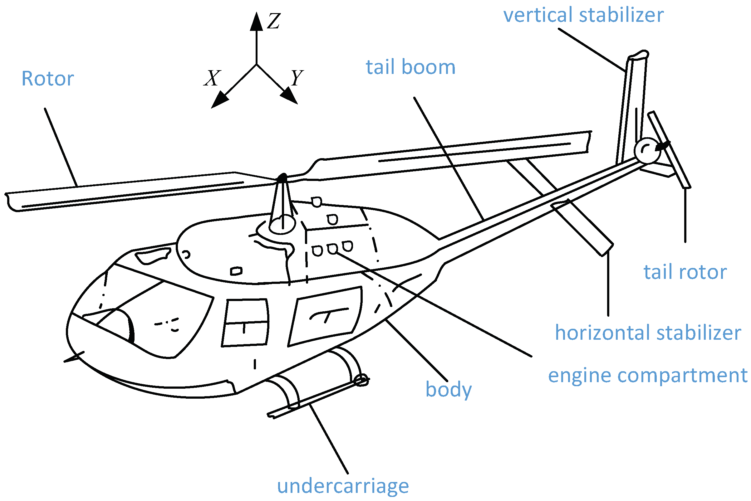
The remainder of this article consists of the following. In Section 2, the dynamics of the 14-state UAH and the problem formulation are detailed. In Section 3, the ESO-based command-filtered safe tracking control scheme is proposed. In Section 4, the performance of the proposed controller is verified by simulations. The conclusions are drawn in Section 5.

Notations: $I_n$ and $0_n$ represent the identity matrix and the zero matrix or vector with the dimension n, respectively. $f(·)$, $f^{\left(r\right)}(·)$ denotes its r-th-order time derivative. $A\succ 0$ denotes that A is a positive definite matrix.

2. Modeling and Problem Formulation

The UAH model is provided in Figure 1.

2.1. Modeling of the UAH System

The dynamics of the UAH under disturbances can be written as

$$\left\{\begin{array}{c}\dot{P}=v\hfill \\ m_0\dot{v}=R^{be}{F}_{mr}+G_0+d_v\hfill \\ \dot{\mathrm{\Omega }}=H\omega \hfill \\ J\dot{\omega }=-\omega \times J\omega +\mathrm{\Sigma }+d_{\mathrm{\Sigma }}\hfill \\ {\tau }_a\dot{a}=-{\tau }_{a}q-a+A_{lon}{T}_a+d_a\hfill \\ {\tau }_b\dot{b}=-{\tau }_{b}p-b+B_{lat}{T}_b+d_b\hfill \end{array}\right.$$

(1)

where $P={\left[X,Y,Z\right]}^{\mathrm{T}},v={\left[v_x,v_y,v_z\right]}^{\mathrm{T}},\mathrm{\Omega }={\left[\varphi ,\theta ,\psi \right]}^{\mathrm{T}},\omega ={\left[p,q,r\right]}^{\mathrm{T}}$ denote the positions of vector, velocity vector, attitude angle vector, and angular rate vector, respectively; $a,b\in \mathbb{R}$ denote the longitudinal flapping angle and lateral flapping angle of main rotor, respectively; $J=\mathrm{diag}\left\{J_{xx},J_{yy},J_{zz}\right\}$ represents the inertia matrix; $G_0={\left[0,0,m_0{g}_0\right]}^{\mathrm{T}}$ with the mass of UAH $m_0$ and gravity acceleration $g_0$; H and $R^{be}$ represent the attitude kinematic matrix and rotation matrix, respectively [4]; $A_{lon},B_{lat}$ denote steady-state gains; ${\tau }_a,{\tau }_b$ denote main rotor time constants; $T_a,T_b$ denote the longitudinal cyclic control and lateral cyclic control, respectively; $d_v,d_{\mathrm{\Sigma }}\in {\mathbb{R}}^3$ and $d_a,d_b\in \mathbb{R}$ represent unknown disturbances in the position subsystem, attitude subsystem, and rotor flapping subsystem, respectively; $F_{mr}={[0,0,-T_{mr}]}^{\mathrm{T}}$; $\mathrm{\Sigma }$ can be expressed as follows:

$$\mathrm{\Sigma }=\left[\begin{array}{c}{C}_{m}b+L_{mz}b{T}_{mr}-H_{mz}{T}_{tr}\\ C_{m}a+L_{mz}a{T}_{mr}\\ -\left(C_k{T}_{mr}^{1.5}+D_k\right)+H_{mx}{T}_{tr}\end{array}\right]$$

(2)

where $L_{mz},H_{mx},H_{mz}$ denote the distance vectors from the actuator to the center of ${\Re }_{body}$; $C_m,C_k,D_k$ denote the physical parameters of the main rotor, respectively. $Q_{mr}=C_k{T}_{mr}^{1.5}+D_k$.

In view of the underactuated characteristics of UAH, the dynamic system (1) is separated into the following three subsystems: the position subsystem ${\mathrm{\Psi }}_p$, attitude subsystem ${\mathrm{\Psi }}_a$, and rotor flapping subsystem ${\mathrm{\Psi }}_f$. For the convenience of controller design, the position subsystem ${\mathrm{\Psi }}_p$ is rewritten as

$${\mathrm{\Psi }}_p:\left\{\begin{array}{c}\dot{P}=v\hfill \\ \dot{v}=u/m_0+F_1+d_1\hfill \end{array}\right.$$

(3)

where $F_1={[0,0,g_0]}^{\mathrm{T}}$, $u=R^{be}{F}_{mr}$, and $d_1=d_v/m_0$. The attitude subsystem ${\mathrm{\Psi }}_a$ can be rewritten as

$${\mathrm{\Psi }}_a:\left\{\begin{array}{c}\dot{\mathrm{\Omega }}=H\omega \hfill \\ \dot{\omega }=F_2+J^{-1}\mathrm{\Sigma }+d_2\hfill \end{array}\right.$$

(4)

where $F_2=-J^{-1}\omega \times J\omega$ and $d_2=J^{-1}{d}_{\mathrm{\Sigma }}$. The rotor flapping subsystem ${\mathrm{\Psi }}_f$ can be rewritten as

$${\mathrm{\Psi }}_f:\dot{\chi }=F_3+G_{3}T+d_3$$

(5)

where

$$F_3=-\left[\begin{array}{c}q+a/{\tau }_a\\ p+b/{\tau }_b\end{array}\right],G_3=\left[\begin{array}{cc}{A}_{lon}/{\tau }_a& 0\\ 0& B_{lat}/{\tau }_b\end{array}\right],$$

$\chi ={[a,b]}^{\mathrm{T}}$, $T={[T_a,T_b]}^{\mathrm{T}}$, $d_3={[d_a/{\tau }_a,d_b/{\tau }_b]}^{\mathrm{T}}$.

2.2. Problem Formulation

Due to the universal geographical conditions during flight, it is important to consider the time-varying path constraints of UAH. Taking X as an example, $\forall t\ge 0$, define $X_{up}\left(t\right),X_{low}\left(t\right)\in \mathbb{R}$ as the upper and lower boundary of the constrained position state X, respectively. Similarly, another two position states Y and Z, also suffer from the time-varying path constraints $Y_{up}\left(t\right),Y_{low}\left(t\right)\in \mathbb{R}$ and $Z_{up}\left(t\right),Z_{low}\left(t\right)\in \mathbb{R}$. Thus, there exist time-varying position boundary vectors $P_{up}\left(t\right)={[X_{up}\left(t\right),Y_{up}\left(t\right),Z_{up}\left(t\right)]}^{\mathrm{T}}$ and $P_{low}\left(t\right)={[X_{low}\left(t\right),Y_{low}\left(t\right),Z_{low}\left(t\right)]}^{\mathrm{T}}$. Normally, defining $P_d$ is the desire signal. On this basis, the time-varying position boundaries $P_{up}$ and $P_{low}$ might conflict with $P_d$, which means that the assumed tracking performance does not apply to real-time flight.

The control objectives are given as follows:

(1)

To design an ESO-based command-filtered safe flight control scheme of the UAH system (1) with external disturbances.

(2)

To track the presupposed desired flight trajectory $P_d$ on the basis of satisfying the time-varying path constraints. If the path constraints conflict with $P_d$, the safety of the UAH turns into the first consideration.

Some assumptions are provided as follows:

Lemma 1

([20]). The command filter

$$\left\{\begin{array}{c}\dot{\lambda }=\mathrm{\Gamma }\eta \hfill \\ \dot{\eta }=-2\zeta \mathrm{\Gamma }\eta -\mathrm{\Gamma }(\lambda -h)\hfill \end{array}\right.$$

(6)

where $h,\lambda$ and η are the input, error, and auxiliary of the command filter, respectively. For all $t\ge 0$, if h satisfies $|\dot{h}|\le {\sigma }_1$ and $|\ddot{h}|\le {\sigma }_2$, where ${\sigma }_1,{\sigma }_2>0$, then for a positive constant δ, there exist $\mathrm{\Gamma }>0$ and $\zeta \in (0,1]$, that is $|\lambda -h|\le \kappa$, κ is a positive constant, $|\dot{\lambda }|$ and $|\ddot{\lambda }|$ are bounded.

Assumption A1

([9]). $\forall t\ge 0$, unknown time-varying disturbances $d_v\left(t\right),d_{\mathrm{\Sigma }}\left(t\right),d_a\left(t\right),d_b$ and there time derivatives are norm-bounded, which means the inequalities $\parallel {\dot{d}}_i\parallel \le {\xi }_i$ $(i=1,2,3,4)$ hold with unknown constants ${\xi }_i>0$.

Assumption A2

([4]). The states of UAH are measurable, and ϕ and θ are constrained from $-\pi /2$ to $\pi /2$.

Assumption A3

([9]). $\forall t\ge 0$, the desired trajectory $P_d$ and its time derivatives are norm bounded.

Assumption A4.

$\forall t\ge 0$, the safe boundaries $P_{up}\left(t\right)$, $P_{low}\left(t\right)$ and their first-order time derivatives ${\dot{P}}_{up}$, ${\dot{P}}_{low}$ and second-order time derivatives ${\ddot{P}}_{up}$, ${\ddot{P}}_{low}$ are norm-bounded, which means there exist known constants ${\xi }_{up}>0,{\xi }_{low}>0$ satisfies

$$\left\{\begin{array}{c}\begin{array}{c}{\Pi }_P^{up}=\left\{\left(P_{up},{\dot{P}}_{up},{\ddot{P}}_{up}\right):{∥P_{up}∥}^2+{\parallel {\dot{P}}_{up}\parallel }^2\right.\hfill \\ \left.+{\parallel {\ddot{P}}_{up}\parallel }^2\le {\xi }_{up}\right\}\hfill \end{array}\hfill \\ \begin{array}{c}{\Pi }_P^{low}=\left\{\left(P_{low},{\dot{P}}_{low},{\ddot{P}}_{low}\right):{∥P_{low}∥}^2+{\parallel {\dot{P}}_{low}\parallel }^2\right.\hfill \\ \left.+{\parallel {\ddot{P}}_{low}\parallel }^2\le {\xi }_{low}\right\}\hfill \end{array}\hfill \end{array}\right.$$

(7)

Remark 1.

The unmanned helicopter is equipped with various sensors, so it can sense the position and angular velocity information of the UAH in real time. The external disturbances are mainly caused by exogenous effects, and their energy is limited. Therefore, the external perturbations are always bounded.

3. ESO-Based Command-Filtered Safe Flight Control Scheme Design

In this section, an ESO-based command-filtered safe flight control scheme is investigated. As shown in Figure 2, the control system block diagram includes the following three parts: a safe reference trajectory design, an ESO-based command-filtered safe flight controller, and a 14-state UAH model.

3.1. Safe Reference Trajectory Design

Based on the reference path $P_d\left(t\right)$ under Assumption 3 and its smooth safe boundaries $P_{up}\left(t\right),P_{low}\left(t\right)$, a safe protection algorithm (SPA) is introduced in generating a safe reference path $P_s\left(t\right)$, which is strictly restricted in the time-varying position boundaries with the design margins.

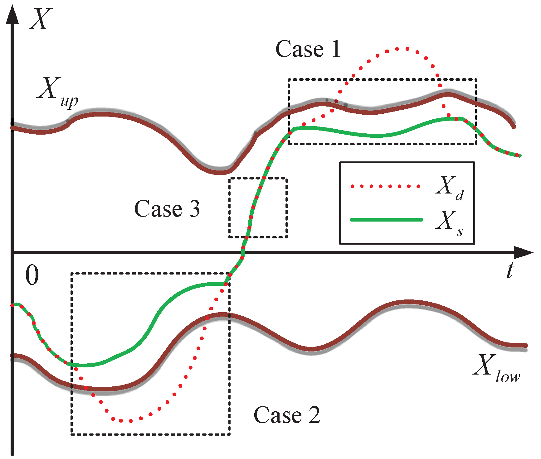
Without loss of generality, the position of the UAH in the X-axis is taken as an example and the generation of $X_s$ is illustrated in Figure 3, where the red dotted line is the original expected signal, the brown solid line is the safety boundary, and the green solid line is the safety expectation signal generated according to the original expected signal and the safety boundary. Define the time-varying margin in the following form:

$$b_x\left(t\right)=k_x\left[X_{up}\left(t\right)-X_{low}\left(t\right)\right]$$

(8)

where $k_x\in (0,0.5)$ denotes a design constant, whose choice is related to tracking performance and system safety.

In order to give the predictive property to the SPA, the real-time predicted time $T_x$ associated with $X_d$, $X_{up}$, and $X_{low}$ is expressed by

$$T_x={\displaystyle \frac{b_x}{4{\Delta }_x+b_x/{\overline{T}}_x}}$$

(9)

where

$${\Delta }_x\left(t\right)=\underset{\rho \in [t,t+\Delta {\overline{t}}_c]}{max}\left(|{\dot{X}}_{\overline{p}}\left(\rho \right)|\right)\ge 0$$

(10)

where $\overline{p}$ stands for $d,up,low,$ $\Delta {\overline{t}}_c>0$ is the maximum predict time to be designed. Combining (11) with (10), one can obtain that the following equation:

$$T_x\le {\displaystyle \frac{b_x}{b_x/{\overline{\Delta }}_x}}={\overline{T}}_x,\forall t\ge 0$$

(11)

always holds; namely, ${\overline{T}}_x$ is the maximum of time-varying predicted time $T_x$.

Different from $X_d(t+T_x)$, the values of $X_{up}(t+T_x)$ and $X_{low}(t+T_x)$ at time t cannot be obtained directly; the related estimation needs to be introduced. By assuming that $X_{\ell }$ ($\ell \in \{up,low\}$) evolves by a constant rate, the predictive value at time $t+T_x$ is given as

$${\widehat{X}}_{\ell }(t+T_x)=X_{\ell }+{\dot{X}}_{\ell }·T_x,$$

(12)

where ${\dot{X}}_{\ell }$ is the time derivative of $X_{\ell }$ by the first-order differentiator [9].

For written convenience, $\forall t\ge 0$, define

$$\left\{\begin{array}{c}\Delta x_{\ell }={\widehat{X}}_{\ell }(t+T_x)-X_{\ell }\\ \Delta x_d=X_d(t+T_x)-X_d.\end{array}\right.$$

(13)

where $\ell \in \{up,low\}$. Accordingly, the real-time safety margins ${\mu }_{x,up}$, ${\mu }_{x,low}$ are calculated by

$$\left\{\begin{array}{c}{\mu }_{x,up}=b_x-\Delta x_{up}+\Delta x_d\hfill \\ {\mu }_{x,low}=b_x+\Delta x_{low}-\Delta x_d.\hfill \end{array}\right.$$

(14)

Remark 2.

$b_x$ is constrained within $(0,0.5)$, which can ensure that the conditions of Case I and II in Figure 3 cannot be satisfied simultaneously.

In order to add the predictive mechanism of SPA, the path constraints violation at time $t+T_x$ should be discussed; $X_s$ and its derivatives $X_s^{\left(r\right)}\left(t\right)$$(r=0,1,2)$ can be calculated by following three cases:

• Case I: At time t, the presupposed desired trajectory $X_d(t+T_x)$ will be greater than the predicted upper path constraint $X_{up}(t+T_x)$ with ${\rho }_x$.

To keep the safe reference trajectory $X_s$ within upper path constraint $X_{up}$, $X_s^{\left(r\right)}$ is calculated by

$$X_s^{\left(r\right)}=X_{up}^{\left(r\right)}-{\mu }_{x,up}^{\left(r\right)}.$$

(15)

• Case II: At time t, the presupposed desired trajectory $X_d(t+T_x)$ will be less than the predicted lower path constraint $X_{up}(t+T)$ with ${\rho }_x$.

To keep the safe reference trajectory $X_s$ within lower path constraint $X_{low}$, $X_s^{\left(r\right)}$ is calculated by

$$X_s^{\left(r\right)}=x_{low}^{\left(r\right)}\left(t\right)+{\mu }_{x,low}^{\left(r\right)}.$$

(16)

• Case III: The UAH is expected to track the presupposed reference path $X_d$.

In other words, $X_s^{\left(r\right)}$ is calculated by

$$X_s^{\left(r\right)}=X_d^{\left(r\right)}.$$

(17)

The judgment of the violation can be illustrated in Figure 4, and the calculation of the real-time safety margins ${\mu }_{x,up}\left(t\right)$, ${\mu }_{x,low}\left(t\right)$ in (14) have been shown intuitively in Figure 5. In Figure 5, the red dashed line is the original expected signal, the orange solid line is the safety boundary, and the green solid line is the generated safety expected signal. Invoking (15)–(17), the safe reference path $X_s$ can be obtained as follows:

$$X_s^{\left(r\right)}\left(t\right)=\left\{\begin{array}{cc}{X}_{up}^{\left(r\right)}\left(t\right)-{\mu }_{x,up}^{\left(r\right)}\left(t\right),\hfill & \mathrm{if}\mathrm{Case}1\\ X_{low}^{\left(r\right)}\left(t\right)+{\mu }_{x,low}^{\left(r\right)}\left(t\right),\hfill & \mathrm{if}\mathrm{Case}2\\ X_d^{\left(r\right)}\left(t\right)\hfill & \mathrm{if}\mathrm{Case}3\end{array}\right.$$

(18)

The boundedness of $X_s$ can be proved as the following theorem.

Theorem 1.

$\forall t\ge 0$, if $X_d\left(0\right)\in [X_{low}\left(0\right),X_{up}\left(0\right)]$, the safe reference trajectory $X_s\left(t\right)$ can be constrained in the real-time interval $[X_{low}\left(t\right),X_{up}\left(t\right)]$ under a design minimum margin ${\underline{\mu }}_x$ satisfying

$${\underline{\mu }}_x=k_x\underset{t\ge 0}{min}{\displaystyle \frac{X_{up}\left(t\right)-X_{low}\left(t\right)}{2}}$$

(19)

Proof of Theorem 1.

In light of (8)–(13), $\forall t\ge 0$, we can obtain that

$$\begin{array}{c}\left|\Delta x_{\ell }\left(t\right)\right|\le {\Delta }_x\left(t\right)·\underset{\tau \in [t,t+{\Delta }_x\left(t\right)]}{max}\left|{\dot{x}}_{\ell }\left(\tau \right)\right|\hfill \\ \le {\displaystyle \frac{b_x\left(t\right)}{4{\Delta }_x\left(t\right)}}·\underset{\tau \in [t,t+{\overline{\Delta }}_x]}{max}\left|{\dot{x}}_{\ell }\left(\tau \right)\right|={\displaystyle \frac{b_x\left(t\right)}{4}}\hfill \end{array}$$

(20)

with $\ell \in \{d,up,low\}$.

It follows from (10), (14), (19), and (20) that

$$\begin{array}{c}{\mu }_{x,\ell }\left(t\right)\ge b_x\left(t\right)-\left|\Delta x_d\left(t\right)\right|-\left|\Delta x_{\ell }\left(t\right)\right|\hfill \\ \ge {\displaystyle \frac{1}{2}}{b}_x\left(t\right)\ge {\underline{\mu }}_x,\forall t\ge 0.\hfill \end{array}$$

(21)

with $\ell \in \{up,low\}$.

Considering (18), we can obtain that if $X_d\left(0\right)\in (X_{low}\left(0\right),X_{up}\left(0\right))$, $X_s\left(t\right)$ can be guaranteed in the interval $(X_{low}\left(t\right),X_{up}\left(t\right))$ for all $t\ge 0$ with a design minimum margin ${\underline{\mu }}_x$.

This concludes the proof. □

It follows from Theorem 1 that the safe reference path $X_s$ can be restricted in the safe boundaries $X_{up}\left(t\right)$ and $X_{low}\left(t\right)$ with a safety margin ${\underline{\mu }}_x$. Moreover, the same process can be designed for Y and Z. Thus, the safe reference paths $Y_s$, $Z_s$ and their time derivatives ${\dot{Y}}_s$, ${\dot{Z}}_s$, ${\ddot{Y}}_s$ and ${\ddot{Z}}_s$ can also be calculated with the safety margins ${\underline{\mu }}_y$, ${\underline{\mu }}_z$ by designing the design constants $k_y\in (0,0.5)$, $k_z\in (0,0.5)$.

In accordance with Assumptions 3 and 4, Theorem 1, and (18), we can obtain that ${\mathrm{{\rm Y}}}_s^{\left(r\right)}\left(t\right)$ $(\mathrm{{\rm Y}}\in \{X,Y,Z\},r=0,1,2)$ is bounded. Namely,

$$∥{\mathrm{{\rm Y}}}_s^{\left(r\right)}\left(t\right)∥\le {\xi }_{\mathrm{{\rm Y}},r},\mathrm{{\rm Y}}\in \{X,Y,Z\},r=0,1,2,$$

(22)

where ${\xi }_{\mathrm{{\rm Y}},r}$ represents a positive constraint.

3.2. Design of the Command Filters

In order to handle the safe reference path $P_s={[X_s,Y_s,Z_s]}^{\mathtt{T}}$ and the virtual control signals $v_d$, ${\mathrm{\Omega }}_d$, ${\omega }_d$, and ${\chi }_d$ to be designed later, the command filter technology is introduced.

Firstly, the tracking error vectors are designed as

$$\begin{array}{c}{z}_1=P-{\lambda }_P,z_2=v-{\lambda }_v,\hfill \\ z_3=\mathrm{\Omega }-{\lambda }_{\mathrm{\Omega }},z_4=\omega -{\lambda }_{\omega },\hfill \\ z_5=\chi -{\lambda }_{\chi },\hfill \end{array}$$

(23)

and the error compensations for command filter as

$$e_i=z_i-{\gamma }_i,1\le i\le 5$$

(24)

where ${\lambda }_P$, ${\lambda }_v$, ${\lambda }_{\mathrm{\Omega }}$, ${\lambda }_{\omega }$, ${\lambda }_{\chi }$ denote the outputs of the command filters with $P_s$, $v_d$, ${\mathrm{\Omega }}_s$, ${\omega }_d$, ${\chi }_s$ being the inputs and ${\gamma }_i$ being the compensating signals.

For the safe reference path $P_s$, the command filter is constructed as

$$\left\{\begin{array}{c}{\dot{\lambda }}_P={\mathrm{\Gamma }}_P{\eta }_P\hfill \\ {\dot{\eta }}_P=-2{\zeta }_P{\mathrm{\Gamma }}_P{\eta }_P-{\mathrm{\Gamma }}_P({\lambda }_P-P_s)\hfill \end{array}\right.$$

(25)

where ${\eta }_P\in {\mathbb{R}}^3$ denotes the auxiliary variable of the command filter, ${\mathrm{\Gamma }}_P\in {\mathbb{R}}^{3\times 3}$ represents a design matrix and ${\zeta }_P\in (0,1]$ is a design constant. In addition, ${\lambda }_P\left(0\right)=P_s\left(0\right)$ and ${\eta }_P\left(0\right)=0_3.$

$v_d$, ${\mathrm{\Omega }}_d$, ${\omega }_d$, and ${\chi }_d$ are the virtual control signals. To reduce computational complexity, the command filters are designed as

$$\left\{\begin{array}{c}{\dot{\lambda }}_v={\mathrm{\Gamma }}_v{\eta }_v\hfill \\ {\dot{\eta }}_v=-2{\zeta }_v{\mathrm{\Gamma }}_v{\eta }_v-{\mathrm{\Gamma }}_v({\lambda }_v-v_d)\hfill \end{array}\right.$$

(26)

$$\left\{\begin{array}{c}{\dot{\lambda }}_{\mathrm{\Omega }}={\mathrm{\Gamma }}_{\mathrm{\Omega }}{\eta }_{\mathrm{\Omega }}\hfill \\ {\dot{\eta }}_{\mathrm{\Omega }}=-2{\zeta }_{\mathrm{\Omega }}{\mathrm{\Gamma }}_{\mathrm{\Omega }}{\eta }_{\mathrm{\Omega }}-{\mathrm{\Gamma }}_{\mathrm{\Omega }}({\lambda }_{\mathrm{\Omega }}-{\mathrm{\Omega }}_d)\hfill \end{array}\right.$$

(27)

$$\left\{\begin{array}{c}{\dot{\lambda }}_{\omega }={\mathrm{\Gamma }}_{\omega }{\eta }_{\omega }\hfill \\ {\dot{\eta }}_{\omega }=-2{\zeta }_{\omega }{\mathrm{\Gamma }}_{\omega }{\eta }_{\omega }-{\mathrm{\Gamma }}_{\omega }({\lambda }_{\omega }-{\omega }_d)\hfill \end{array}\right.$$

(28)

and

$$\left\{\begin{array}{c}{\dot{\lambda }}_{\chi }={\mathrm{\Gamma }}_{\chi }{\eta }_{\chi }\hfill \\ {\dot{\eta }}_{\chi }=-2{\zeta }_{\chi }{\mathrm{\Gamma }}_{\chi }{\eta }_{\chi }-{\mathrm{\Gamma }}_{\chi }({\lambda }_{\chi }-{\chi }_d)\hfill \end{array}\right.$$

(29)

where ${\eta }_v,{\eta }_{\mathrm{\Omega }},{\eta }_{\omega }\in {\mathbb{R}}^3$, and ${\eta }_{\chi }\in {\mathbb{R}}^2$ denote auxiliary variables; ${\mathrm{\Gamma }}_v,{\mathrm{\Gamma }}_{\mathrm{\Omega }},{\mathrm{\Gamma }}_{\omega }\in {\mathbb{R}}^{3\times 3}$, and ${\mathrm{\Gamma }}_{\chi }\in {\mathbb{R}}^{2\times 2}$ denote the design diagonal positive definite matrices, design constants; and ${\zeta }_v,{\zeta }_{\mathrm{\Omega }},{\zeta }_{\omega },{\zeta }_{\chi }\in (0,1]$ are constants to be designed. ${\lambda }_v\left(0\right)=v_d\left(0\right)$, ${\lambda }_{\mathrm{\Omega }}\left(0\right)={\mathrm{\Omega }}_d\left(0\right)$, ${\lambda }_{\omega }\left(0\right)={\omega }_d\left(0\right)$, ${\lambda }_{\chi }\left(0\right)={\chi }_d\left(0\right)$, ${\eta }_v\left(0\right)={\eta }_{\mathrm{\Omega }}\left(0\right)={\eta }_{\omega }\left(0\right)=0_3$, ${\eta }_{\chi }\left(0\right)=0_2$.

For removing the effect of the errors between the outputs and inputs of designed command filters, the compensating signals are designed as

$$\left\{\begin{array}{c}{\dot{\gamma }}_1=-K_{\gamma 1}{\gamma }_1+{\gamma }_2+\left({\lambda }_v-v_d\right)\hfill \\ {\dot{\gamma }}_2=-K_{\gamma 2}{\gamma }_2\hfill \\ {\dot{\gamma }}_3=-K_{\gamma 3}{\gamma }_3+H{\gamma }_4+H\left({\lambda }_{\omega }-{\omega }_d\right)\hfill \\ {\dot{\gamma }}_4=-K_{\gamma 4}{\gamma }_4\hfill \\ {\dot{\gamma }}_5=-K_{\gamma 5}{\gamma }_5,\hfill \end{array}\right.$$

(30)

where $K_{\gamma i}$ denotes the positive definite matrices with compatible dimensions to be designed and ${\gamma }_i\left(0\right)=0_3$, (i=1,2, 3, 4), ${\gamma }_5\left(0\right)=0_2$.

According to Lemma 1, the tracking errors of the designed command filters (25)–(29) can be converged to an arbitrary small field by choosing appropriate parameters. Namely, by choosing ${\mathrm{\Gamma }}_P$, ${\mathrm{\Gamma }}_v$, ${\mathrm{\Gamma }}_{\mathrm{\Omega }}$, ${\mathrm{\Gamma }}_{\omega }$, ${\mathrm{\Gamma }}_{\chi }$, ${\zeta }_P$, ${\zeta }_v$, ${\zeta }_{\mathrm{\Omega }}$, ${\zeta }_{\omega }$, and ${\zeta }_{\chi }$, one has

$$\begin{array}{c}∥{\lambda }_P-P_s∥\le {\kappa }_P,∥{\lambda }_v-v_d∥\le {\kappa }_v,\hfill \\ ∥{\lambda }_{\mathrm{\Omega }}-{\mathrm{\Omega }}_s∥\le {\kappa }_{\mathrm{\Omega }},∥{\lambda }_{\omega }-{\omega }_d∥\le {\kappa }_{\omega },\hfill \\ ∥{\lambda }_{\chi }-{\chi }_d∥\le {\kappa }_{\chi },\hfill \end{array}$$

where ${\kappa }_P,{\kappa }_v,{\kappa }_{\mathrm{\Omega }},{\kappa }_{\omega },{\kappa }_{\chi }$ are positive constants.

Furthermore, $∥{\gamma }_i∥$ is bounded, which holds [20]

$$∥{\gamma }_i∥\le {\xi }_{\gamma }=\sqrt{{\displaystyle \frac{{\kappa }^2}{2k_0}}},i=1,\dots ,5$$

(31)

where

$$\left\{\begin{array}{c}\kappa ={\kappa }_P+{\kappa }_v+{\kappa }_{\mathrm{\Omega }}+{\kappa }_{\omega }+{\kappa }_{\chi }\hfill \\ k_0=min\left\{\begin{array}{c}{\lambda }_{min}\left(K_{\gamma 1}-I_3\right),{\lambda }_{min}\left(K_{\gamma 2}-I_3\right),\hfill \\ {\lambda }_{min}\left(K_{\gamma 3}-I_3\right),{\lambda }_{min}\left(K_{\gamma 4}-I_3\right),\hfill \\ {\lambda }_{min}\left(K_{\gamma 5}-I_2\right)\hfill \end{array}\right\}.\hfill \end{array}\right.$$

3.3. ESO-Based Command-Filtered Safe Flight Controller Design in Position Subsystem

Considering (3) and (24), we have

$$\begin{array}{c}{\dot{e}}_1={\dot{z}}_1-{\dot{\gamma }}_1=\left(\dot{P}-{\dot{\lambda }}_P\right)-{\dot{\gamma }}_1\hfill \\ =\left(e_2+{\gamma }_2+{\lambda }_v-{\dot{\lambda }}_P\right)-\left[-K_{\gamma 1}{\gamma }_1+{\gamma }_2+\left({\lambda }_v-v_d\right)\right]\hfill \\ =e_2+K_{\gamma 1}{\gamma }_1-{\dot{\lambda }}_P+v_d.\hfill \end{array}$$

(32)

The virtual controller is given by

$$v_d=-K_1{e}_1-K_{\gamma 1}{\gamma }_1+{\dot{\lambda }}_P,$$

(33)

where $K_1=K_1^{\mathtt{T}}\succ 0$ is a matrix with compatible dimensions to be designed. Substituting (33) to (32) yields

$${\dot{e}}_1=-K_1{e}_1+e_2.$$

(34)

Differentiating $e_2$ yields

$$\begin{array}{cc}\hfill {\dot{e}}_2& ={\dot{z}}_2-{\dot{\gamma }}_2\hfill \\ \hfill & =\left(\dot{v}-{\dot{\lambda }}_v\right)-{\dot{\gamma }}_2\hfill \\ \hfill & =\left(u/m_0+F_1+d_1-{\dot{\lambda }}_v\right)+K_{\gamma 2}{\gamma }_2.\hfill \end{array}$$

(35)

Considering (3), to estimate the unknown disturbance, an ESO is introduced. Defining $x_{d1}$ is the ESO auxiliary variable and taking $d_1=L_{d1}{x}_{d1}$ as an extended state with a design positive definite matrix $L_{d1}\in {\mathbb{R}}^{3\times 3}$, (3) can be extended as

$$\left\{\begin{array}{c}\tilde{v}=\widehat{v}-v\hfill \\ {\tilde{x}}_{d1}={\widehat{x}}_{d1}-x_{d1}\hfill \\ \dot{\widehat{v}}=G+\mathrm{\Sigma }/m_0+L_{d1}{\widehat{x}}_{d1}-{\beta }_v\tilde{v}\hfill \\ {\dot{\widehat{x}}}_{d1}=-{\beta }_{d1}\tilde{v},\hfill \end{array}\right.$$

(36)

where $\widehat{v}$ and ${\widehat{x}}_{d1}$ represent the estimations of v and $x_{d1}$, respectively. $\tilde{v}$ and ${\tilde{x}}_{d1}$ denote the estimation errors. ${\beta }_v$, ${\beta }_{d1}$, and $L_{d1}$ are design positive definite symmetric matrices with corresponding dimension.

Considering (3), (24) and (36), the time derivatives of estimation error are given as

$$\left\{\begin{array}{c}\dot{\tilde{v}}=L_{d1}{\widehat{x}}_{d1}-{\beta }_v\tilde{v}\hfill \\ {\dot{\tilde{x}}}_{d1}=-{\beta }_{d1}\tilde{v}-L_{d1}^{-1}{\dot{d}}_1.\hfill \end{array}\right.$$

(37)

By defining $z_1={\left[\tilde{v},{\tilde{x}}_{d1}\right]}^{\mathrm{T}}$, one has

$${\dot{z}}_1=A_{d1}{z}_1+B_{d1}$$

(38)

where

$$A_{d1}=\left[\begin{array}{cc}-{\beta }_v& L_{d1}\\ -{\beta }_{d1}& 0_3\end{array}\right],B_{d1}=\left[\begin{array}{c}{0}_3\\ -L_{d1}^{-1}{\dot{d}}_1\end{array}\right].$$

Here, by choosing approximate design positive definite matrices ${\beta }_v$, ${\beta }_{d1}$, and $L_{d1}$, the matrix $A_{d1}\in {\mathbb{R}}^{6\times 6}$ can be ensured to be Hurwitz. There exists a symmetric positive definite matrix $P_{d1}$ such that

$$A_{d1}^{\mathrm{T}}{P}_{d1}+P_{d1}{A}_{d1}=-Q_{d1},$$

(39)

where $Q_{d1}\in {\mathbb{R}}^{6\times 6}\succ 0$ denotes a matrix.

The actual controller u is selected as follows:

$$u=-m_0\left[K_2{e}_2+K_{\gamma 2}{\gamma }_2+e_1+F_1+L_{d1}{\widehat{x}}_{d1}-{\dot{\lambda }}_v\right],$$

(40)

where $K_2=K_2^{\mathtt{T}}\succ 0$ is a matrix with compatible dimensions to be designed.

Defining $u={[u_x,u_y,u_z]}^{\mathrm{T}}$ and considering (40) with $u=R^{be}{F}_{mr}$, one can obtain

$$\left\{\begin{array}{c}{\theta }_d=arctan{\displaystyle \frac{u_{x}cos{\psi }_d+u_{y}sin{\psi }_d}{u_z}}\hfill \\ {\varphi }_d=arctan{\displaystyle \frac{\left(u_{x}sin{\psi }_d-u_{y}cos{\psi }_d\right)cos{\theta }_d}{u_z}},\hfill \end{array}\right.$$

(41)

where ${\varphi }_D,{\theta }_d,{\psi }_d$ are the desired signals.

Accordingly, the main rotor force $T_{mr}$ is given by

$$T_{mr}=-{\displaystyle \frac{u_z}{cos{\varphi }_{d}cos{\theta }_d}}.$$

(42)

The candidate Lyapunov function $W_1$ is chosen as

$$W_1={\displaystyle \frac{1}{2}}{e}_1^{\mathrm{T}}{e}_1+{\displaystyle \frac{1}{2}}{e}_2^{\mathrm{T}}{e}_2+z_1^{\mathrm{T}}{P}_{d1}{z}_1.$$

(43)

Through recalling (34), (36), (39), and (40), the time derivative of $W_1$ yields

$$\begin{array}{c}{\dot{W}}_1=e_1^{\mathrm{T}}{\dot{e}}_1+e_2^{\mathrm{T}}{\dot{e}}_2+z_1^{\mathrm{T}}{P}_{d1}{\dot{z}}_1+{\dot{z}}_1^{\mathrm{T}}{P}_{d1}{z}_1\hfill \\ =e_1^{\mathrm{T}}\left(-K_1{e}_1+e_2\right)+e_2^{\mathrm{T}}\left(-K_2{e}_2-e_1-L_{d1}{\tilde{x}}_{d1}\right)\hfill \\ +z_1^{\mathrm{T}}\left(P_{d1}{A}_{d1}+A_{d1}^{\mathrm{T}}{P}_{d1}\right)z_1+2z_1^{\mathrm{T}}{B}_{d1}\hfill \\ =-e_1^{\mathrm{T}}{K}_1{e}_1-e_2^{\mathrm{T}}{K}_2{e}_2-e_2^{\mathrm{T}}{L}_{d1}{\tilde{x}}_{d1}-z_1^{\mathrm{T}}{Q}_{d1}{z}_1\hfill \\ +2z_1^{\mathrm{T}}{B}_{d1}.\hfill \end{array}$$

(44)

Consider the following facts that

$$\begin{array}{c}{e}_2^{\mathrm{T}}{L}_{d1}{\tilde{x}}_{d1}\le {\displaystyle \frac{{\sigma }_{d1}{∥L_{d1}∥}^2}{2}}{e}_2^{\mathrm{T}}{e}_2+{\displaystyle \frac{{\sigma }_{d1}^{-1}}{2}}{\tilde{x}}_{d1}^{\mathrm{T}}{\tilde{x}}_{d1}\hfill \\ \le {\displaystyle \frac{{\sigma }_{d1}{∥L_{d1}∥}^2}{2}}{e}_2^{\mathrm{T}}{e}_2+{\displaystyle \frac{{\sigma }_{d1}^{-1}}{2}}{z}_1^{\mathrm{T}}{z}_1,\hfill \end{array}$$

$$2z_1^{\mathrm{T}}{B}_{d1}\le {\sigma }_{d1}^{-1}{z}_1^{\mathrm{T}}{z}_1+{\sigma }_{d1}{∥L_{d1}^{-1}∥}^2{\xi }_1^2,$$

where ${\sigma }_{d1}>0,{\zeta }_1>0$ are the constants to be designed.

Thus, (44) can be rewritten as

$$\begin{array}{c}{\dot{W}}_1\le -e_1^{\mathrm{T}}{K}_1{e}_1-e_2^{\mathrm{T}}\left(K_2-{\displaystyle \frac{{\sigma }_{d1}{∥L_{d1}∥}^2}{2}}{I}_3\right)e_2\hfill \\ -z_1^{\mathrm{T}}\left(Q_{d1}-{\displaystyle \frac{3{\sigma }_{d1}^{-1}}{2}}{I}_6\right)z_1+{\sigma }_{d1}{∥L_{d1}^{-1}∥}^2{\xi }_1^2.\hfill \end{array}$$

(45)

3.4. ESO-Based Command-Filtered Safe Flight Controller Design in Attitude Subsystem

Considering (4) and (24), we have

$$\begin{array}{c}{\dot{e}}_3={\dot{z}}_3-{\dot{\gamma }}_3=\left(\dot{\mathrm{\Omega }}-{\dot{\lambda }}_{\mathrm{\Omega }}\right)-{\dot{\gamma }}_3\hfill \\ =\left[H\left(e_4+{\gamma }_4+{\lambda }_{\omega }\right)-{\dot{\lambda }}_{\mathrm{\Omega }}\right]-\left[-K_{\gamma 3}{\gamma }_3+H{\gamma }_4\right.\hfill \\ \left.+H\left({\lambda }_{\omega }-{\omega }_d\right)\right]\hfill \\ =H{e}_4+K_{\gamma 3}{\gamma }_3-{\dot{\lambda }}_{\mathrm{\Omega }}+H{\omega }_d.\hfill \end{array}$$

(46)

The virtual controller is given by

$${\omega }_d=-H^{-1}\left(K_3{e}_3+K_{\gamma 3}{\gamma }_3-{\dot{\lambda }}_{\mathrm{\Omega }}\right),$$

(47)

where $K_3=K_3^{\mathtt{T}}\succ 0$ is a matrix with compatible dimensions to be designed. Substituting (47) to (46) yields

$${\dot{e}}_3=-K_3{e}_3+H{e}_4.$$

(48)

Recalling (4) and (24) yields

$$\begin{array}{cc}\hfill {\dot{e}}_4& ={\dot{z}}_4-{\dot{\gamma }}_4\hfill \\ \hfill & =\left(\dot{\omega }-{\dot{\lambda }}_{\omega }\right)-{\dot{\gamma }}_4\hfill \\ \hfill & =K_{\gamma 4}{\gamma }_4-J^{-1}\omega \times J\omega +J^{-1}M-{\dot{\lambda }}_{\omega }+d_2.\hfill \end{array}$$

(49)

To estimate the unknown disturbance $d_2$, we take $d_2$ as an extended state of the subsystem of the attitude loop. Defining $x_{d2}$ as the auxiliary valuable of ESO and letting $d_2=L_{d2}{x}_{d2}$ with a design positive definite matrix $L_{d2}\in {\mathbb{R}}^{3\times 3}$, (4) can be extended as

$$\left\{\begin{array}{c}\tilde{\omega }=\widehat{\omega }-\omega \hfill \\ {\tilde{x}}_{d2}={\widehat{x}}_{d2}-x_{d2}\hfill \\ \dot{\widehat{\omega }}=-J^{-1}\omega \times J\omega +J^{-1}M+L_{d2}{\widehat{x}}_{d2}-{\beta }_{\omega }\tilde{\omega }\hfill \\ {\dot{\widehat{x}}}_{d2}=-{\beta }_{d2}\tilde{\omega },\hfill \end{array}\right.$$

(50)

where $x_{d2}$ is the auxiliary variable of ESO, and $\widehat{\omega }$ and ${\widehat{x}}_{d2}$ represent the estimations of $\omega$ and $x_{d2}$, respectively. $\tilde{\omega }$ and ${\tilde{x}}_{d2}$ denote the estimation errors. ${\beta }_{\omega }$ and ${\beta }_{d2}$ are design matrices.

Considering (4), (24), and (50) yields

$$\left\{\begin{array}{c}\dot{\tilde{\omega }}=L_{d2}{\widehat{x}}_{d2}-{\beta }_{\omega }\tilde{\omega }\hfill \\ {\dot{\tilde{x}}}_{d2}=-{\beta }_{d2}\tilde{\omega }-L_{d2}^{-1}{\dot{d}}_2.\hfill \end{array}\right.$$

(51)

Defining $z_2={\left[\tilde{\omega },{\tilde{x}}_{d2}\right]}^{\mathrm{T}}$, one has

$${\dot{z}}_2=A_{d2}{z}_2+B_{d2},$$

(52)

where

$$A_{d2}=\left[\begin{array}{cc}-{\beta }_{\omega }& L_{d2}\\ -{\beta }_{d2}& 0_3\end{array}\right],B_{d2}=\left[\begin{array}{c}{0}_3\\ -L_{d2}^{-1}{\dot{d}}_2\end{array}\right].$$

Here, by choosing approximate positive definite matrices ${\beta }_{\omega }$, ${\beta }_{d2}$, and $L_{d2}$, the matrix $A_{d2}\in {\mathbb{R}}^{6\times 6}$ can be ensured to be Hurwitz, that is, there exists a symmetric positive definite matrix $P_{d2}$ such that

$$A_{d2}^{\mathrm{T}}{P}_{d2}+P_{d2}{A}_{d2}=-Q_{d2},$$

(53)

where $Q_{d2}\in {\mathbb{R}}^{6\times 6}\succ 0$ is a matrix.

Combining with the ESO (50), the controller in attitude subsystem is designed as

$$\begin{array}{c}\mathrm{\Sigma }=-J\left[K_4{e}_4+K_{\gamma 4}{\gamma }_4+H^{\mathrm{T}}{e}_3-F_2+L_{d2}{\widehat{x}}_{d2}-{\dot{\lambda }}_{\omega }\right],\hfill \end{array}$$

(54)

where $K_4=K_4^{\mathtt{T}}\succ 0$ is a matrix with compatible dimensions to be designed.

Define ${\mathrm{\Sigma }}_d={[{\mathrm{\Sigma }}_{d,x},{\mathrm{\Sigma }}_{d,y},{\mathrm{\Sigma }}_{d,z}]}^{\mathrm{T}}$. It follows from (2) and (54) that the tail rotor force $T_{tr}$ that

$$T_{tr}=-{\displaystyle \frac{{\mathrm{\Sigma }}_{d,z}+Q_{mr}}{H_{mx}}}.$$

(55)

The inverse solution of the desired signals in the rotor flapping subsystem ${\chi }_d={[a_d,b_d]}^{\mathrm{T}}$ can be expressed by [4]

$$\left\{\begin{array}{c}{a}_d={\displaystyle \frac{{\mathrm{\Sigma }}_{d,y}}{C_m+L_{mz}{T}_{mr}}}\hfill \\ b_d={\displaystyle \frac{{\mathrm{\Sigma }}_{d,x}+H_{mz}{T}_{tr}}{C_m+L_{mz}{T}_{mr}}}\hfill \end{array}\right.$$

(56)

The candidate Lyapunov function $W_2$ is selected by

$$W_2={\displaystyle \frac{1}{2}}{e}_3^{\mathrm{T}}{e}_3+{\displaystyle \frac{1}{2}}{e}_4^{\mathrm{T}}{e}_4+z_2^{\mathrm{T}}{P}_{d2}{z}_2.$$

(57)

According to (48), (49), (53), and (54), the time derivative of $W_2$ can be obtained as

$$\begin{array}{c}{\dot{W}}_2=e_3^{\mathrm{T}}{\dot{e}}_3+e_4^{\mathrm{T}}{\dot{e}}_4+z_2^{\mathrm{T}}{P}_{d2}{\dot{z}}_2+{\dot{z}}_2^{\mathrm{T}}{P}_{d2}{z}_2\hfill \\ =e_3^{\mathrm{T}}\left(-K_3{e}_3+H{e}_4\right)+e_4^{\mathrm{T}}\left(-K_4{e}_4-H^{\mathrm{T}}{e}_3-L_{d2}{\tilde{x}}_{d2}\right)\hfill \\ +z_2^{\mathrm{T}}\left(P_{d2}{A}_{d2}+A_{d2}^{\mathrm{T}}{P}_{d2}\right)z_2+2z_2^{\mathrm{T}}{B}_{d2}\hfill \\ \le -e_3^{\mathrm{T}}{K}_3{e}_3-e_4^{\mathrm{T}}\left(K_4-{\displaystyle \frac{{\sigma }_{d2}{∥L_{d2}∥}^2}{2}}{I}_3\right)e_4\hfill \\ -z_2^{\mathrm{T}}\left(Q_{d2}-{\displaystyle \frac{3{\sigma }_{d2}^{-1}}{2}}{I}_6\right)z_2+{\sigma }_{d2}{∥L_{d2}^{-1}∥}^2{\xi }_2^2+{\displaystyle \frac{{\sigma }_{\varpi 2}}{2}}{\delta }_2^2.\hfill \end{array}$$

(58)

where ${\sigma }_{d2}>0$ represents a design constant.

3.5. ESO-Based Command-Filtered Safe Tracking Controller Design in Rotor Flapping Subsystem

Recalling (5) and (24), we have

$$\begin{array}{c}{\dot{e}}_5={\dot{z}}_5-{\dot{\gamma }}_5=\left(\dot{\chi }-{\dot{\lambda }}_{\chi }\right)-{\dot{\gamma }}_5\hfill \\ =\left(F_3+G_{3}T+d_3-{\dot{\lambda }}_{\chi }\right)+K_{\gamma 5}{\gamma }_5\hfill \end{array}$$

(59)

To estimate the unknown disturbance $d_3$, we define $x_{d3}$ as the auxiliable variable of ESO and take $d_3=L_{d3}{x}_{d3}$ as an extended state of the subsystem of the rotor flapping loop. Letting $d_3=L_{d3}{x}_{d3}$ with a design positive definite matrix $L_{d3}\in {\mathbb{R}}^{2\times 2}$, (4) can be extended as

$$\left\{\begin{array}{c}\tilde{\chi }=\widehat{\chi }-\chi \hfill \\ {\tilde{x}}_{d3}={\widehat{x}}_{d3}-x_{d3}\hfill \\ \dot{\widehat{\chi }}=F_3+G_{3}T+L_{d3}{\widehat{x}}_{d3}-{\beta }_{\chi }\tilde{\chi }\hfill \\ {\dot{\widehat{x}}}_{d3}=-{\beta }_{d3}\tilde{\chi }\hfill \end{array}\right.$$

(60)

where $x_{d3}$ represents the auxiliary variable of ESO, and $\widehat{\chi }$ and ${\widehat{x}}_{d3}$ are the estimates of $\chi$ and $x_{d3}$, respectively. $\tilde{\chi }$ and ${\tilde{x}}_{d3}$ denote the estimation errors. ${\beta }_{\chi }$ and ${\beta }_{d3}$ are design matrices.

Considering (5), (24), and (60) yields

$$\left\{\begin{array}{c}\dot{\tilde{\chi }}=L_{d3}{\tilde{x}}_{d3}-{\beta }_{\chi }\tilde{\chi }\hfill \\ {\dot{\tilde{x}}}_{d3}=-{\beta }_{d3}\tilde{\chi }-L_{d3}^{-1}{\dot{d}}_3\hfill \end{array}\right.$$

(61)

Defining $z_3={\left[\tilde{\chi },{\tilde{x}}_{d3}\right]}^{\mathrm{T}}$, one has

$${\dot{z}}_3=A_{d3}{z}_3+B_{d3},$$

(62)

where

$$A_{d3}=\left[\begin{array}{cc}-{\beta }_{\chi }& L_{d3}\\ -{\beta }_{d3}& 0_2\end{array}\right],B_{d3}=\left[\begin{array}{c}{0}_2\\ -L_{d3}^{-1}{\dot{d}}_3\end{array}\right].$$

Here, by choosing approximate design positive definite matrices ${\beta }_{\chi }$, ${\beta }_{d3}$, and $L_{d3}$, the matrix $A_{d3}\in {\mathbb{R}}^{4\times 4}$ can be ensured to be Hurwitz, that is, there exists a matrix $P_{d3}$ such that

$$A_{d3}^{\mathrm{T}}{P}_{d3}+P_{d3}{A}_{d3}=-Q_{d3},$$

(63)

where $Q_{d3}\in {\mathbb{R}}^{4\times 4}$ denotes a positive definite matrix.

Combining with the ESO (60), the controller in the rotor flapping subsystem is given by

$$T=-G_3^{-1}\left[K_5{e}_5+K_{\gamma 5}{\gamma }_5+F_3+L_{d3}{\widehat{x}}_{d3}-{\dot{\lambda }}_{\beta }\right],$$

(64)

where $K_5=K_5^{\mathtt{T}}\succ 0$ is a matrix with compatible dimensions to be designed.

The candidate Lyapunov function $W_3$ is chosen as

$$W_3={\displaystyle \frac{1}{2}}{e}_5^{\mathrm{T}}{e}_5+z_3^{\mathrm{T}}{P}_{d3}{z}_3.$$

(65)

Through recalling (59), (63), and (64), the time derivative of $W_3$ yields

$$\begin{array}{c}{\dot{W}}_3=e_5^{\mathrm{T}}{\dot{e}}_5+z_3^{\mathrm{T}}{P}_{d3}{\dot{z}}_3+{\dot{z}}_3^{\mathrm{T}}{P}_{d3}{z}_3\hfill \\ =e_5^{\mathrm{T}}\left(-K_5{e}_5-L_{d3}{\tilde{x}}_{d3}\right)+z_3^{\mathrm{T}}\left(P_{d3}{A}_{d3}\right.\hfill \\ \left.+A_{d3}^{\mathrm{T}}{P}_{d3}\right)z_3+2z_3^{\mathrm{T}}{B}_{d3}\hfill \\ \le -e_5^{\mathrm{T}}\left(K_5-\frac{{\sigma }_{d3}{∥L_{d3}∥}^2}{2}{I}_2\right)e_5\hfill \\ -z_3^{\mathrm{T}}\left(Q_{d3}-\frac{3{\sigma }_{d3}^{-1}}{2}{I}_4\right)z_3+{\sigma }_{d3}{∥L_{d3}^{-1}∥}^2{\xi }_3^2,\hfill \end{array}$$

(66)

where ${\sigma }_{d3}>0$ is a constant to be designed.

3.6. Boundedness and Safety Analysis

In this subsection, an ESO-based command-filtered safe flight control scheme for a 14-state UAH system under time-varying path constraints and disturbances can be summarized as a theorem, and the boundedness and safety of the UAH system are analyzed.

Theorem 2.

Considering (1), a safe reference trajectory and their time derivatives are calculated by (18) and smoothed by a command filter (25). The command filters are constructed by (25)–(29), and the ESOs are constructed by (36), (50), and (60). The controllers of three subsystems are designed as (40), (54), and (64), then all signals are bounded. Moreover, P can track $P_d$ on the basis of satisfying the time-varying path constraints. If the path constraints conflict with $P_d$, the safety of UAH can be guaranteed by selecting appropriate parameters.

Proof of Theorem 2.

In this section, W is selected as

$$W=W_1+W_2+W_3.$$

(67)

Invoking (45), (58), and (66) yields

$$\begin{array}{c}\dot{W}\le -{\displaystyle \sum _{i=1}^3}{z}_i^{\mathrm{T}}\left(Q_{di}-{\displaystyle \frac{3{\sigma }_{di}^{-1}}{2}}{I}_6\right)z_i-{\displaystyle \sum _{i=1}^3}{e}_i^{\mathrm{T}}{K}_i{e}_i\hfill \\ -{\displaystyle \sum _{i=2}^4}{e}_i^{\mathrm{T}}\left(K_i-{\displaystyle \frac{{\sigma }_{d(i/2)}{∥L_{d(i/2)}∥}^2}{2}}{I}_3\right)e_i\hfill \\ -e_5^{\mathrm{T}}\left(K_5-{\displaystyle \frac{{\sigma }_{d3}{∥L_{d3}∥}^2}{2}}{I}_2\right)e_5+{\displaystyle \sum _{i=1}^3}{\sigma }_{di}{∥L_{di}^{-1}∥}^2{\xi }_i^2\hfill \\ \le -\vartheta W+\xi ,\hfill \end{array}$$

(68)

where

$$\begin{array}{c}\vartheta =\hfill \\ \underset{i=1,2}{min}\left(\begin{array}{c}{\lambda }_{min}{K}_1,{\lambda }_{min}\left(K_2-{\displaystyle \frac{{\sigma }_{d1}{∥L_{d1}∥}^2}{2}}{I}_3\right),\\ {\lambda }_{min}{K}_3,{\lambda }_{min}\left(K_4-{\displaystyle \frac{{\sigma }_{d2}{∥L_{d2}∥}^2}{2}}{I}_3\right),\\ {\lambda }_{min}\left(K_5-{\displaystyle \frac{{\sigma }_{d3}{∥L_{d3}∥}^2}{2}}{I}_2\right),\\ {\displaystyle \frac{{\lambda }_{min}\left(Q_{di}-{\displaystyle \frac{3{\sigma }_{di}^{-1}}{2}}{I}_6\right)}{{\lambda }_{max}{P}_{di}}},{\displaystyle \frac{{\lambda }_{min}\left(Q_{d3}-{\displaystyle \frac{3{\sigma }_{d3}^{-1}}{2}}{I}_4\right)}{{\lambda }_{max}{P}_{d3}}}\end{array}\right)\hfill \end{array}$$

(69)

$$\xi ={\displaystyle \sum _{i=i}^3}{\sigma }_{di}{∥L_{di}^{-1}∥}^2{\xi }_i^2>0.$$

(70)

Integration of (68) yields

$$0\le W\left(t\right)\le {\displaystyle \frac{\xi }{\vartheta }}+\left[W\left(0\right)-{\displaystyle \frac{\xi }{\vartheta }}\right]e^{-\vartheta t}\le W\left(0\right)+{\displaystyle \frac{\xi }{\vartheta }}.$$

(71)

The convergence of W can be ensured by choosing parameters $K_i$, $K_{\gamma i}$, ${\beta }_V$, ${\beta }_{\omega }$, ${\beta }_{\beta }$, ${\beta }_{dj}$ and $L_{dj}$$(i=1,\dots ,5;j=1,2,3)$ satisfying $\vartheta >0$. In other words, the error signals $e_1,\dots ,e_5$, $z_1,\dots z_3$ are uniformly bounded.

Recalling (31), (67), and (71), we have

$$\begin{array}{c}\left|\gamma -{\gamma }_s\right|<∥e_1∥+∥{\gamma }_1∥\le \sqrt{2W}+\sqrt{{\displaystyle \frac{{\kappa }^2}{2k_0}}}\hfill \\ <\sqrt{2\left(W\left(0\right)+{\displaystyle \frac{\xi }{\vartheta }}\right)}+\sqrt{{\displaystyle \frac{{\kappa }^2}{2k_0}}},\hfill \end{array}$$

(72)

where $\gamma \in \{X,Y,Z\}$.

Combining (31) with (72), by choosing appropriate parameters ${\rho }_x$, $\xi$, $\vartheta$ with $\mathrm{{\rm Y}}\in \{X,Y,Z\}$ satisfying

$${\underline{\mu }}_{\upsilon }>\sqrt{2\left(W\left(0\right)+{\displaystyle \frac{\xi }{\vartheta }}\right)}+\sqrt{{\displaystyle \frac{{\kappa }^2}{2k_0}}},\upsilon \in \{x,y,z\}$$

(73)

we can obtain that P can track $P_d$ on the basis of satisfying the time-varying path constraints. If the path constraints conflict with $P_d$, the safety of UAH can be guaranteed by selecting appropriate parameters.

It concludes the proof. □

4. Numerical Simulations and Analysis

The availability of the proposed control scheme is expressed and analyzed by the numerical simulations in this section. The physical parameters are displayed in

Table 1. Physical parameters of a medium-scale UAH.

Symbol	Value (Unit)
$m_0$	800.0 (kg)
g	9.8 (m/s2)
$C_m$	52 (N/rad)
$C_k$	0.03 (m/$\sqrt{\mathrm{N}}$)
$D_k$	4.4 (N·m)
$({\tau }_a,{\tau }_b)$	(0.1, 0.1) (s)
$(A_{lon},B_{lat})$	(20, 20) (rad/ms)
$(J_{xx},J_{yy},J_{zz})$	(358, 778, 601) (kg·m2)
$(L_{mz},H_{mx},H_{mz})$	(2.1, 4, 0.7) (m)

[4].

To suppose the flight environment as a pipeline or a cave, we assume that there is no constraint in X-axis, and the safe boundaries of the position in Y- and Z-axis are given by $Y_{up}\left(t\right)=19+4/(1+e^{t-80})-6/(1+e^{0.5t-100})$ m, $Y_{low}\left(t\right)=-23+2sin0.04t-cos0.02t$ m, $Z_{up}\left(t\right)=18+2sin0.02t+3cos0.05t$ m, and $Z_{low}\left(t\right)=1-5/(1+e^{0.5t-50})+3/(1+e^{0.5t-80})-2/(1+e^{0.2t-70})$ m.

Without loss of generality, the initial states and desired trajectory are set in

Table 2. Initial conditions and desired signals of UAH.

Symbol	Value (Unit)
$P\left(0\right)$	${[25,0,2]}^{\mathrm{T}}$ (m)
$V\left(0\right)$	${[3,2,2]}^{\mathrm{T}}$ (m/s)
$\mathrm{\Omega }\left(0\right)$	${[0,0,0]}^{\mathrm{T}}$ (deg)
$\omega \left(0\right)$	${[0,0,0]}^{\mathrm{T}}$ (deg/s)
$X_d\left(t\right)$	$15\sqrt{t}$ (m)
$Y_d\left(t\right)$	$5cos(0.08t+0.08)+30sin0.03$ (m)
$Z_d\left(t\right)$	$10+10cos(0.02t+1)+2sin0.01t$ (m)
${\psi }_d\left(t\right)$	0 (deg)

. The external disturbances are set to the following three matrix forms.

$$d_1=\left[\begin{array}{c}{d}_{11}\\ d_{12}\\ d_{13}\end{array}\right]=\left[\begin{array}{c}-sin(0.1t+0.4)\\ -sin(0.2t+0.4)+0.5cos0.1t\\ -1-4sin(0.2t+0.4)\end{array}\right]$$

$$d_2=\left[\begin{array}{c}{d}_{11}\\ d_{12}\\ d_{13}\end{array}\right]=\left[\begin{array}{c}-2sin(0.2t+0.4)\\ -2sin(0.4t+0.4)+0.1cos0.2t\\ 2\end{array}\right]$$

$$d_3=\left[\begin{array}{c}{d}_{31}\\ d_{32}\end{array}\right]=\left[\begin{array}{c}-0.2sin(0.1t+0.2)\\ -0.2sin(0.1t+0.4)+0.05cos0.05t\end{array}\right]$$

The parameters are chosen as $k_x=k_y=k_z=0.1$, ${\zeta }_P={\zeta }_v={\zeta }_{\mathrm{\Omega }}={\zeta }_{\omega }={\zeta }_{\chi }=0.8$, ${\mathrm{\Gamma }}_P={\mathrm{\Gamma }}_v={\mathrm{\Gamma }}_{\mathrm{\Omega }}={\mathrm{\Gamma }}_{\omega }=5I_3$, ${\mathrm{\Gamma }}_{\chi }=8I_2$, $K_1=\mathrm{diag}\left\{1,2,1\right\}$, $K_2=\mathrm{diag}\left\{0.6,0.8,2\right\}$, $K_3=\mathrm{diag}\left\{5,10,15\right\}$, $K_4=\mathrm{diag}\left\{30,20,10\right\}$,$K_5=\mathrm{diag}\left\{40,30\right\}$, $K_{\gamma 1}=K_{\gamma 2}=K_{\gamma 3}=K_{\gamma 4}=5I_3$, $K_{\gamma 5}=10I_2$, $L_{d1}=\mathrm{diag}\left\{1,1,1\right\}$, $L_{d2}=\mathrm{diag}\left\{0.7,1,1\right\}$, $L_{d3}=\mathrm{diag}\left\{1,1\right\}$, ${\beta }_{d1}=200I_3$, ${\beta }_{d2}=500I_3$, ${\beta }_{d3}=200I_2$, ${\beta }_V=200I_3$, ${\beta }_{\omega }=200I_3$, ${\beta }_{\beta }=200I_2$. From the conditions above, the simulations are expressed in the following Figures.

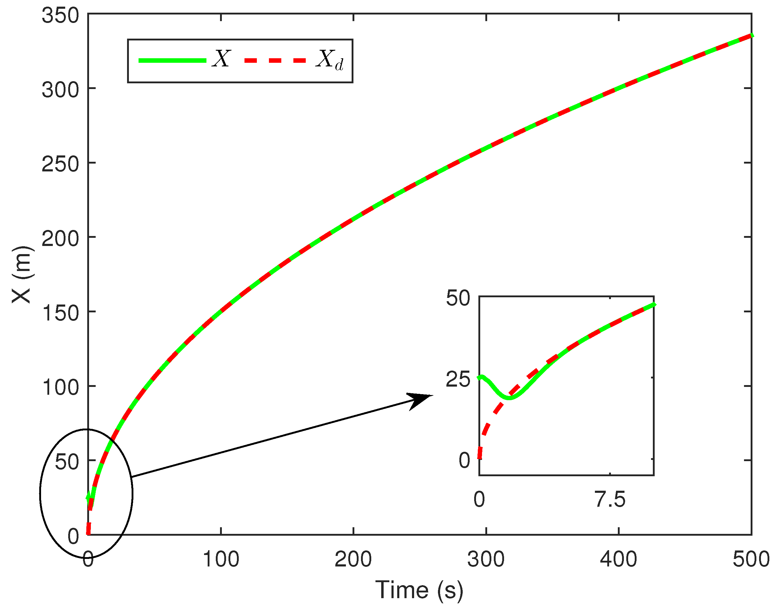
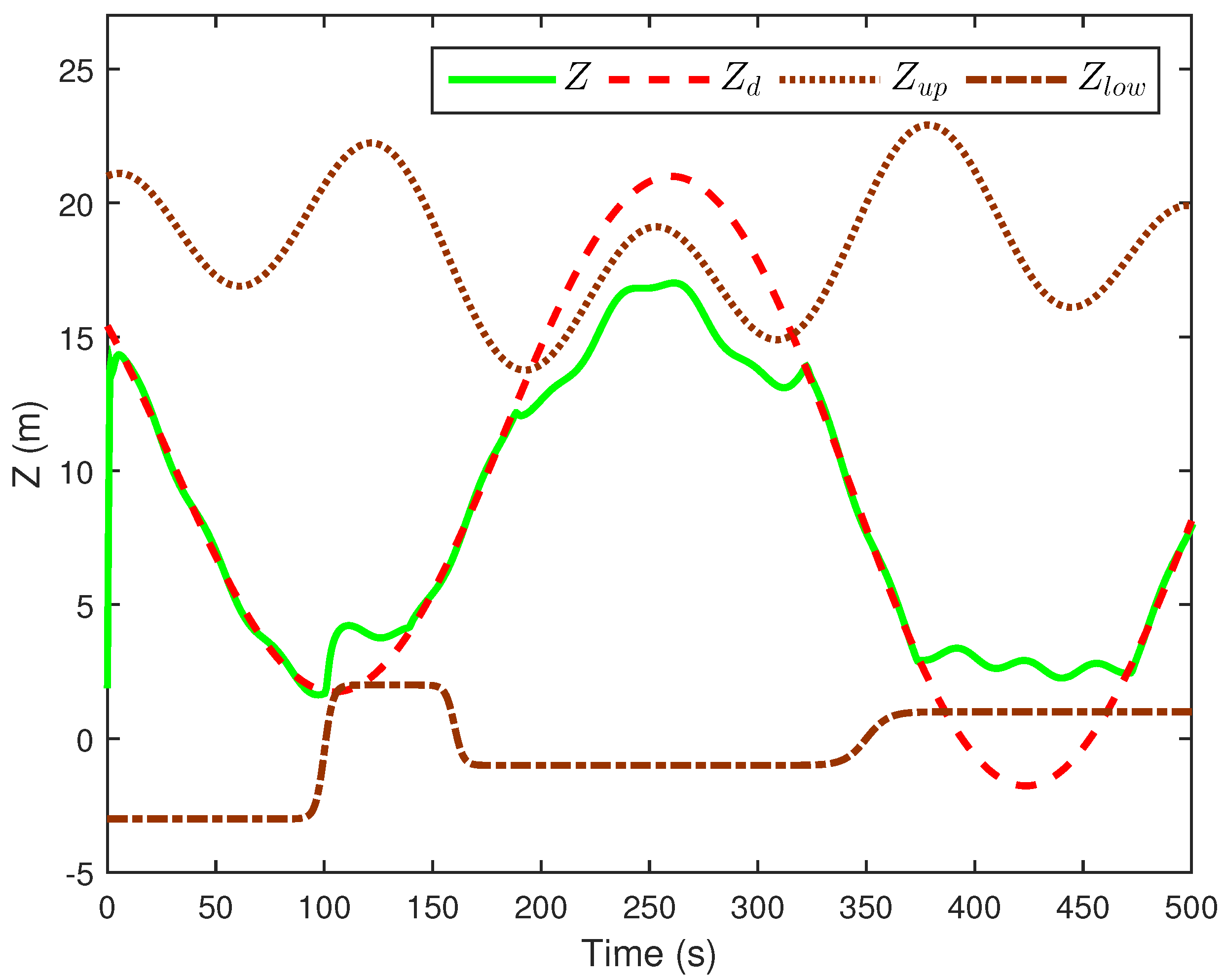
Figure 6, Figure 7 and Figure 8 express that P is able to track $P_d$ on the basis of satisfying the time-varying position boundaries. If the position boundaries conflict with $P_d$, the safety of the system has been considered first.

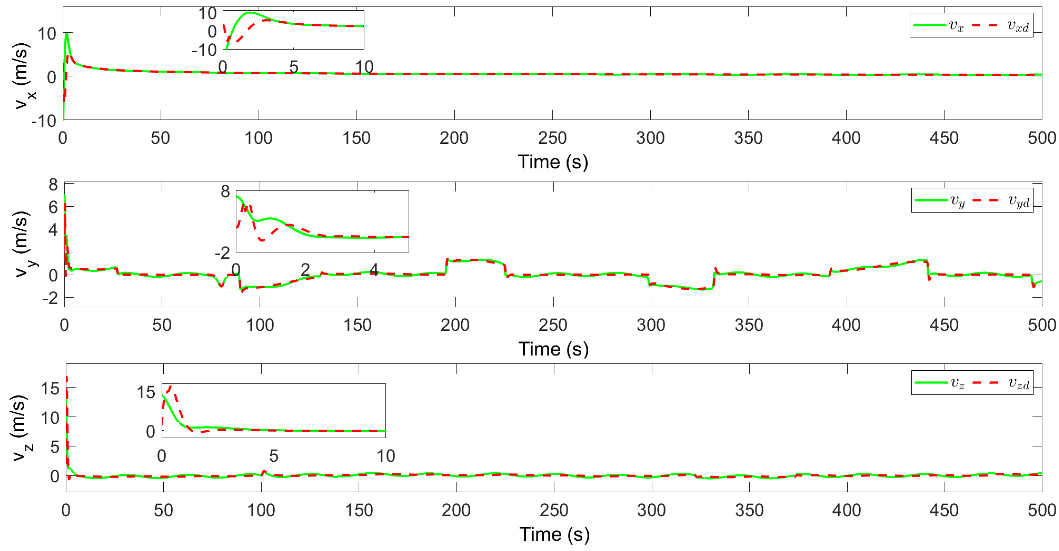
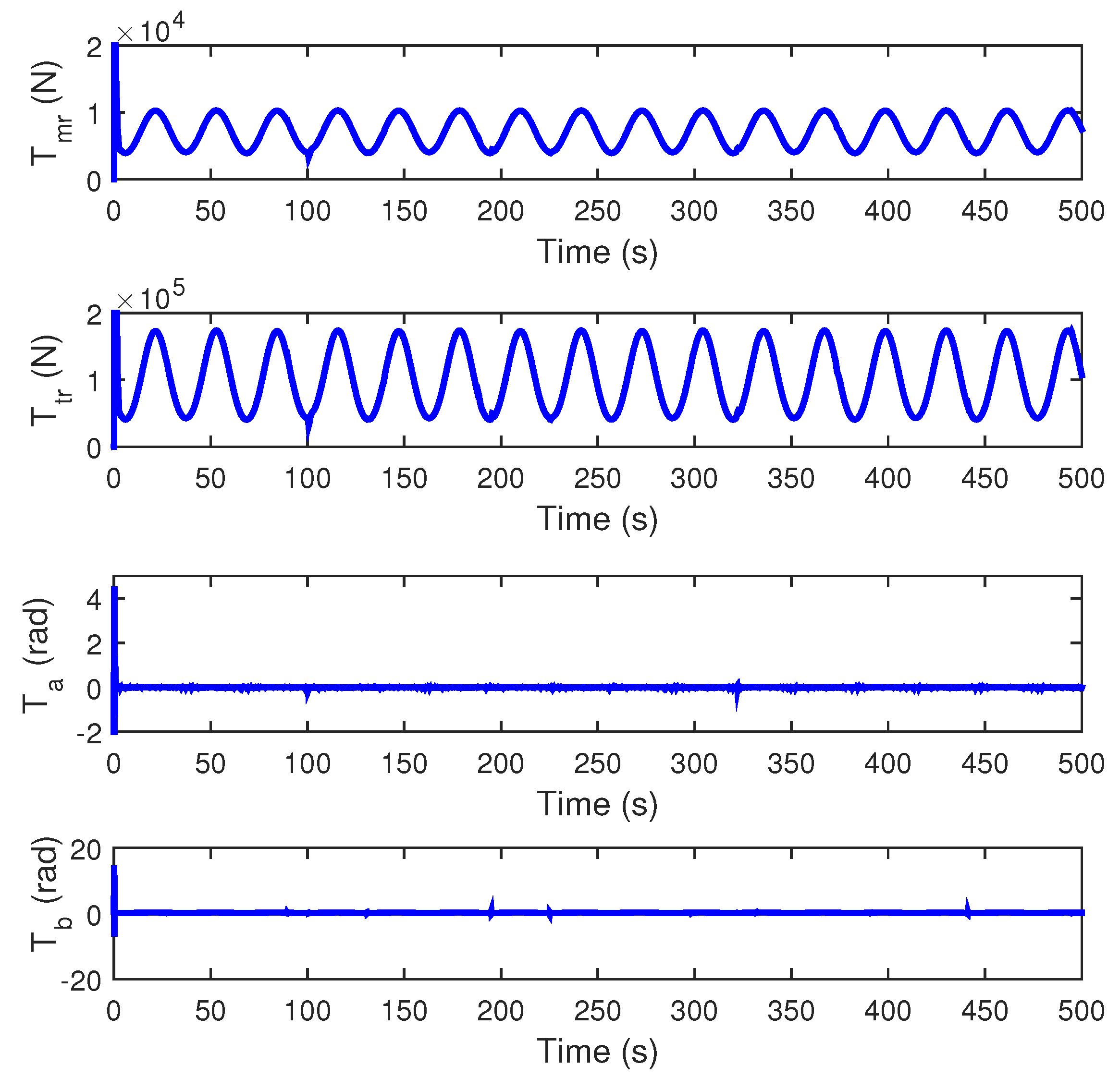
Figure 9, Figure 10, Figure 11 and Figure 12 show the tracking responses of v, $\mathrm{\Omega },\omega$, and $\chi$ and $v_d$, ${\mathrm{\Omega }}_d,{\omega }_d$, ${\chi }_d$. Figure 13 gives the response of the control inputs. As shown in Figure 9, Figure 10, Figure 11, Figure 12 and Figure 13, the proposed control scheme is able to guarantee the tracking performance of the UAH system. In addition, it can be observed that even though $T_{mr}$ and $T_{tr}$ oscillate a lot at the initial, they can quickly reach stability and meet the actual system requirements.

Figure 14 indicates a satisfying effect of the ESOs in (36), (50) and (60). To analyze the availability of the proposed control scheme, Figure 15 takes the position state in the Z-axis of the UAH as an example, which shows four different control schemes under the same condition and parameters. It can be seen that the proposed control scheme satisfies the control objectives as expected in green, while the control scheme without SPA in purple can not satisfy the time-varying path constraints $Z_{up}$, $Z_{low}$. Moreover, the control schemes without ESO in cyan can not track $Z_s$ accurately owing to the effect of disturbances. Simultaneously, the control scheme in [35] in yellow can constrain the desired signal within the safe range, and the time–time oscillation is too large, which cannot meet the needs of steady-state accuracy when the UAH is working.

It can be concluded that the simulation results above have classified that the proposed control scheme is available and effective for the UAH under time-varying path constraints and disturbances.

5. Conclusions

This paper purposes an ESO-based command-filtered safe flight control scheme for a 14-state unmanned helicopter system under time-varying path constraints and disturbances. A predictive mechanism has been added to the SPA to generate a new safe trajectory within the real-time path constraints. A command-filtered backstepping method is used to handle the piecewise differentiability. An ESO method is adopted to compensate unknown disturbances. The boundedness and safety of the closed-loop UAH system can be proved by a command-filtered backstepping technique and Lyapunov stability analysis. In addition, the performance of the proposed scheme is proved by numerical simulations.