Modal Analysis, Metrology, and Error Budgeting of a Precision Motion Stage


Department of Mechanical and Mechatronics Engineering, University of Waterloo, 200 University Avenue West, Waterloo, ON N2L3G1, Canada
*
Author to whom correspondence should be addressed.
J. Manuf. Mater. Process. 2018, 2(1), 8; https://doi.org/10.3390/jmmp2010008
Submission received: 18 December 2017
/
Revised: 12 January 2018
/
Accepted: 15 January 2018
/
Published: 24 January 2018
(This article belongs to the Special Issue Precision Manufacturing)
Abstract
:In this study, a precision motion stage, whose design utilizes a single shaft supported from the bottom by an air bearing and voice coil actuators in complementary double configuration, is evaluated for its dynamic properties, motion accuracy, and potential machining force response, through modal testing, laser interferometric metrology, and spectral analysis, respectively. Modal testing is carried out using two independent methods, which are both based on impact hammer testing. Results are compared with each other and with the predicted natural frequencies based on design calculations. Laser interferometry has been used with varying optics to measure the geometric errors of motion. Laser interferometry results are merged with measured servo errors, estimated thermal errors, and the predicted dynamic response to machining forces, to compile the error budget. Overall accuracy of the stage is calculated as peak-to-valley 5.7 μm with a 2.3 μm non-repeatable part. The accuracy measured is in line with design calculations which incorporated the accuracy grade of the encoder scale and the dimensional tolerances of structural components. The source of the non-repeatable errors remains mostly equivocal, as they fall in the range of random errors of measurement in laser interferometry like alterations of the laser wavelength due to air turbulence.
1. Introduction
Precision motion stages find extensive application in various industries for carrying out tasks related to manufacturing and inspection, as well as inside commercial products such as optical disk drives [1]. In this study, details of modal testing, laser interferometric metrology, and dynamic response to cutting forces, with subsequent error budgeting for a long-stroke linear nano-positioner is presented. A CAD drawing and photograph of the stage are presented in Figure 1. Some important features of design can be summarized as follows [2]:
- The nano-positioner utilizes a single shaft engaged to air bushings, instead of the more commonly used double shaft arrangement. The roll resistance is provided by the air bearing at the bottom. This way, the self-aligning property of the air bushings, which are held in the housings using O-rings, is exploited to the greatest extent, making the manufacturing and assembly of the stage easy and low-cost.
- Actuation is provided by two voice coil actuators (VCA) operating in moving magnet mode in complementary double configuration.
This paper performs a verification study of the nano-positioner, with emphasis on following a systematic approach. The methods can be applied in the metrology and dynamic analysis of similar precision motion systems that are used in precision and ultra-precision manufacturing.
The novel aspects of this work are summarized as follows:
- A modified ‘peak-picking’ approach has been developed which directly utilizes the accelerance measurement, through its modified formulations for the estimation of modal parameters. This way, the bias at low frequency, observed in the receptance plots obtained from accelerance via double integration, is avoided. Searching the modal analysis literature [3,4,5], the authors were not able to find a peak picking method which directly works with accelerance. With this study, we hope to fill in this gap.
- Modal testing, laser interferometric metrology, and error budgeting, although being established methods, have been applied to a novel precision motion stage design [2] for the first time. Outcome from these tests has allowed an in-depth evaluation of several design features regarding the overall accuracy and applicability of the motion stage in the micro-machining framework.
- A hybrid error budget has been compiled which combines the commonly considered quasi-static geometric, thermal, and steady-state servo errors with the dynamic component due to cutting forces. The 3-axis harmonic deflections due to machining forces, at the workpiece level of the stage, could only be predicted using the spatial modal testing results.
In the literature, several works can be found involving the identification of vibratory dynamics of high precision motion stages using finite element analysis (FEA) [6,7,8,9,10,11]. While in [6,7,8,10,11] a precision positioning stage or some of its components were analyzed, in [9] different design alternatives for an ultraprecision micro-milling machine are evaluated. In this paper, instead of FEA, modal analysis is carried out by direct experimentation using impact testing with a hammer and two different accelerometers. Two independent methods for conducting and evaluating the tests are employed, and their results are compared. The main purpose of modal testing has been to verify the dynamic properties of the stage and also facilitate response prediction to multi-axis dynamic disturbances, such as cutting forces, which cannot be directly predicted with model identification that is based only on control system input/output data.
A number of works on the measurement of error motions of precision motion stages have also been published [12,13,14,15,16]. A specially designed laser interferometer for measurement in all six motion axes was employed in [12]. In [13], error motions of a linear stage were measured by comparing results from a laser interferometer, an autocollimator, and capacitance probes. In [14], a two-degree-of-freedom linear encoder capable of simultaneously measuring linear positioning and horizontal straightness errors was used. In [15], out-of-straightness and axis misalignment errors of the carriage slide of a drum roll lathe are measured using two capacitance probes. Reflective-type optical sensors for on-line real-time measurements were proposed in [16]. In this study, error motions of a long-stroke linear nano-positioner are measured using a laser interferometer. Geometric errors obtained this way are combined with servo errors, estimated thermal errors, and the predicted dynamic response due to machining forces to compile the error budget.
The paper is organized as follows. In Section 2 predicted vibratory dynamics, the experimental modal testing and analysis methodology, as well as comparative results from the two independent methods are shown. In Section 3, the laser interferometric measurement procedure is described and the observed error motions are presented. In Section 4, the predicted error budget using the data available at the design phase is shown. Then, the actual error budget is established using the errors due to servo, geometric, thermal, and machining force factors. In Section 5, conclusions are presented.
2. Vibratory Dynamics
In this section, first, the predicted vibratory modes using information available at the design phase are presented. Then, experimental modal testing results are shown.
2.1. Predicted Vibration Modes
A schematic diagram of the motion stage is presented in Figure 2. Catalogue values of stiffness for the air-bushings/bearings [17] and certain dimensions are presented in Table 1. Inertia values of the moving body are calculated using CAD program and presented in Table 2. Flat air bearings are usually not rated for their rotational stiffness. At the time of conducting the design, due to the lack of rotational stiffness data or models concerning flat air bearings, a simple model as shown in Figure 3 was assumed, for estimating the air bearing reaction moment due to the rotational motion. When the stage body is in its rotationally neutral position, the assumed distributed stiffness elements () are preloaded.
The moment generated due to rotation can be expressed as:
where is the axial stiffness, and is the estimated rotational stiffness. The air bearing length () is different along the X and Z axes (, ), which results in different estimations for roll and pitch stiffness. It was observed later in the modal testing results presented in Section 2.6 that this approximation was not very accurate.
The natural frequency predictions for each significant vibration mode are presented in Table 3. For each motion axis, the natural frequency is found using the effective stiffness in that direction due to the bearings and the relevant mass or moment of inertia, using the analogy with a single-degree-of-freedom (SDOF) vibratory system [5]. The lowest predicted natural frequency is associated with the role mode at 538 Hz.
2.2. Summary of Modal Testing Methods
Modal testing of the linear nano-positioner is carried out using two independent methods as summarized in Table 4. The modified peak-picking approach which constitutes Method 1, has been developed as an alternative to the traditional peak-picking approach, with the primary difference being the usage of accelerance FRF directly, rather than converting to receptance first, which can introduce errors due to the measurement noise at low frequency. Details of how each method is employed are discussed in Section 2.3 and Section 2.4, for methods 1 and 2, respectively. Results are compared in Section 2.6.
2.3. Modal Analysis Method 1 (Modified Peak-Picking Approach)
2.3.1. Impact and Measurement Points
For method 1 (modified peak-picking), FRF measurements are taken in 3 different planes: XY, YZ, and XZ (Figure 4). For each measurement plane, accelerometer location and positive direction of acceleration measurement are indicated by , , and, . In each measurement plane, impact locations and directions are indicated by to for , to for , and to for .
2.3.2. Method of Analysis
In the first method, modal parameters, natural frequency () and damping ratio (), are identified using the developed ‘modified peak picking’ approach. ‘Peak-picking’, in the general sense, refers to the usage of graphical features of the real and imaginary parts of the FRF near the natural frequencies to estimate modal parameters [3,4,5]. Different resources may refer to slightly varying formulations of the ‘peak-picking’ method, although they share a similar basic idea. In this paper, a modified approach from traditional ‘peak-picking’ is taken in which the accelerance FRF is employed directly. The derivations of the formulas for this case are presented in the proceeding section side-by-side with formulas that have traditionally been used for receptance. Hence, by avoiding the numerical conversion from accelerance to receptance, the problem of double-integrating the low frequency noise can be largely circumvented through the use of the proceeding modified formulas.
Accelerance FRF between two coordinates (i and k) of a proportionally damped multi-degree of freedom (MDOF) system can be presented as a combination of vibratory modes as [3],
where, is the number of modes, and are the i-th and k-th elements of the r-th mode shape vector, is the natural frequency, is the damping ratio, and is the modal stiffness. In the case of a point FRF (), can be set without loss of generality, which makes equivalent to the static compliance contribution of each mode. The receptance for the same FRF () can be obtained from the accelerance as,
Equation (2) can be separated into real and imaginary parts as,
where represents the normalized frequency. If the modes are assumed to be separated from each other (i.e., having sufficiently distant natural frequencies), the real and imaginary plots of the FRF near each eigenfrequency () would resemble the characteristics of a single-degree-of-freedom (SDOF) system as shown in Figure 5 for both accelerance and receptance. Note that the extrema of the real and imaginary parts of the accelerance (, , ) around the natural frequency () attain close but different values than those for receptance (, , ), with the difference depending on the damping ratio (). However, the real part crossing of the abscissa is the same at for both cases.
Important characteristics of the real and imaginary plots of the FRF, and how they can be used to extract modal parameters (i.e., damping ratio, natural frequency, and modal participation factor) are summarized in the following, including the new steps proposed in our modified peak picking method:
- Setting yields two positive roots as, and . Hence, in our approach, the frequency values coinciding with the minimum and maximum real components of accelerance around the natural frequency () are used to determine the damping ratio as,
In traditional peak picking, extrema of the real component of receptance are considered, which occur at the following frequencies, leading to the corresponding damping ratio expression,
Figure 6a presents a comparison between the damping ratio values estimated from the real component of accelerance. When the proposed formulation in Equation (5) is used, the damping ratio is estimated correctly. However, if the traditional receptance formulation in Equation (6) is applied together with the approximation that and , then the damping ratio can only be estimated reasonably well if its actual value is 0.05–0.07 or less. In the case of the actual damping being higher, the use of Equation (6) yields a significant error when peak frequencies of real accelerance are substituted in place of their receptance counterparts. In the comparative modal testing results presented in Section 2.6, damping ratios as high as = 0.24 were encountered, with the vibration modes originating mainly from air bearing/bushing stiffness and damping properties. The receptance formulation in this case would have given incorrect estimates. Hence, the development of separate formulations for accelerance-based peak-picking was an obvious necessity in this study, and can be applied in other systems as well.
- ii.
- Setting yields only as the positive root. For , can be assumed. Hence, the imaginary peak/dip location is used to identify the natural frequency (). For receptance, the imaginary peak location is obtained as,
In Figure 6b, estimation of the natural frequency using accelerance versus receptance peak values is shown. It is observed that using the imaginary peak yields similar accuracy in both cases. Also, while the accelerance case overestimates, and deteriorates slightly faster for high values of , the receptance method underestimates the true . Overall, both methods are suitable for peak picking to a certain extent for their type of measurement.
- iii.
- Limit yields and 0. Hence, real part of accelerance has residues from the lower frequency modes, and using the horizontal axis crossing of for natural frequency estimation would be inaccurate.
- iv.
- Limit 0 yields 0 and 0. Hence, in accelerance, higher frequency modes typically do not have an influence on their lower frequency counterparts. In the case of receptance, the situation is reversed in which the higher frequency modes affect the real part only, and lower frequency modes exert very little influence.
For mode shapes to be identified, either the accelerometer location can be fixed and force impacts at different locations can be applied (roving hammer), or the impact location can be fixed while the accelerometer is placed at different points for each measurement (roving accelerometer). Due to the reciprocity rule (), results from the two cases should be equivalent in a linear system. Roving hammer measurements (for the same number of measurement points) can be carried out more quickly, as impacting at a point does not require any significant preparation. On the other hand, in the roving accelerometer case, more time is needed to properly mount the accelerometer at each measurement point, generally using wax. If one wants to determine mode shapes in three dimensions, which allows for a full three dimensional display of the vibratory motions, the response at every measurement point has to be measured in all three orthogonal axes. For the roving hammer case, this requires impacts in three orthogonal directions to be applied at each measurement point. This is very cumbersome; first, due to the difficulty of adjusting the orthogonal impact directions, second, due to the likelihood of some points being impossible to reach from all three directions. In such cases, it is much more advantageous to use a tri-axial accelerometer, which can output accelerations in all three axes at the same time, in roving accelerometer configuration. This way, both the problem of orienting measurement axes is solved, and the possibility of being obstructed by the measured structure is minimized, as the accelerometer is both smaller, and stays in place during measurement. In this paper, as the mode shapes are manually sketched in method 1, roving hammer configuration is used to obtain two dimensional mode shapes using hammer impacts from a single direction for each measurement point. On the other hand, taking advantage of the availability of three dimensional automated calculation and animation of mode shapes, in method 2, roving accelerometer configuration is used with a tri-axial accelerometer.
Denoting the accelerometer location as ‘o’, the accelerance FRF is given by . As the imaginary peak/dip approximately occurs at , the value of the peak/dip () can be expressed as:
Value of the imaginary peak/dip measured for a number of impact points, , can be related to the mode shape () as,
As the mode shapes, which are essentially eigenvectors of the system dynamics, can be scaled by any constant factor, the imaginary peak/dip values can be directly used for visualizing the elements of the mode shape vector. An example case of how the modes are sketched is illustrated in Figure 7, for the YZ measurement plane. The values of can be carried on the undeformed sketch of the structure using a graphical scaling factor. The deformed body is sketched using the displaced points, matching the displacements in their respective axes. For the actual analysis, additional points such as to are also considered.
2.4. Modal Analysis Method 2 (Software Package)
2.4.1. Impact and Measurement Points
The experimental setup for method 2 (software package) is presented in Figure 8a. In this method, the stage is impacted at the locations F1 and F2, as shown in Figure 8b. FRF’s are measured from the 3-axis accelerometer roved through –, which totals to 24 FRF’s for each impact point. A related module of Test.Lab® was used to acquire and view the FRF’s.
2.4.2. Method of Analysis
In method 2, modal identification has been carried out using automated and typically complex algorithms that have been documented in the literature, and implemented inside the commercially available vibration analysis software package. Natural frequencies and damping ratios were identified using the ‘PolyMAX’ module within LMS Test.Lab®. The proprietary ‘PolyMAX’ algorithm carries out a similar operation to the commonly used least-squares time domain complex exponential method, in the frequency domain [18]. The resulting stabilization diagram is interpreted for natural frequencies and damping ratios. For constructing the mode shapes, these identified parameters are used in the least-squares frequency domain (LSFD) algorithm [19], which finds the best fit to the modal displacement vector based on the agreement between the measured and fitted FRF’s. The software package allows either complex or real mode shapes to be fit. In this paper, complex mode shapes are enabled to test the proportional damping assumption. Complexity of mode shapes is rated using ‘modal phase collinearity ()’ and ‘mean phase deviation ()’ [19]. and rate the complexity of the mode on a scale 0 to 100%, and 0°–90°, respectively. Having obtained a minimum of 96.5%, and a maximum of 12° in the set of identified mode shape vectors, the proportional damping assumption used in method 1 (Section 2.3) is observed to be justifiable. Identified mode shapes can be animated as a 3D video, and screenshots of the animated mode shapes are presented in Section 2.6.
2.5. Measurements from the Encoder
For the identification of axial modes in the X-direction or modes which have significant displacement components along the stage’s direction of sensitivity, measurements that are parallel to the encoder axis are needed. Such modes are critical for the positioning control stability, as they directly enter the control loop through the encoder measurement. In this regard, position readings from the encoder scale, evaluated by the DSpace® DS3002 encoder interface board, were fed to CutPRO®’s MalTF interface, as a position measurement, using the DS2102 digital to analog converter. The boards (DS3002, DS2102) ran at sampling frequency of 20 kHz. The same impact points in three planes mentioned for method 1 (Figure 4) were used, with the accelerometer replaced by the encoder. Receptances acquired this way did not yield any vibratory modes in the 0–2000 Hz range. Eventually, position control bandwidth in the X-axis could be increased up to 650 Hz without experiencing any interactions with vibratory modes, affirming these results. The bandwidth was mainly limited by the phase advance that can be contributed by the control scheme at the desired cross-over frequency, while ensuring that amplification of measurement noise through feedback did not display a significantly deteriorating effect.
2.6. Comparative Results and Discussion
Comparative modal testing results from method 1 (modified peak-picking) and method 2 (LMS Test.Lab®) are presented in Figure 9, along with natural frequency predictions made at the design phase (Section 2.1). It is observed that the identified natural frequencies for methods 1 and 2 are rather close, except for a slightly larger deviation for the first mode. Damping ratios are also observed to be close. On the other hand, large discrepancies between the experimentally identified and predicted natural frequencies can be noticed. This discrepancy is especially critical in the case of the first mode (roll). While methods 1 and 2 have measured 65 Hz and 79 Hz, respectively, the initial theoretical prediction was 538 Hz. The roll motion is only constrained by the flat air bearing at the bottom, and such bearings are usually not rated for rotational stiffness.
For the theoretical calculations, a simple model assuming distributed stiffness was used. Apparently, the actual rotational stiffness of the air bearing is much lower than approximated, which can be attributed to the distortion of the air cushion at the bearing interface and changing air flow conditions dependent on fly height and orientation. In order to make more accurate predictions, more detailed analyses and data on the rotational stiffness of the air bearing is necessary.
Identified modes 2 (horizontal) and 3 (vertical) also imply deviation of the actual vibratory dynamics from the predicted ones. The fact that natural frequencies measured for these two modes are close suggests symmetry in the actual system in the horizontal and vertical directions. On the other hand, such symmetry was not predicted due to the assumed contribution of the flat air bearing stiffness in the vertical direction. The effective normal stiffness of the air bearing appears to be lower than the catalogue value, which may be due to a higher gap in the final assembly. The air bearing still provides some stiffness, as evident from the slightly higher natural frequency identified for the vertical mode (mode 3). The reason for both modes 2 and 3 having lower natural frequency than expected can be due to a lower effective stiffness of the air bushings, likely due to the shaft being manufactured closer to the minimum diameter within the tolerance range.
Contrary to the other modes, the natural frequency identified for mode 4 (pitch) is higher than the theoretical prediction. When the main compliances causing a vibratory mode shape are due to the bearings, mode shapes assume rigid-body motion-like patterns, as assumed for the theoretical predictions. However, motions in each degree of freedom (linear and rotational axes) are not totally decoupled as it was assumed. This can be observed in modes 3 and 4, which have motions in both vertical and pitch directions. This can be the reason mode 4 attained a higher natural frequency than expected. Also, elastic deformations of the structural components couple with bearing compliances to alter vibratory dynamics. Mainly elastic modes were not identified in the 0–2000 Hz range, but a dominantly axial elastic mode was identified at 2765 Hz using method 1.
Overall, these modal measurements help assess the validity of many of the assumptions made during the design phase, and also highlight what additional knowledge is needed for making more realistic predictions. They also allow the response to a complex disturbance input to be evaluated in a fairly detailed manner, as performed in Section 4.2.3.
The procedure outlined in this section can be applied to other similar motion systems as follows:
- For a quick and straightforward assessment of the most prominent vibration modes (starting from the first mode) the ‘peak-picking’ procedure can be applied, as it is shown to yield sufficient accuracy. This information can be incorporated in the determination of the control bandwidth.
- For further investigation of the vibratory dynamics, typically with >5 modes, as well as for the representation of mode shapes in three dimensions, a software package similar to the one utilized in this paper can be used.
- Results from the two methods can be combined in the assessment of design features, like the magnitude and geometry of the compliances of the stage and bearings, as exemplified in this study by the less than ideal roll resistance observed through modal testing.
3. Laser Interferometric Metrology
Laser interferometric metrology has been used to measure the geometric errors along the linear path of the motion stage using varying combinations of the laser source and the measurement optics (retroreflector, Wollaston prism, straightness retroreflector, angular retroreflector). The results from this section are used in compiling the error budget in Section 4.
3.1. Methodology of Measurements
Definitions for the machine tool coordinate system and the error motions are presented in Figure 10 [20]. Measurement target positions are chosen with some randomness in the spacing between each other as recommended in the standard [21], and are presented in Table 5. The stage dwells for 2 s at each position, and the average of measurement between 1.0–1.8 s is used. Each point is crossed 5 times in backward and forward directions.
During the tests, ambient pressure, temperature, and relative humidity were monitored. These values were later used in the Edlen equation [22] to obtain the laser wavelength. The locations of the measurement optics with respect to the center of gravity of the stage are presented in Figure 11. Abbe compensation is applied to the linear measurements using the angular measurements and the moment arms to bring them to the common point at the center of gravity. Linear errors in each axis can be expressed in terms of angular deviations and the 3D rotation matrix simplified for small angular deviations [23] as,
where are the linear errors, are the angular deviations in each rotation axis, and are the moment arms.
3.2. Evaluation of the Results
The deviation at each point is given by where i = 1, …, 18 is the index of measurement position and j = 1, …, 5 is the index of pass. Forward (), backward (), and unidirectional () mean positional deviations are expressed as:
The estimator of standard uncertainty is found as,
where the backward direction () version is found by replacing () with (). For each error measurement, a standard final plot with deviations at each point at each pass (), mean deviations (, , ), and mean deviations with uncertainty range (, ) are produced. The rest of the parameters related to accuracy and their definitions are presented in Table 6 [21].
3.3. Measurement Results
Linear and angular accuracies are presented in Table 7 and Table 8, respectively, as PV magnitudes. Detailed discussion of each error component is presented in the subsequent sections.
3.3.1. Linear Positioning Error (EXX)
Measurement results for EXX are presented in Figure 12. Abbe compensation is applied by adding the multiplication of the pitch error (ECX) by the 18.5 mm moment arm shown in Figure 11a, to the raw measurement result. The moment arm is measured from the encoder position, as the positioning error of the encoder scale w.r.t. the center of gravity is taken care of by the servo. The uncertainty of measurement due to the misalignment of the laser beam is given in the standard [21] as:
where is the uncertainty in (μm), is the misalignment in (mm), and is the measurement length in (m). As the laser encoder system used [24] provides an LED lamp for the indication of the level of alignment, < 1 mm can be assumed [21]. On the other hand, this still implies up to 15 μm possible error. Hence, the approximately 2 μm total slope removed from the Abbe compensated EXX (Figure 12b) can easily be the cosine error due to misalignment, justifying its removal. Alternatively, it can be due to the encoder scale not being mounted at an absolute right angle to the motion stage axis. In the latter case, it is an actual error rather than a measurement error and it should not be removed. However, it would still be a repeatable error that can be compensated by shifting the position reference.
After the removal of the slope, the bidirectional systematic error is given by = 1.2 μm (Table 7). It is compatible with the expectations as the Heidenhain® LIP501 R encoder scale is graded for ±1 μm accuracy [25], which corresponds to PV 2 μm possible error. The repeatability is evaluated as = 0.7 μm, which is poorer than expected for the typical optical encoder. Considering the approximately 300 mm dead path, the repeatability corresponds to about ±1 ppm deviation, which can be attributed to environmental disturbances on the laser measurement, such as the turbulence of the ambient air. Altogether, the accuracy is evaluated as = 1.8 μm.
3.3.2. Straightness Error in Y (EYX)
Measurement results for EYX are presented in Figure 13. Abbe compensation has been applied to the raw results by subtracting the multiplication of the pitch error (ECX) by the 45.5 mm moment arm. As straightness measurements are prone to large errors due to the misalignment of the straightness retroreflector, the constant slope portion has been removed after Abbe compensation (Figure 13c). EYX results indicate a possible curvature on the main shaft, which might have been introduced during the machining of the flat surfaces, used for mounting the top and bottom plates. A least-squares best fit line has been used to shift the zero of the deviations axis. The repeatability of = 0.5 μm is more likely due to laser measurement errors as in EXX. An overall accuracy of = 2.5 μm has been measured.
3.3.3. Straightness error in Z (EZX)
Measurement results for EZX are presented in Figure 14. Abbe compensation has been applied by adding the multiplication of the yaw error (EBX) by the 45.5 mm moment arm to the raw result. As in EYX, the slope due to the misalignment of the optics is removed and the reference is shifted to the least-squares best fit line. A repeatability of = 0.9 μm and overall accuracy of = 1.6 μm are observed.
3.3.4. Yaw Error (EBX)
Measurement results for EBX are presented in Figure 15. A repeatability of = 3.4 μm/m and an accuracy of = 7.2 μm/m have been obtained. As the angular measurements are immune to misalignment errors, no corrections of the raw results have been made.
3.3.5. Pitch Error (ECX)
4. Error Budget
The error budget is made up of components related to geometric, thermal, and servo errors, as well as the dynamic response due to machining forces. In this section, first, a predicted error budget is presented which uses nominal properties of the components. Then, measured/estimated actual errors are used for the actual error budget. Results from the two cases are compared.
4.1. Predicted Error Budget
In the predicted error budget, peak-to-valley (PV) error magnitudes are used likewise the actual one. The items included can be summarized as follows:
- The PV error due to position sensor resolution is given by = 0.97 nm, derived from the 4096 times arctangent interpolation of the 4 μm measurement signal period.
- The linear encoder scale is rated for ±1 μm grating error [25], hence the PV error due to encoder grating defects is given by = 2000 nm.
- The main shaft of the motion stage acts as the guideway for the air bushings. It is manufactured to a cylindricity tolerance of 5 μm as shown in Figure 17. Assuming that roughly half of the possible errors due to the errors in the shaft dimension are cancelled by its realignment in the air gap, PV errors in Y and Z directions can be assumed to be = 2.5 μm, and = 2.5 μm, respectively.
The predicted error budget is presented in Table 9. The PV predicted error is 4.1 μm. The rationale behind using the sum of root-mean-square (RMS) values and the final prediction being the mean of the arithmetic and RMS sums has been explained in Section 4.2.4.
4.2. Actual Error Budget
4.2.1. Geometric Component
Summary of geometric accuracies w.r.t. the center of gravity are presented in Table 10. When it is assumed that compensation of the systematic error in all 5 axes is possible, i.e., if the actuator is used as part of a multi-axis micro machine-tool, the geometric errors reduce to just the repeatability value. In the error budget, both cases are considered separately to demonstrate the extent to which the system can be corrected with compensation.
4.2.2. Thermal Component
Thermal Disturbance Sensitivities
The linear nano-positioner body is made up of aluminum, steel, permanent magnet material, and encoder glass. A diagram showing key variables relevant to thermal disturbance sensitivities is presented in Figure 18. The point of interest is defined at the center of the upper surface of the top plate as shown.
The point of interest is sensitive to the following thermal disturbances:
- In the case of thermal expansion along the X-axis, combined effect of the expansion of the encoder scale and the top plate needs to be considered. If the encoder scale is thought of as fixed at its center to the top plate, the deviation in X-positioning would be represented by,where is the coefficient of thermal expansion of the glass encoder scale specified by the manufacturer [25], and is the coefficient of thermal expansion of Aluminum 6061. On the other hand, the encoder scale is held by clamps which do not exert a significant pressure on the scale and the scale can be thought of as decoupled from the top plate. In that case, X-axis positioning error needs to be revised as,which corresponds to a worse scenario due to > .
- Along the Y-axis, thermal expansion of the stage would push the point of interest upwards bywhere is the thickness of the stage, and is the temperature variation. If the stage body was only constrained by the air bearing at the bottom, the thermal expansion would be . As the air bushings are expected to counteract this, is used to approximate the equilibrium position.
- Thermal expansion along the Z axis does not affect the point of interest.The thermal sensitivity in X and Y axes can be defined as,The total linear thermal sensitivity of positioning can be expressed as,
Values of the thermal sensitivities and parameters used in calculations are summarized in Table 11.
Thermal Disturbances and the Resulting Thermal Error
At the specified peak current, VCA’s dissipate 1.19 W each, which can result in considerable thermal disturbances in a micro/nano-precision setting. The thermal stability of the nano-positioner is tested using a jerk limited cubic acceleration profile trajectory with the maximum acceleration, A = 5000 mm/s2 (which is slightly short of the maximum achievable acceleration of 6480 mm/s2), and the resulting high feedrate, F = 200 mm/s, constrained by the stroke length limitation. With a 0.05 s dwell period prescribed at the far end of the stroke, the period of back and forth motions is determined as 0.35 s. Thermocouples were mounted at the adjustment ring near the VCA core and the top plate on the main shaft. The stage was run for 8 h, for which the collected temperature readings are presented in Figure 19.
From the plot, it can be inferred that after the initial warming-up phase, temperature keeps rising steadily at a rate of approximately 0.1 °C/h. As the adjustment ring is closer to the VCA’s, it heats up in advance. The ambient temperature could possibly be kept steadier with better air-conditioning and ventilation equipment, which would also contribute to the cooling of the stage. However, the proximity of equipment such as the amplifiers, voltage supply, controller, and the PC to the experimental setup makes it a challenge. It should also be noted that the compressed air supply at the air-bushing/shaft interface contributes to the cooling of the stage due to the high heat transfer coefficient associated with the forced convection in the resulting annular duct. However, this effect does not amount to an observable isolation of the top plate from the heat generated by the VCA’s, due to the low flow rate of the air bushings. Assuming that the micro-milling operation for which the nano-positioner is intended can involve a calibration cycle every 2 h., thermal variation of the stage can be budgeted using = 0.2 °C. Hence, the resulting dimensional error is given by = 92 nm.
4.2.3. Machining Force Component
Machining forces contribute to motion errors by causing dynamic deflections (i.e., vibrations). The directions of anticipated machining force components acting on the payload were presented in Figure 1. The machining force input in the X-direction enters the control system as shown in the block diagram of Figure 20 [2]. In the block diagram, (A/V) is the current control response, (N/V) is the actuator force factor, stands for the rigid body dynamics of the actuator body floating on the air bearings, and stands for the vibratory modes in the axial direction. The overall plant is given by,
which was measured using frequency response, for controller design purposes. The dynamic compliance in the axial direction is given by the control system’s disturbance rejection function () as,
where can be set in the 0–2000 Hz range, as the measurements of Section 2.5 revealed no vibration modes.
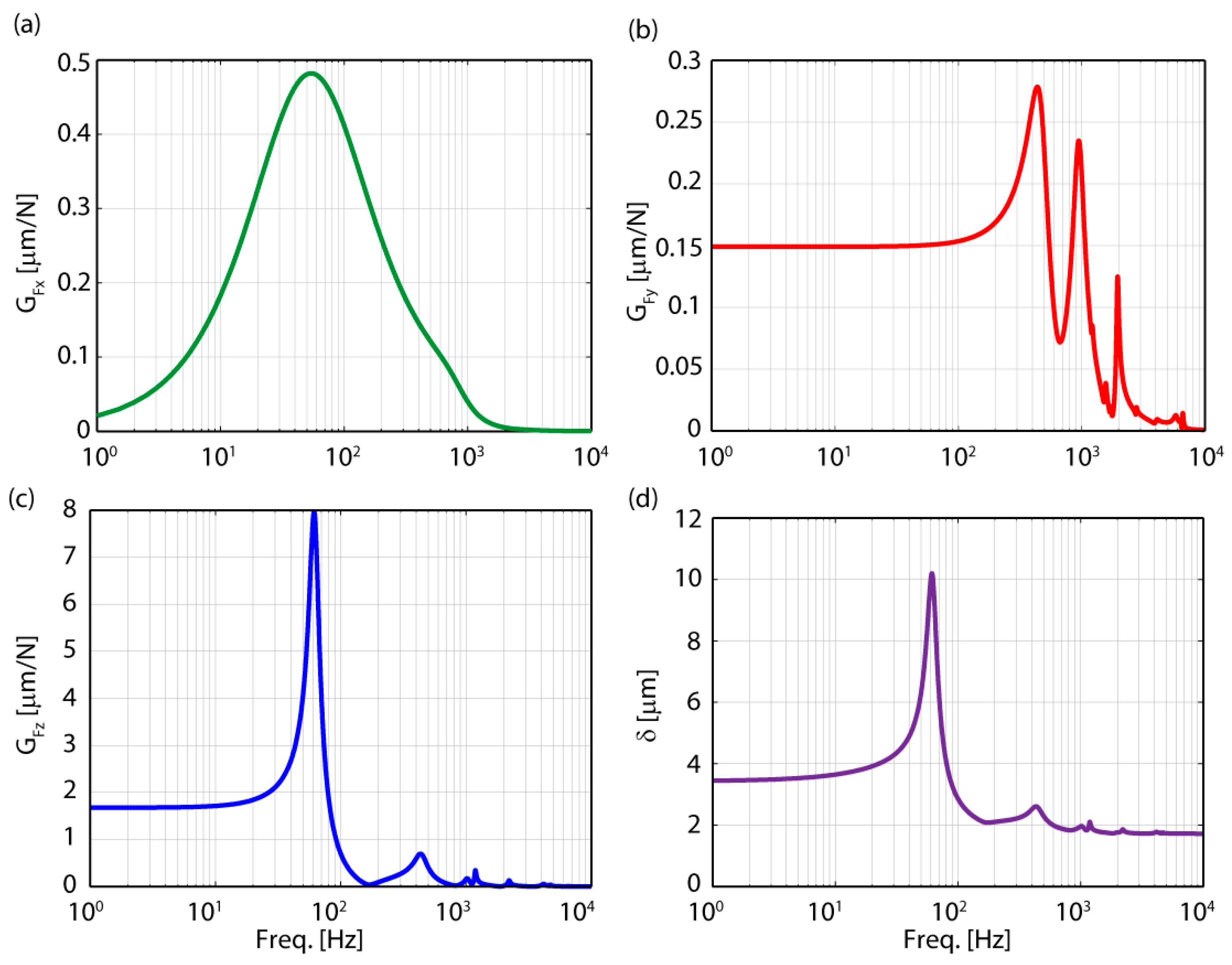
In the case of and , dynamic compliances are given by the deformability of the structure as a function of the excitation frequency, which was captured in the FRF measurements in Section 2. Referring to Figure 4, FRF measured between F”1-Axy can be used as , and the FRF measured between F1-Axz can be used as . As the FRF’s are measured in terms of accelerance, conversion to receptance needs to be carried out for the position response. Instead of directly dividing the accelerance magnitudes by the square of the frequency (as suggested by the mathematical definition), receptances are synthesized from modal parameters which were fitted using peak-picking, in order to prevent distortions in the low-frequency region. Resulting , , are presented in Figure 21a–c. The compliance in the Z-direction is about an order of magnitude higher than the others, due to the low effective roll resistance provided by the flat air bearing, as discussed in Section 2.6.
For the quantification of forces, a slotting case was considered with sinusoidal force components as follows:
The resulting deflections can be obtained from . Phase differences in the timing of the forces can be neglected for a worst-case scenario to obtain the total deflection as,
Depending on the nature of the cutting operation, the above force model may of course be replaced with a more suitable one as needed [26,27]. The resulting deflection () as a function of the excitation frequency is presented in Figure 21d. The reported values comprise both the static response to the constant part and the sinusoidal part which changes as a function of the spindle frequency. In micro-milling, due to the compliance of the tools used, the machining forces are limited to 1–2 N in order to obtain the desired tolerances in the finished part. This is achieved by limiting the chip load using high spindle speeds [28]. Assuming a 2 teeth cutter, and a spindle speed of 50,000 rpm, a tooth passing frequency of = 1667 Hz is obtained, for which the total deflection is given by = 1.748 μm.
4.2.4. Compilation of the Error Budget
The error budget is presented in Table 12. Original errors are presented at the left, and non-repeatable errors after the assumed ideal geometric compensation are presented at the right. Servo error is obtained from trajectory following tests conducted with the stage. Thermal errors and machining force deflections are considered as non-repeatable. The error budget is compiled for the point of interest at the center of the top plate, therefore EXX is modified from the values obtained for the center of gravity (Table 10) using the Abbe moment arm and ECX.
When combining errors, the arithmetic sum gives the worst case, while the RMS sum provides a more realistic figure, assuming that the different error sources are probabilistic and not correlated. In practice, average of the two is used as a suitable estimate [29]. For the RMS sum to be applicable, variance of the presented error components has to be found, instead of PV magnitude. Assuming a uniform probability distribution centered at zero, RMS sum of the errors can be expressed as [30]:
where are the individual PV errors.
The error budget indicates a PV 5.7 μm deviation with the repeatable errors conserved, and 2.3 μm when 5 DOF compensation is assumed to be available. With these results, the nano-positioner can be concluded to be marginally suitable for micro-milling applications. Comparing measured values to the estimations from Section 4.1, linear and straightness errors are observed to be of similar magnitude. The non-repeatable parts observed in measurement were not anticipated in predictions. The source of non-repeatable errors is mostly equivocal, as they fall in the range of random errors of measurement in the applied laser interferometric method, for example due to the turbulence of ambient air. The systematic part of the errors in Y and Z axes are smaller than predicted, as the predictions employed the whole tolerance range of the shaft. In reality, within the tolerance range, the shaft may be manufactured to a better uniformity. In EXX, the systematic error measured is larger than estimated error due to the observed curvature of the shaft mostly evident in the EYX and ECX measurements. This affects the point of interest through the moment arm. Servo and thermal errors are observed to contribute a relatively small portion of the overall error. Dynamic deflections due to machining forces are anticipated as a major component of the error, mostly due to the compliance in the roll direction.
The error budget represents data that goes into the core of the performance specifications for a precision motion stage, in terms of accuracy. As such stages also constitute motion axes of micro-/nano-machine tools, they directly affect the achievable manufacturing accuracy. In this study, modal testing has been incorporated in the error budget to determine the dynamic deflections due to machining forces, in this regard. The new procedures proposed in this paper (i.e., modified peak picking method and merging of dynamic response predictions into an error budget) are applicable to a wide set of precision motion stages and machine tools.
5. Conclusions
The long-stroke linear nano-positioner design has been verified through modal testing, and laser interferometric measurements with subsequent error budgeting. The lowest resonance is observed to be a roll mode at 65 Hz, which was predicted to occur at 538 Hz before the stage was built. It is inferred that the roll/pitch resistance of the flat air bearing is much lower than the prediction, which highlights the need for additional data and modeling tools to aid designers of precision equipment. Nevertheless, this roll mode did not have any negative influence on the servo performance of the stage, which could achieve 450–650 Hz crossover frequency [2].
The error budget concludes PV 5.7 μm accuracy, which has a non-repeatable part of PV 2.3 μm. Systematic part of the errors could be reasonably predicted at the design phase, and they came more or less from the manufacturing tolerance and the assembly process. The semi-circular trend in the motion most likely originates from a curvature on the main shaft. There has also been a degree of uncertainty regarding the origin of the non-repeatable geometric errors. In the future, investment into better environmental control in the laboratory may help obviate some of the random sources of laser interferometric measurement error.
Overall, the modal analyses, laser interferometry, spectral analysis, and error budgeting has enabled the validation of many of the assumptions and predictions made during the design of the precision stage. The measurements and analyses have also clearly indicated the limitations of, and possible improvements to, this type of linear motion stage, such as enhancing the stiffness in the roll direction. The results further demonstrate the need for additional modelling capability and data regarding the multi-directional stiffness behavior of porous flat air bearings.
Acknowledgments
The authors would like to thank B. Tryggvason for his inputs into the development of the precision stage, and also University of Waterloo technicians R. Wagner and N. Griffett for their meticulous assistance in building and instrumenting it. This work was supported by the Natural Sciences and Engineering Research Council of Canada (NSERC) through Discovery grant RGPIN-03879 and Engage grant EGP #436910-12.
Author Contributions
This research has been carried out by Ahmet Okyay, as part of his PhD studies under the supervision of Kaan Erkorkmaz and Mir Behrad Khamesee. The supervisory roles of Kaan Erkorkmaz and Mir Behrad Khamesee included, but were not limited to, the structuring of the research problem, determination of the methods, advice on the relevant literature, direct participation in certain experiments, and the evaluation of results. The bulk of the research results have been obtained, and the write-up of the paper has been carried out by Ahmet Okyay with substantial editorial suggestions from the other authors.
Conflicts of Interest
The authors declare no conflict of interest.
References
- Tan, K.K.; Lee, T.H.; Huang, S. Precision Motion Control: Design and Implementation, 2nd ed.; Springer: Berlin, Germany, 2008. [Google Scholar]
- Okyay, A. Mechatronic Design, Dynamics, Controls, and Metrology of a Long-Stroke Linear Nano-Positioner. Ph.D. Thesis, University of Waterloo, Waterloo, ON, Canada, 2016. [Google Scholar]
- Ewins, D.J. Modal Testing: Theory and Practice; RSP: Taunton, UK, 1986. [Google Scholar]
- Schmitz, T.L.; Smith, K.S. Machining Dynamics: Frequency Response to Improved Productivity; Springer: Berlin, Germany, 2009. [Google Scholar]
- De Silva, C.W. Vibration: Fundamentals and Practice; CRC Press: Boca Raton, FL, USA, 1999. [Google Scholar]
- Chang, S.H.; Tseng, C.K.; Chien, H.C. An ultra-precision XYθZ piezo-micropositioner, I. design and analysis. IEEE Trans. Ultrason. Ferroelectr. Freq. Control 1999, 46, 897–905. [Google Scholar] [CrossRef] [PubMed]
- Tenzer, P.E.; Mrad, R.B. A systematic procedure for the design of piezoelectric inchworm precision positioners. IEEE-ASME Trans. Mechatron. 2004, 9, 427–435. [Google Scholar] [CrossRef]
- Dong, W.; Tang, J.; ElDeeb, Y. Design of a linear-motion dual-stage actuation system for precision control. Smart Mater. Struct. 2009, 18, 095035. [Google Scholar] [CrossRef]
- Huo, D.; Cheng, K.; Wardle, F. A holistic integrated dynamic design and modelling approach applied to the development of ultraprecision micro-milling machines. Int. J. Mach. Tool Manuf. 2010, 50, 335–343. [Google Scholar] [CrossRef]
- Moon, J.H.; Pahk, H.J.; Lee, B.G. Design, modeling, and testing of a novel 6-dof micropositioning stage with low profile and low parasitic motion. Int. J. Adv. Manuf. Technol. 2011, 55, 163–176. [Google Scholar] [CrossRef]
- Li, Y.; Huang, J.; Tang, H. A compliant parallel xy micromotion stage with complete kinematic decoupling. IEEE Trans. Autom. Sci. Eng. 2012, 9, 538–553. [Google Scholar] [CrossRef]
- Liu, C.H.; Jywe, W.Y.; Hsu, C.C.; Hsu, T.H. Development of a laser-based high-precision six-degrees-of-freedom motion errors measuring system for linear stage. Rev. Sci. Instrum. 2005, 76, 055110. [Google Scholar] [CrossRef]
- Gao, W.; Arai, Y.; Shibuya, A.; Kiyono, S.; Park, C.H. Measurement of multi-degree-of-freedom error motions of a precision linear air-bearing stage. Precis. Eng. 2006, 30, 96–103. [Google Scholar] [CrossRef]
- Kimura, A.; Gao, W.; Lijiang, Z. Position and out-of-straightness measurement of a precision linear air-bearing stage by using a two-degree-of-freedom linear encoder. Meas. Sci. Technol. 2010, 21, 054005. [Google Scholar] [CrossRef]
- Lee, J.C.; Gao, W.; Shimizu, Y.; Hwang, J.; Oh, J.S.; Park, C.H. Precision measurement of carriage slide motion error of a drum roll lathe. Precis. Eng. 2012, 36, 244–251. [Google Scholar] [CrossRef]
- Lee, H.W.; Liu, C.H. High precision optical sensors for real-time on-line measurement of straightness and angular errors for smart manufacturing. Smart Sci. 2016, 4, 134–141. [Google Scholar] [CrossRef]
- New Way Air Bearings. Catalogue; New Way Air Bearings: Aston, PA, USA, 2017; Available online: http://www. newwayairbearings.com/catalog/components (accessed on 17 January 2018).
- Peeters, B.; Van der Auweraer, H.; Guillaume, P.; Leuridan, J. The polymax frequency-domain method: A new standard for modal parameter estimation? Shock Vib. 2004, 11, 395–409. [Google Scholar] [CrossRef]
- Heylen, W.; Lammens, S.; Sas, P. Modal Analysis Theory and Testing; Department of Mechanical Engineering, Katholieke Universiteit Leuven: Leuven, Belgium, 1995. [Google Scholar]
- International Organization for Standardization. ISO/DIS 230-1 Test Code for Machine Tools, Part 1: Geometric Accuracy of Machines Operating Under No-Load or Quasi-Static Conditions; ISO: Geneva, Switzerland, 2009. [Google Scholar]
- International Organization for Standardization. ISO 230-2 Test Code for Machine Tools, Part 2: Determination of Accuracy and Repeatability of Positioning Numerically Controlled Axes; ISO: Geneva, Switzerland, 2006. [Google Scholar]
- National Institute of Standards and Technology (NIST). Engineering Metrology Toolbox; NIST: Gaithersburg, MD, USA, 2017. Available online: http://emtoolbox.nist.gov/Wavelength/Edlen.asp (accessed on 17 January 2018).
- Kuipers, J.B. Quaternions and Rotation Sequences: A Primer with Applications to Orbits, Aerospace, and Virtual Reality; Princeton University Press: Princeton, NJ, USA, 1999. [Google Scholar]
- Renishaw. RLE Fiber Optic Laser Encoder; Renishaw: Hong Kong, China, 2015. [Google Scholar]
- Dr. Johannes Heidenhain GmbH. Exposed Linear Encoders; Dr. Johannes Heidenhain GmbH: Traunreut, Germany, 2000. [Google Scholar]
- Altintas, Y. Manufacturing Automation: Metal Cutting Mechanics, Machine Tool Vibrations, and CNC Design, 2nd ed.; Cambridge University Press: New York, NY, USA, 2012. [Google Scholar]
- Chae, J.; Park, S.S.; Freiheit, T. Investigation of micro-cutting operations. Int. J. Mach. Tool Manuf. 2006, 46, 313–332. [Google Scholar] [CrossRef]
- Cheng, K.; Huo, D. (Eds.) Micro-Cutting: Fundamentals and Application; John Wiley & Sons: Hoboken, NJ, USA, 2013. [Google Scholar]
- Thompson, D.C. The design of an ultra-precision CNC measuring machine. CIRP Ann. Manuf. Technol. 1989, 38, 501–504. [Google Scholar] [CrossRef]
- Shen, Y.L. Comparison of combinatorial rules for machine error budgets. CIRP Ann. Manuf. Technol. 1993, 42, 619–622. [Google Scholar] [CrossRef]
Figure 1.
CAD drawing and photograph of the long-stroke linear nano-positioner.
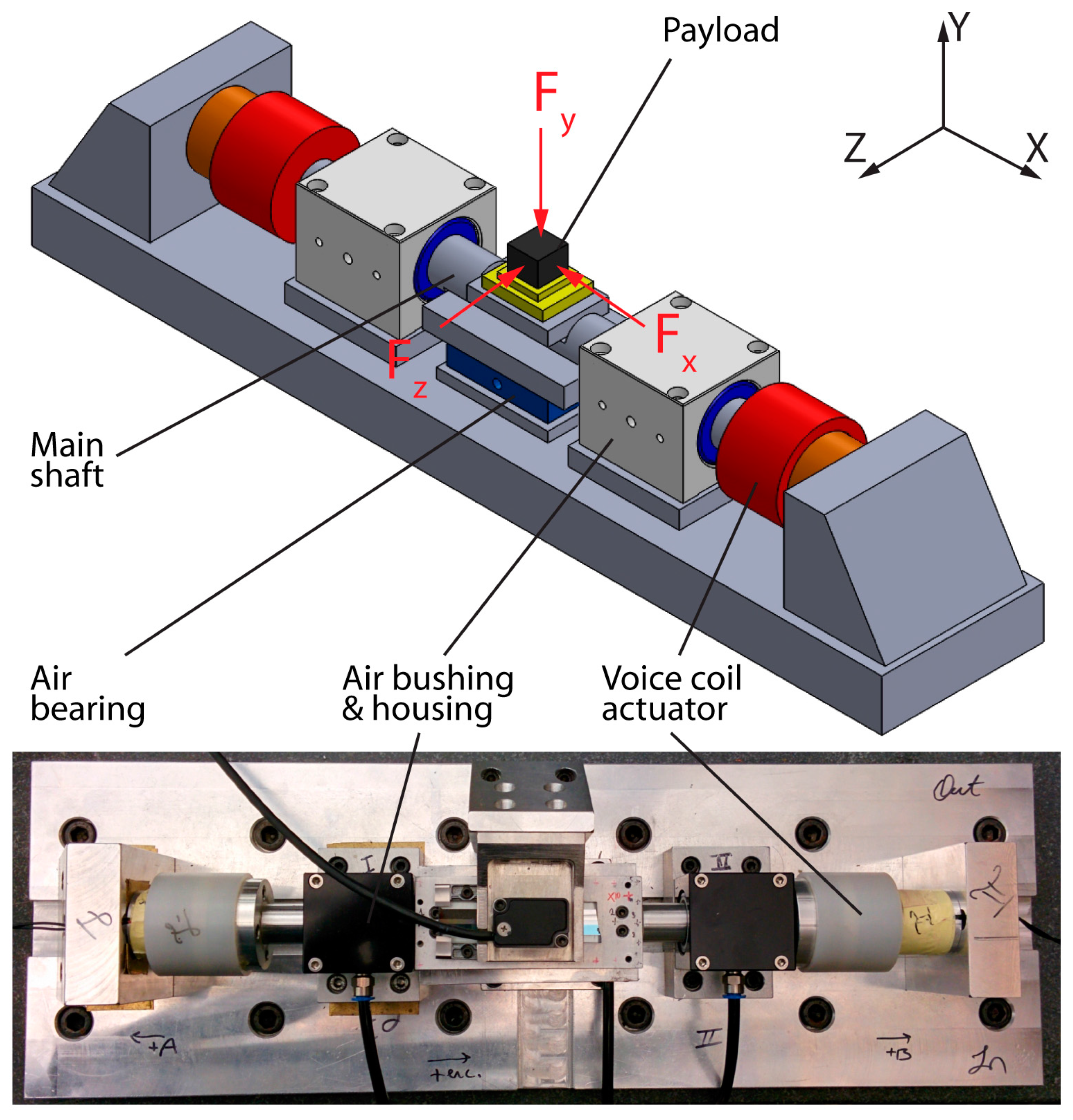
Figure 2.
Air-bushing/bearing arrangement of the motion stage.

Figure 3.
Coarse approximation for air bearing rotational stiffness.
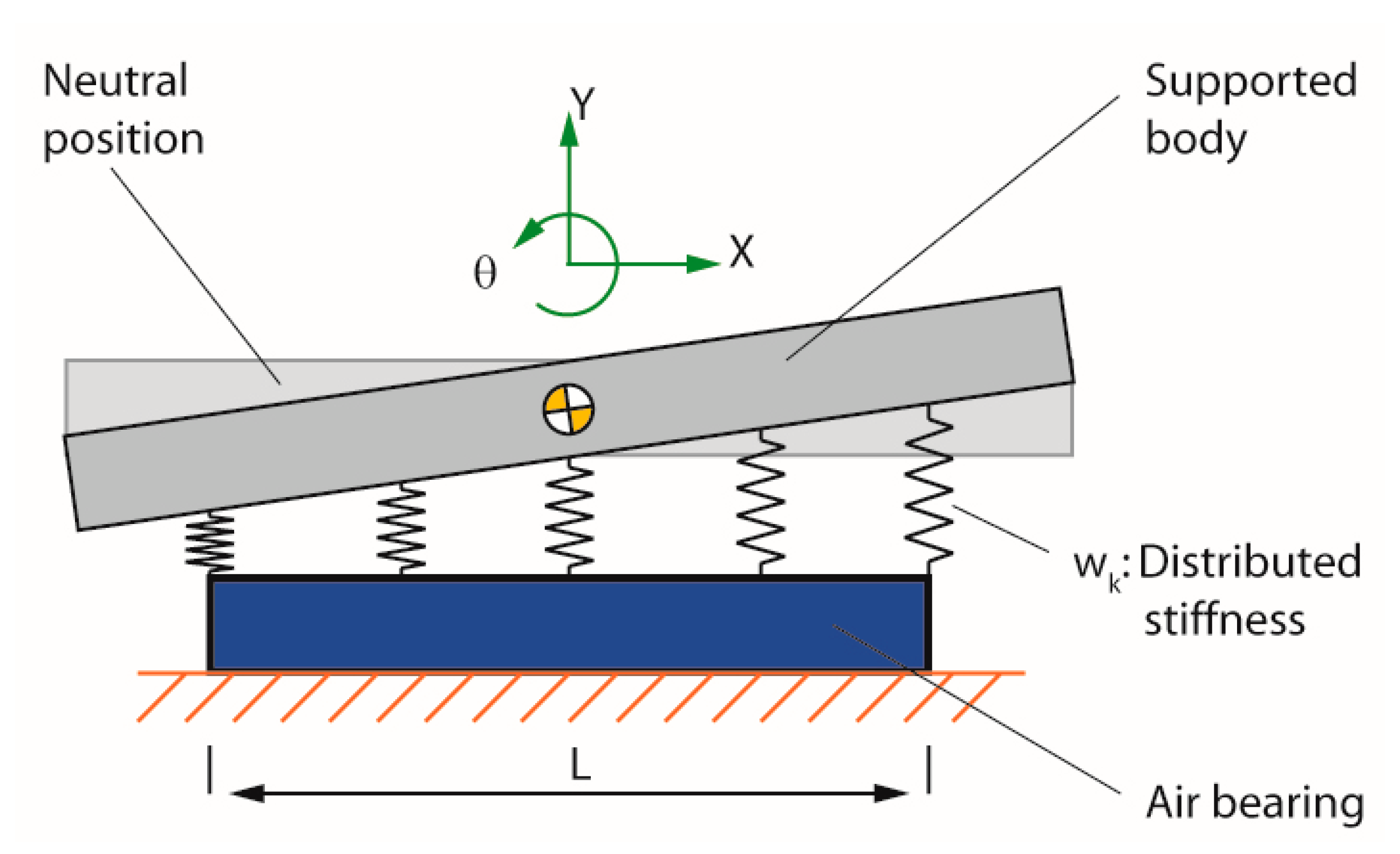
Figure 4.
Impact and measurement locations for method 1 (modified peak-picking).
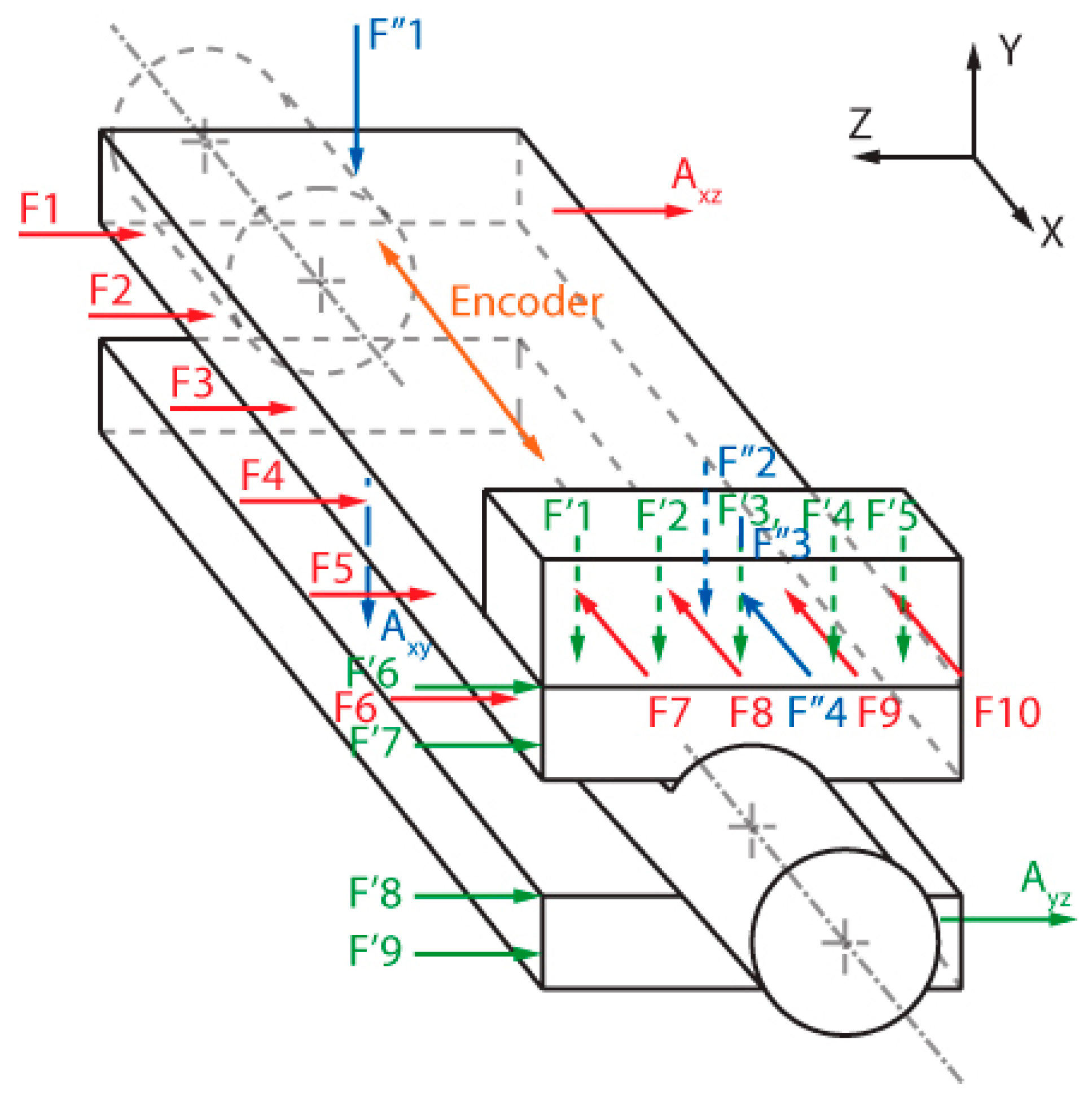
Figure 5.
Real and imaginary part plots of accelerance and receptance of a sample FRF.
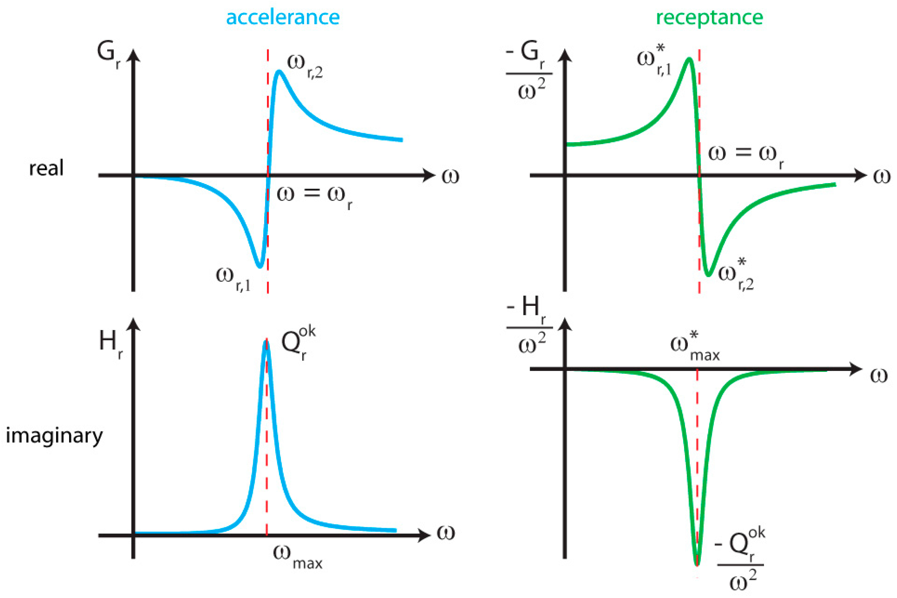
Figure 6.
Comparison of using different peak-picking formulations: (a) Damping ratio estimation; (b) Natural frequency estimation.
Figure 6.
Comparison of using different peak-picking formulations: (a) Damping ratio estimation; (b) Natural frequency estimation.
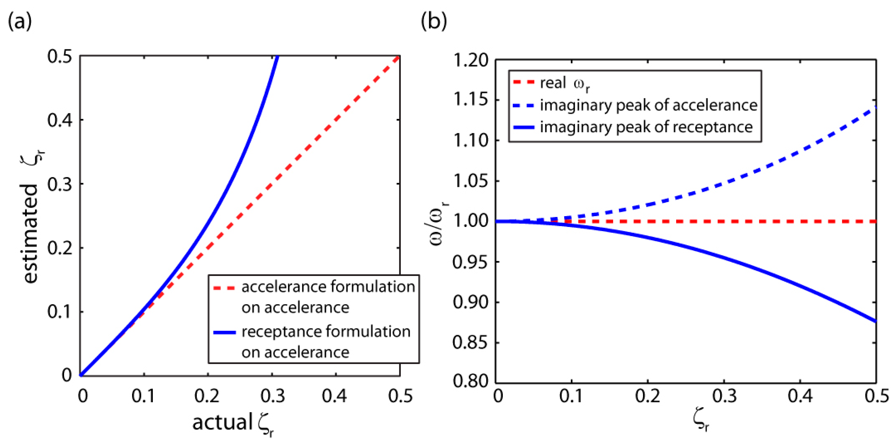
Figure 7.
Using the imaginary peak/dip values to determine the modal displacements.
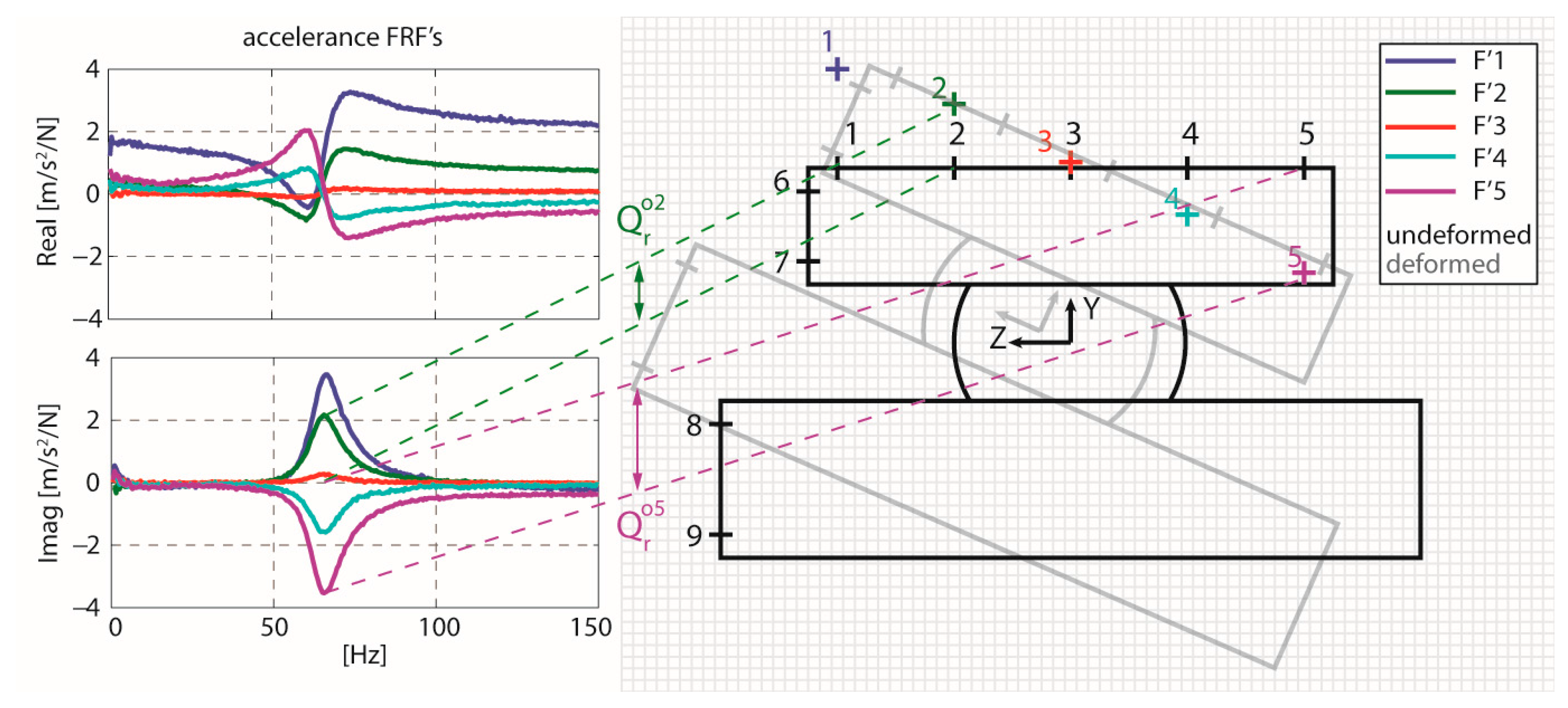
Figure 8.
Experimental procedure for method 2: (a) Photograph of the impact hammer and the tri-axis accelerometer at the A4 position; (b) Impact and measurement points.
Figure 8.
Experimental procedure for method 2: (a) Photograph of the impact hammer and the tri-axis accelerometer at the A4 position; (b) Impact and measurement points.
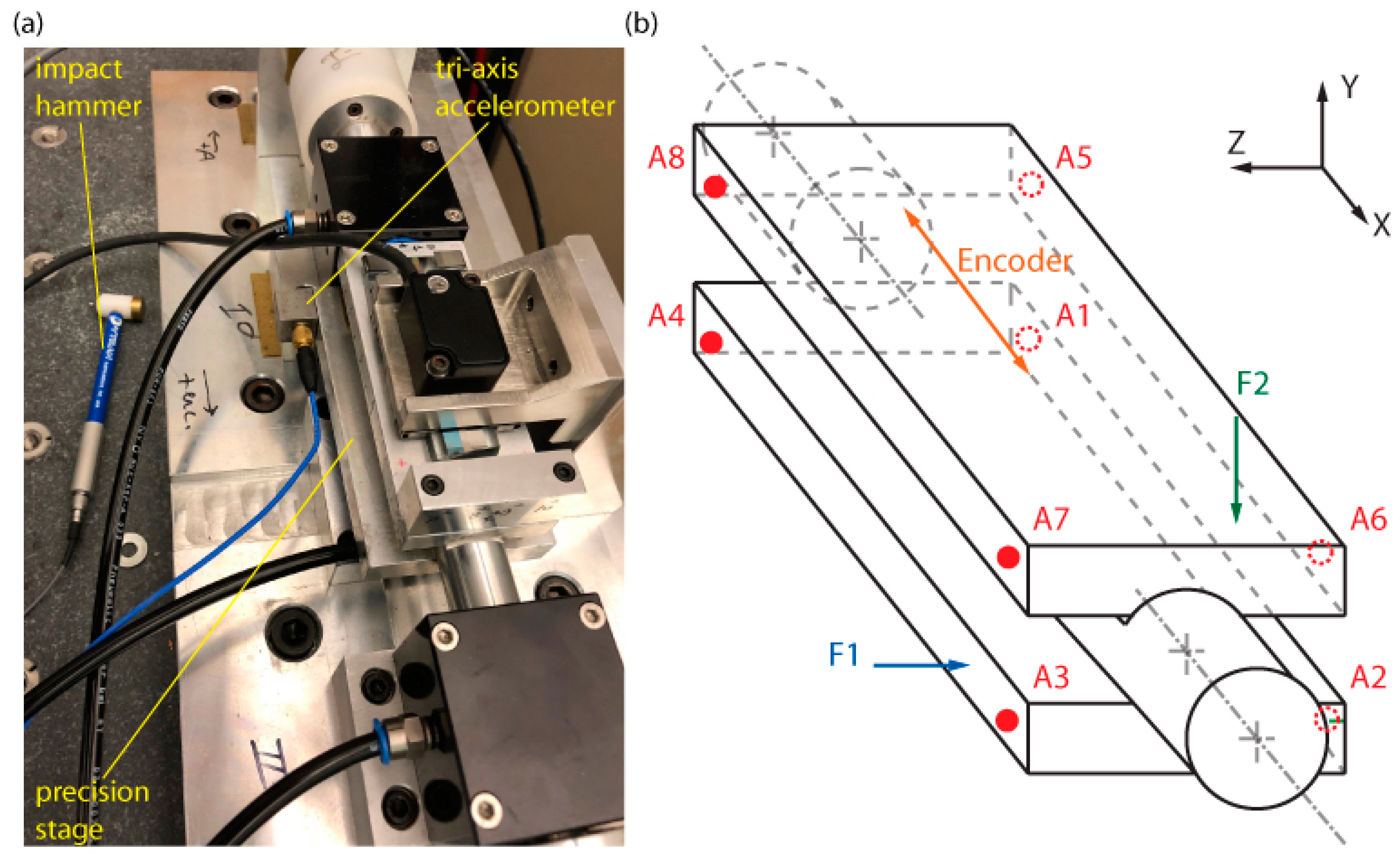
Figure 9.
Comparative modal testing results from the two methods and predictions at the design phase. Dimensions in mm.
Figure 9.
Comparative modal testing results from the two methods and predictions at the design phase. Dimensions in mm.
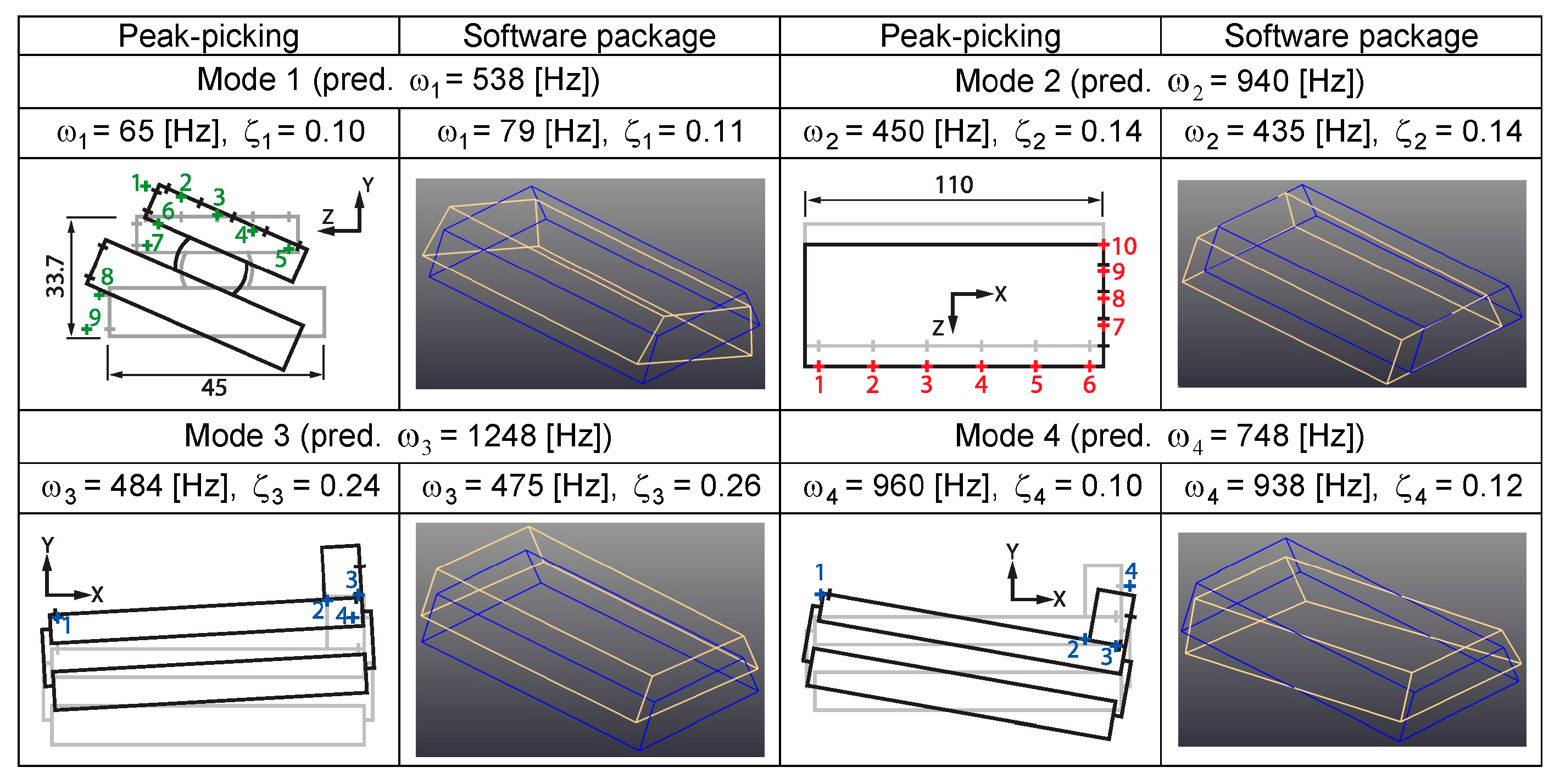
Figure 10.
Machine tool coordinate system and error motions (copied by Waterloo University with the permission of the Standards Council of Canada (SCC) on behalf of ISO) [20].
Figure 10.
Machine tool coordinate system and error motions (copied by Waterloo University with the permission of the Standards Council of Canada (SCC) on behalf of ISO) [20].
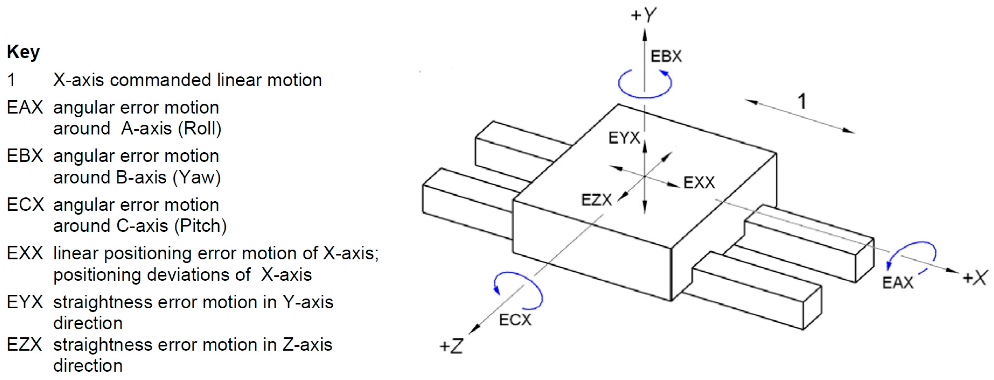
Figure 11.
Locations of the measurement optics with respect to the center of gravity: (a) Retroreflector; (b) Wollaston prism. Dimensions in mm.
Figure 11.
Locations of the measurement optics with respect to the center of gravity: (a) Retroreflector; (b) Wollaston prism. Dimensions in mm.
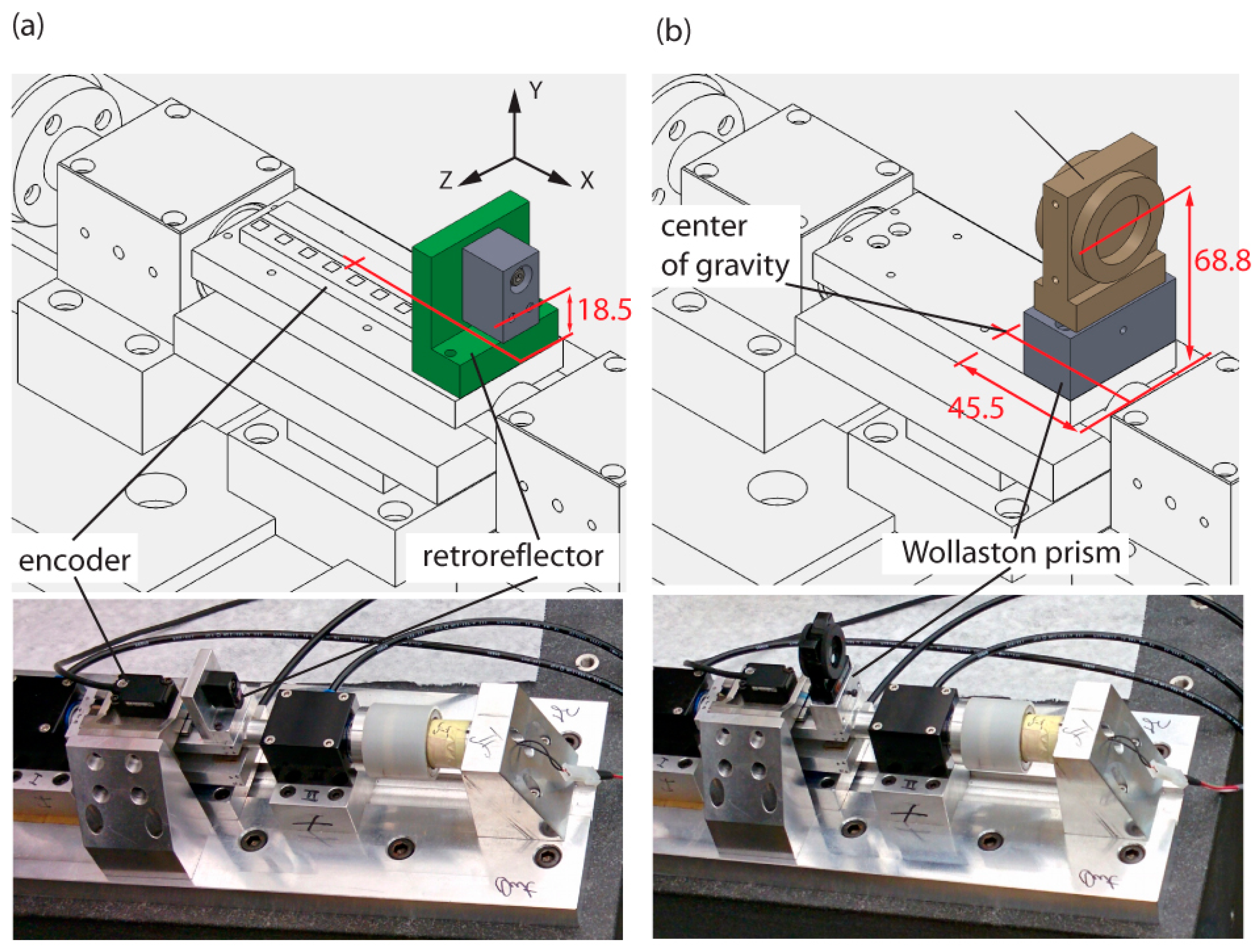
Figure 12.
EXX results: (a) Raw measurement; (b) Abbe compensated with straight line fit; (c) ISO presentation after slope removal.
Figure 12.
EXX results: (a) Raw measurement; (b) Abbe compensated with straight line fit; (c) ISO presentation after slope removal.
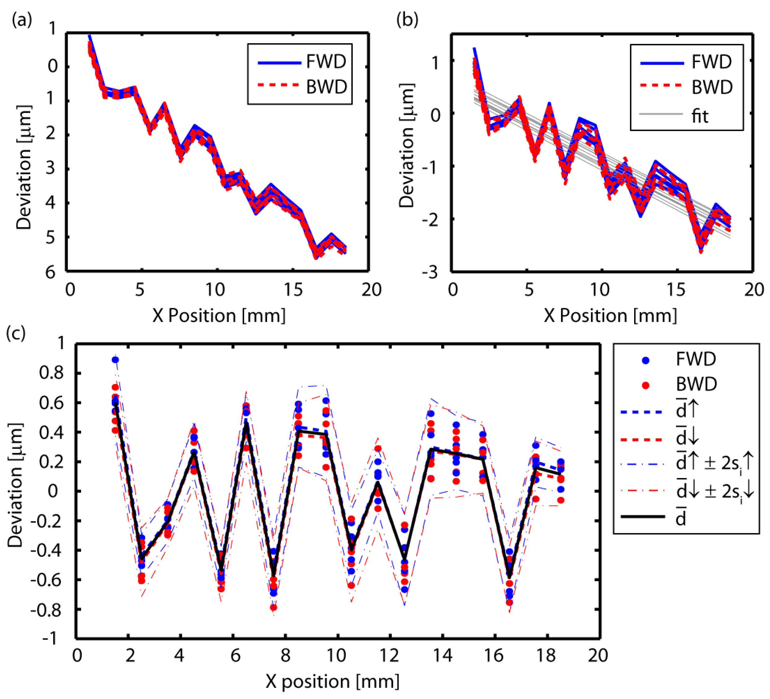
Figure 13.
EYX results: (a) Raw measurement; (b) Abbe compensated with straight line fit; (c) ISO presentation after slope removal.
Figure 13.
EYX results: (a) Raw measurement; (b) Abbe compensated with straight line fit; (c) ISO presentation after slope removal.
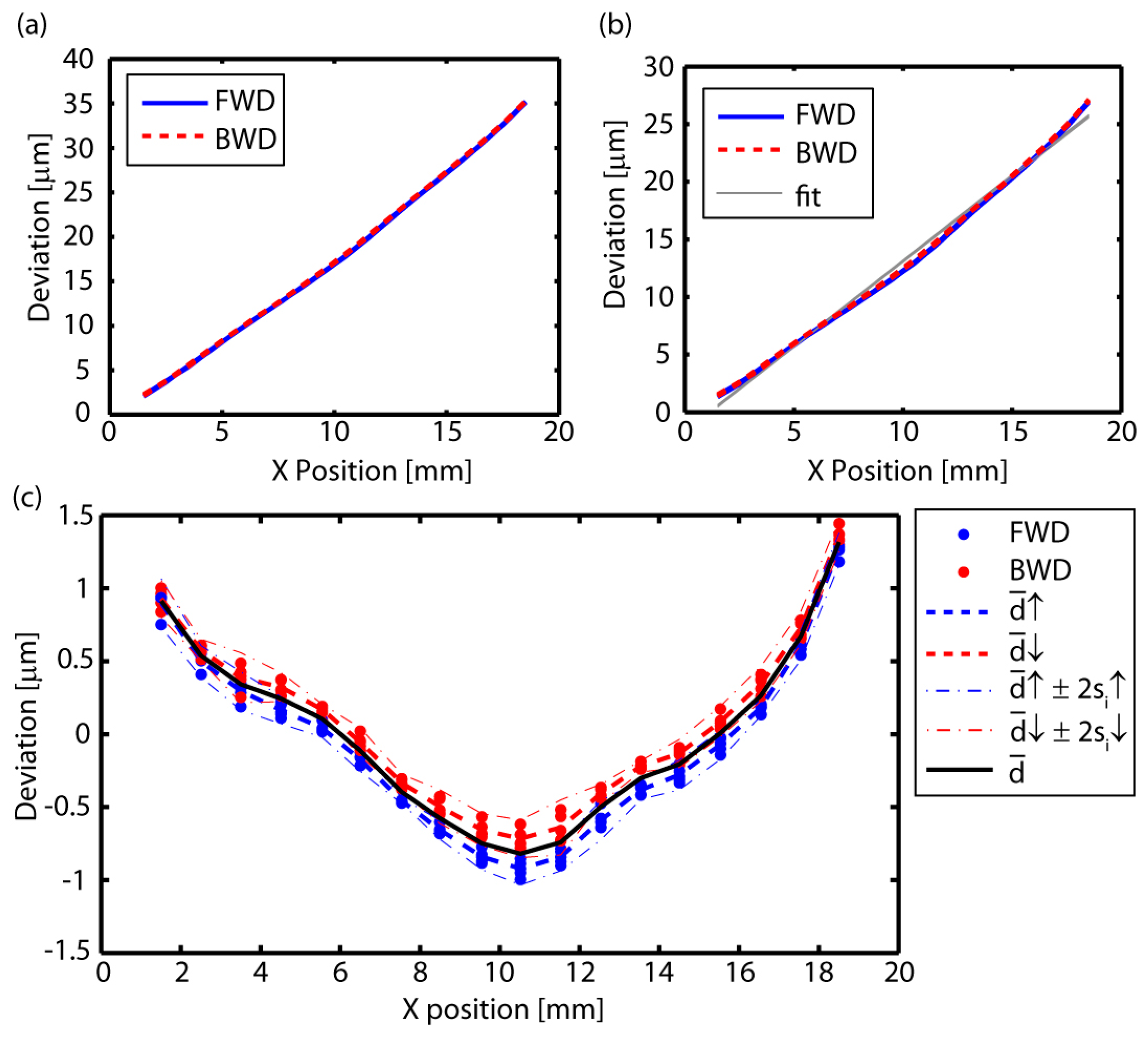
Figure 14.
EZX results: (a) Raw measurement; (b) Abbe compensated with straight line fit; (c) ISO presentation after slope removal.
Figure 14.
EZX results: (a) Raw measurement; (b) Abbe compensated with straight line fit; (c) ISO presentation after slope removal.
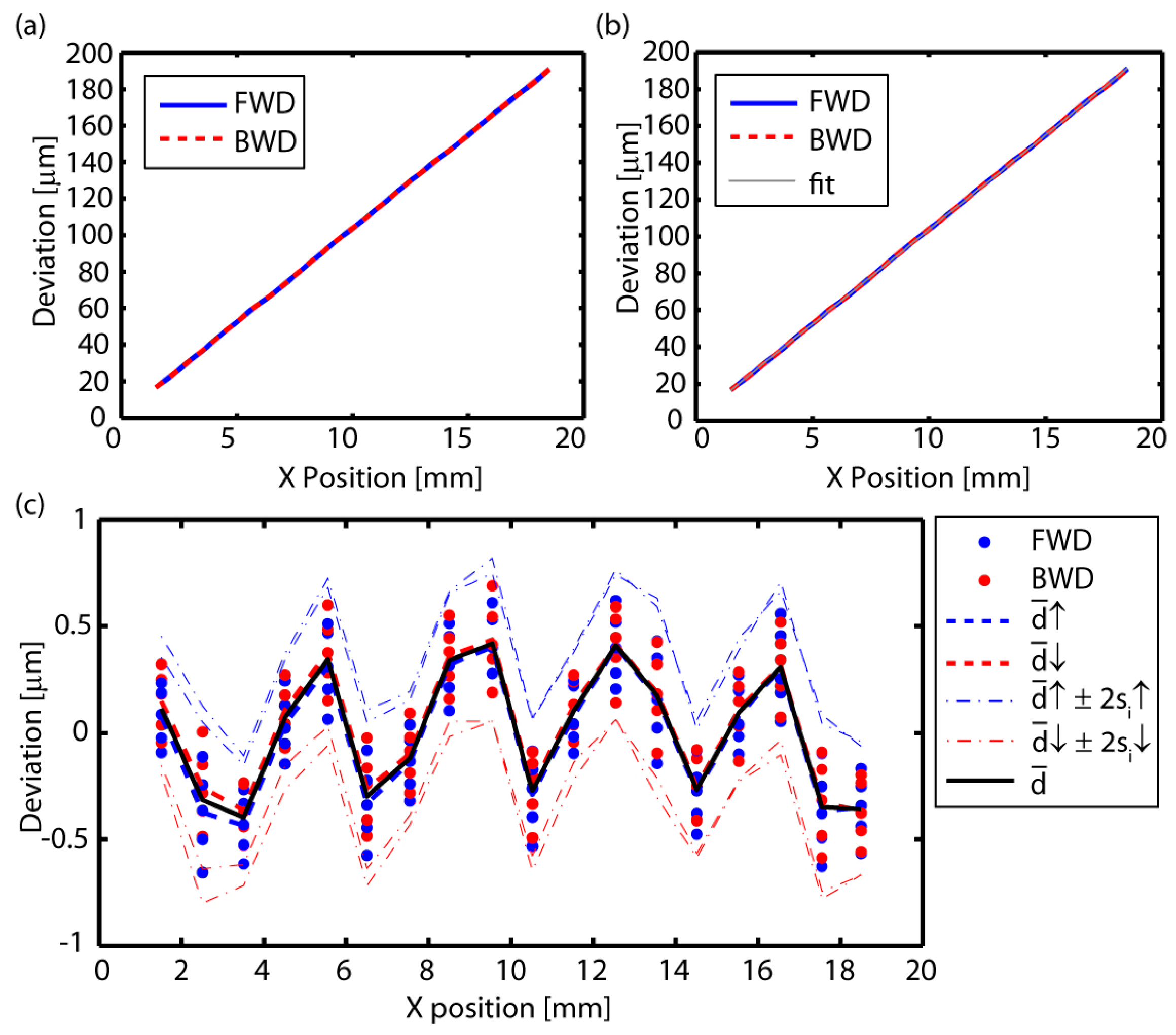
Figure 15.
EBX results in ISO presentation.

Figure 16.
ECX results in ISO presentation.
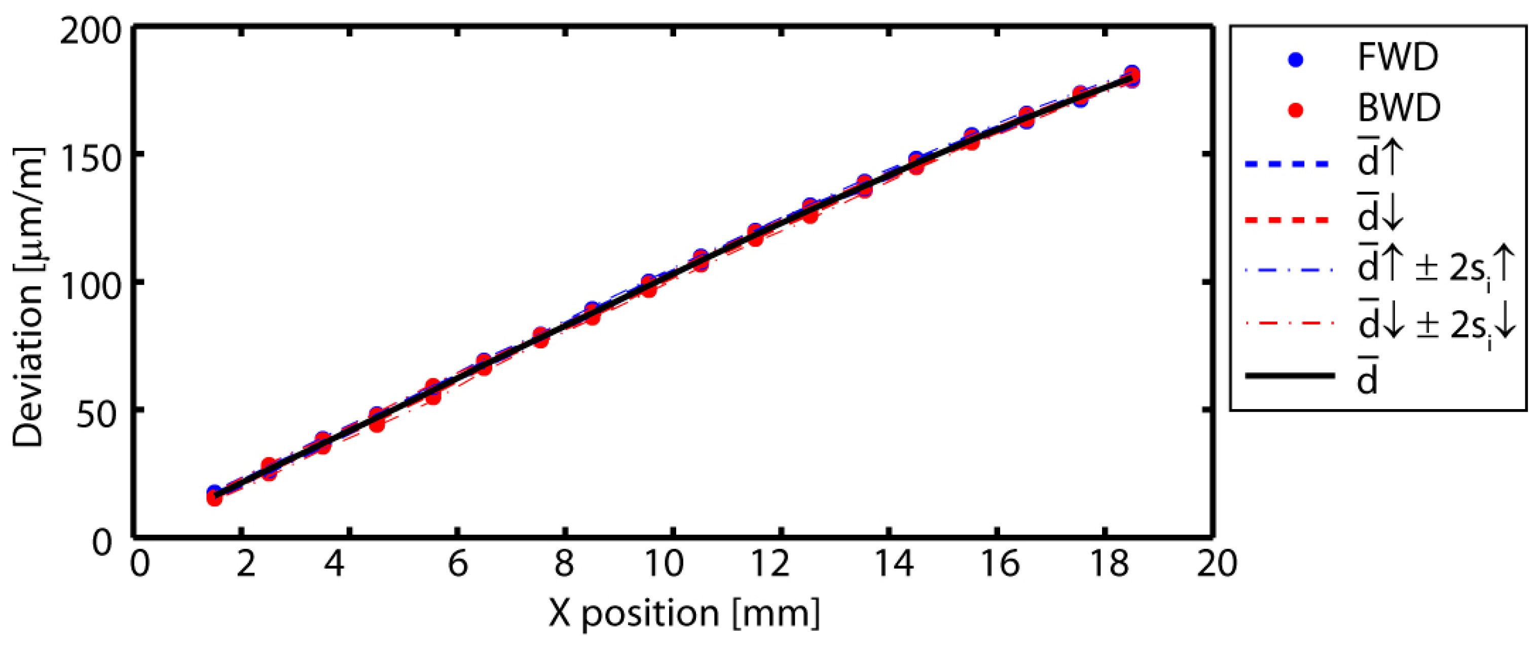
Figure 17.
Tolerances on the main shaft.
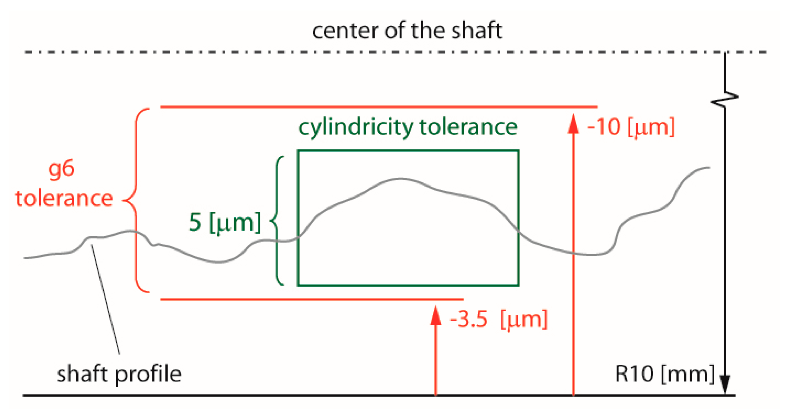
Figure 18.
Diagram of the stage with key variables relevant to thermal disturbance sensitivities. Dimensions in mm.
Figure 18.
Diagram of the stage with key variables relevant to thermal disturbance sensitivities. Dimensions in mm.
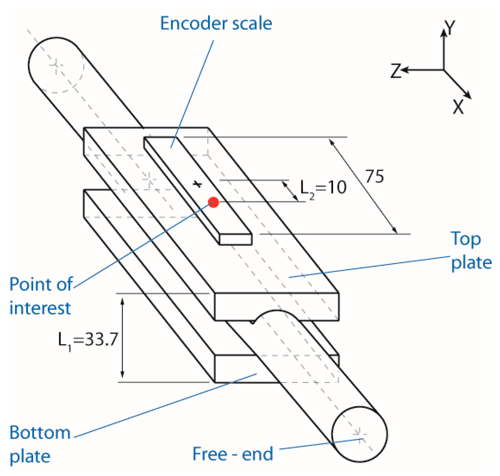
Figure 19.
Temperature readings over 8 hours of continuous operation.
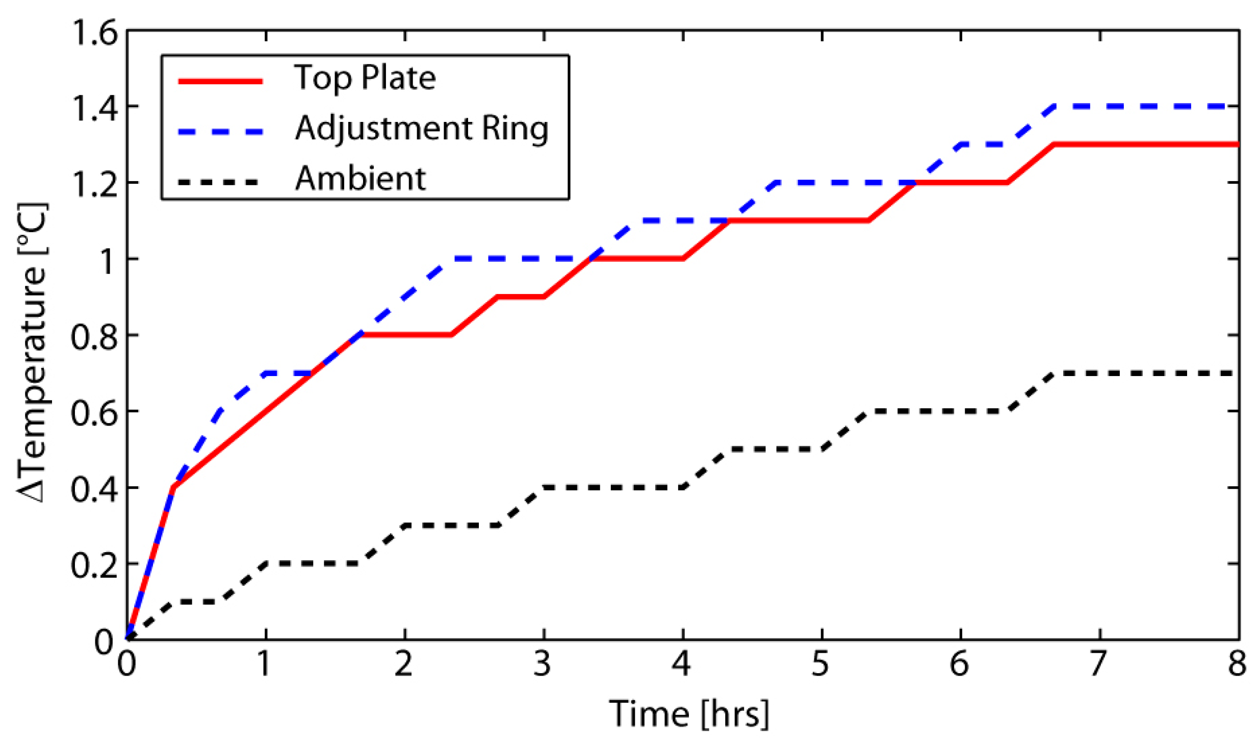
Figure 20.
Control block diagram with the machining force disturbance.
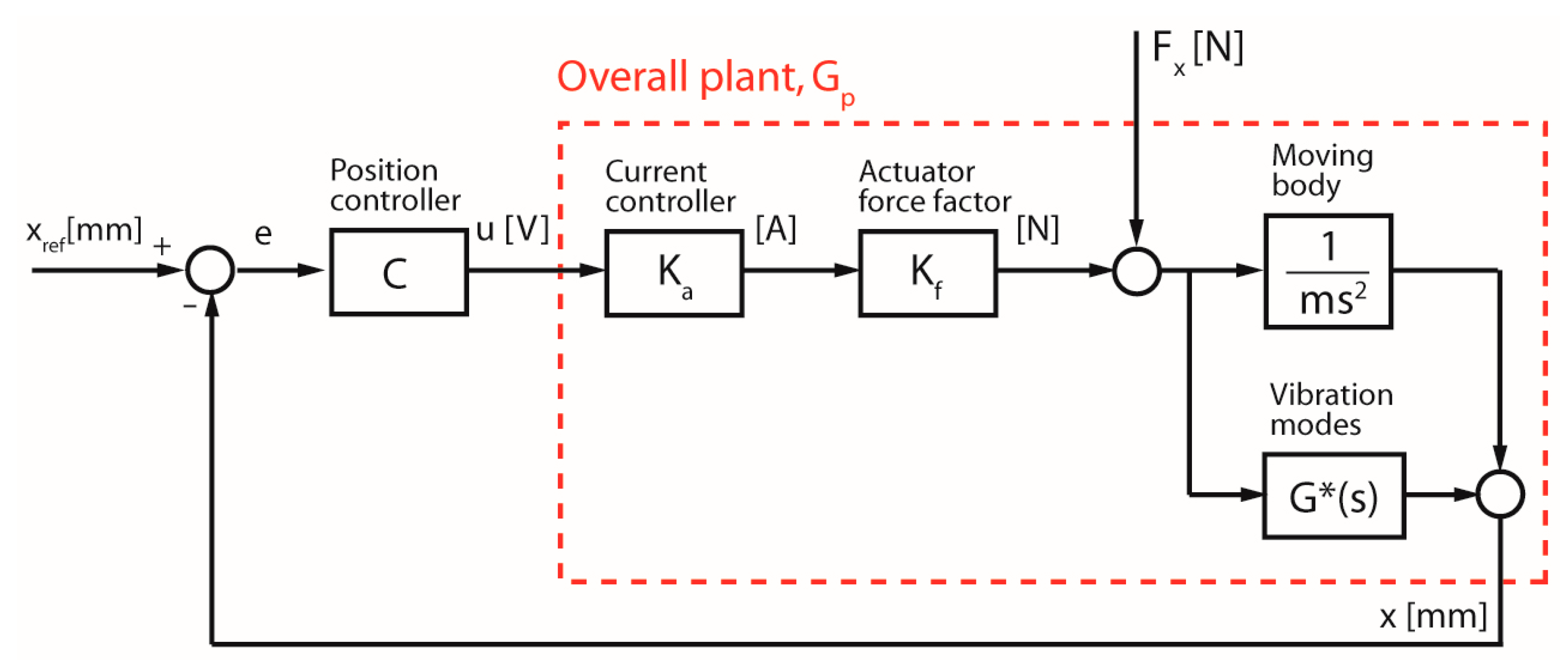
Figure 21.
Frequency domain functions: (a–c) Transfer function between forces and deflections in the X-, Y-, Z-directions; (d) Total deflection as a function of frequency.
Figure 21.
Frequency domain functions: (a–c) Transfer function between forces and deflections in the X-, Y-, Z-directions; (d) Total deflection as a function of frequency.

Table 1.
Air-bushing/bearing stiffness properties and dimensions.
| Property | Symbol | Value |
|---|---|---|
| Air bushing axial stiffness | 23 N/μm | |
| Air bushing rotational stiffness | 2.8 Nm/mrad | |
| Air bearing axial stiffness | 35 N/μm | |
| Air bearing roll stiffness (estimated) | 4.7 Nm/mrad | |
| Air bearing pitch stiffness (estimated) | 7.3 Nm/mrad | |
| Air bearing length along the X-axis | 50 mm | |
| Air bearing length along the Z-axis | 40 mm | |
| Distance between the middle of the air bushings along the X-axis | 180 mm |
Table 2.
Inertia properties of the moving body.
| Property | Symbol | Value |
|---|---|---|
| Mass | 1.318 kg | |
| Moment of inertia in A (Roll) | 409 kg mm2 | |
| Moment of inertia in B (Yaw) | 17,439 kg mm2 | |
| Moment of inertia in C (Pitch) | 17,454 kg mm2 |
Table 3.
Prediction of the natural frequencies.
| Direction | Expression | Natural Frequency (Hz) |
|---|---|---|
| Y (Vertical) | 1248 | |
| Z (Horizontal) | 940 | |
| A (Roll) | 538 | |
| B (Yaw) | 741 | |
| C (Pitch) | 748 |
Table 4.
Comparison of the two independent methods used in modal testing.
| Feature | Method 1 (Modified Peak-Picking) | Method 2 (Software Package) |
|---|---|---|
| Frequency response function (FRF) acquisition system | CutPRO® MalTF module by Manufacturing Automation Laboratory (MAL), Inc. | LMS Test.Lab® by Siemens-PLM Software |
| Testing procedure | Roving hammer | Roving accelerometer |
| Accelerometer type | Dytran® 3035AG (1-channel) | PCB Electronics® 356A02 (3-channel) |
| Impact hammer type | Dytran® 5800SL | Dytran® 5800SL |
| Identification of the natural frequency and damping ratio | Modified peak-picking method | PolyMAX [18] |
| Identification of the mode shape vectors | Modified peak-picking method | Least-Squares Frequency Domain (LSFD) [19] |
| Presentation of the mode shapes | Manual 2D drawings | Automated 3D animations |
Table 5.
Target positions used in error measurements.
| i | (mm) | i | (mm) | i | (mm) |
|---|---|---|---|---|---|
| 1 | 1.509 | 7 | 7.548 | 13 | 13.545 |
| 2 | 2.508 | 8 | 8.501 | 14 | 14.509 |
| 3 | 3.507 | 9 | 9.549 | 15 | 15.533 |
| 4 | 4.510 | 10 | 10.515 | 16 | 16.547 |
| 5 | 5.548 | 11 | 11.526 | 17 | 17.549 |
| 6 | 6.501 | 12 | 12.543 | 18 | 18.505 |
Table 6.
Error motion parameters [21].
Table 6.
Error motion parameters [21].
| Parameter | Definition | Formula |
|---|---|---|
| Reversal value | , | |
| Mean reversal value | ||
| Range mean bidirectional positional deviation | ||
| Systematic positional deviation | ||
| Repeatability of positioning | , , , | |
| Accuracy | − |
Table 7.
Linear accuracies.
| EXX (Linear) | EYX (Vertical) | EZX (Horizontal) | |||||||
|---|---|---|---|---|---|---|---|---|---|
| (μm) | bi | bi | bi | ||||||
| N/A | N/A | 0.1 | N/A | N/A | 0.2 | N/A | N/A | 0.1 | |
| N/A | N/A | 0.0 | N/A | N/A | 0.1 | N/A | N/A | 0.0 | |
| N/A | N/A | 1.2 | N/A | N/A | 2.1 | N/A | N/A | 0.8 | |
| 1.2 | 1.2 | 1.2 | 2.1 | 2.2 | 2.3 | 0.8 | 0.8 | 0.9 | |
| 0.7 | 0.7 | 0.7 | 0.4 | 0.3 | 0.5 | 0.8 | 0.9 | 0.9 | |
| 1.6 | 1.7 | 1.8 | 2.3 | 2.4 | 2.5 | 1.6 | 1.5 | 1.6 | |
Table 8.
Angular accuracies.
| EBX (Yaw) | ECX (Pitch) | |||||
|---|---|---|---|---|---|---|
| (μm/m) | bi | bi | ||||
| N/A | N/A | 0.7 | NA | NA | 2.0 | |
| N/A | N/A | 0.0 | NA | NA | −1.0 | |
| N/A | N/A | 4.5 | NA | NA | 163.4 | |
| 4.4 | 4.5 | 4.5 | 163.7 | 163.2 | 163.8 | |
| 3.2 | 3.4 | 3.4 | 6.6 | 4.5 | 6.6 | |
| 6.6 | 7.2 | 7.2 | 167.0 | 167.2 | 167.5 | |
Table 9.
Predicted error budget.
| Error Components | PV Magnitude (nm) |
|---|---|
| Position sensor resolution () | 0.97 |
| Position sensor grating error () | 2000 |
| Y straightness () | 2500 |
| Z straightness () | 2500 |
| Arithmetic sum | 7001 |
| RMS sum | 1173 |
| Mean | 4087 |
Table 10.
Summary of geometric accuracies.
| Component | Accuracy (A) | Repeatability (R) | Units |
|---|---|---|---|
| EXX | 1.8 | 0.7 | (µm) |
| EYX | 2.5 | 0.5 | (µm) |
| EZX | 1.6 | 0.9 | (µm) |
| EBX | 7.2 | 3.4 | (µm/m) |
| ECX | 167.5 | 6.6 | (µm/m) |
Table 11.
Thermal sensitivities and parameters used in calculations.
| Quantity | Symbol | Value |
|---|---|---|
| Thermal coefficient of expansion of Aluminum 6061 | 23.5 ppm/K | |
| Thermal coefficient of expansion of the glass encoder scale | 8 ppm/K | |
| Thickness of the moving body | 33.7 mm | |
| Distance between the center of the top plate and the encoder scale | 10 mm | |
| Thermal sensitivity along the X-axis | 235 nm/K | |
| Thermal sensitivity along the Y-axis | 396 nm/K | |
| Total thermal sensitivity | 460 nm/K |
Table 12.
The error budget.
| PV Magnitude (nm) | |||
|---|---|---|---|
| Repeatable Errors Conserved | Repeatable Errors Subtracted | Estimated at Design Phase | |
| Linear (EXX) | 3964 | 675 | 2001 |
| Straightness | |||
| Vertical (EYX) | 2503 | 486 | 2500 |
| Horizontal (EZX) | 1620 | 936 | 2500 |
| Angular | (included in Linear) | - | |
| Servo | 30 | 30 | - |
| Thermal | 92 | 92 | - |
| Machining force | 1748 | 1748 | |
| Total Error | |||
| Arithmetic Sum | 9957 | 3967 | 7001 |
| RMS Sum | 1518 | 621 | 1173 |
| Mean | 5738 | 2294 | 4087 |
© 2018 by the authors. Licensee MDPI, Basel, Switzerland. This article is an open access article distributed under the terms and conditions of the Creative Commons Attribution (CC BY) license (http://creativecommons.org/licenses/by/4.0/).
Share and Cite
MDPI and ACS Style
Okyay, A.; Erkorkmaz, K.; Khamesee, M.B. Modal Analysis, Metrology, and Error Budgeting of a Precision Motion Stage. J. Manuf. Mater. Process. 2018, 2, 8. https://doi.org/10.3390/jmmp2010008
AMA Style
Okyay A, Erkorkmaz K, Khamesee MB. Modal Analysis, Metrology, and Error Budgeting of a Precision Motion Stage. Journal of Manufacturing and Materials Processing. 2018; 2(1):8. https://doi.org/10.3390/jmmp2010008
Chicago/Turabian StyleOkyay, Ahmet, Kaan Erkorkmaz, and Mir Behrad Khamesee. 2018. "Modal Analysis, Metrology, and Error Budgeting of a Precision Motion Stage" Journal of Manufacturing and Materials Processing 2, no. 1: 8. https://doi.org/10.3390/jmmp2010008