Online Tool Wear Classification during Dry Machining Using Real Time Cutting Force Measurements and a CNN Approach

Abstract

The new generation of ICT solutions applied to the monitoring, adaptation, simulation and optimisation of factories are key enabling technologies for a new level of manufacturing capability and adaptability in the context of Industry 4.0. Given the advances in sensor technologies, factories, as well as machine tools can now be sensorised, and the vast amount of data generated can be exploited by intelligent information processing techniques such as machine learning. This paper presents an online tool wear classification system built in terms of a monitoring infrastructure, dedicated to perform dry milling on steel while capturing force signals, and a computing architecture, assembled for the assessment of the flank wear based on deep learning. In particular, this approach demonstrates that a big data analytics method for classification applied to large volumes of continuously-acquired force signals generated at high speed during milling responds sufficiently well when used as an indicator of the different stages of tool wear. This research presents the design, development and deployment of the system components and an overall evaluation that involves machining experiments, data collection, training and validation, which, as a whole, has shown an accuracy of 78%.

1. Introduction

Industry 4.0 aims at leveraging manufacturing systems to the level where the right combination of advanced information and communication technologies (ICT) and manufacturing enables the implementation of flexible, smart and reconfigurable manufacturing processes [1,2]. The adoption of smart manufacturing lays out a novel industrial paradigm where elements of artificial intelligence, monitoring equipment and big data technologies intertwine together to provide learning, reasoning and decision making support, hence playing a crucial role in minimising operators’ involvement [3,4]. In other words, smart manufacturing is defined as the utilisation of advanced data analytics that, when applied to large volumes of rapidly generated manufacturing data, significantly increases production efficiency, enhances processes flexibility and improves product performance. This data-driven manufacturing has been characterised by enabling customer-centric product development, self-organisation, self-execution, self-regularisation, as well as self-learning and self-adaptation [5]. In particular, the latest is performed by exploiting both historical and real-time generated data to realise proactive maintenance and quality control. For instance, in predicted condition-based maintenance [6], faults can be diagnosed and, consequently, prevented by looking at past, current, as well as expected operational traits of the manufacturing system. Therefore, shedding light on performance indicators such as the remaining useful life of degrading equipment would, in turn, allow one to adapt a manufacturing system proactively to cope with potential production errors and decrease disruptions.

Machine learning (ML) algorithms have proven successful in detecting patterns, gaining insight and building predictive models using large volumes of manufacturing data. Although ML faces critical scalability challenges to unleash the hidden value of big data, it thrives when presented with large datasets and powerful computing environments [7], hence making them instrumental for the implementation of condition-based maintenance based on system performance indicators. This work focuses on tool wear assessment, which is characterised by the gradual loss of the ideal cutting tool edge geometry due to the developed cutting forces and temperatures, as well as the kinematics of the cutting process [8]. In production, quantifying the remaining useful life of a tool is important, as it is highly correlated with product quality measurements such as the surface finish of the workpiece. Depending on the cutting conditions and purpose of the workpiece, finding the right moment for replacing a tool is challenging as this usually happens either too late or too soon. In the former, tools can present signs of wear earlier than expected, therefore requiring prompt replacement before affecting the quality of the manufactured workpiece. In the latter, tools are replaced following manufacturing lifetime specifications, even when workpiece quality is satisfactory and tools are performing well, hence increasing the number of disruptions and production loss. Therefore, this paper presents the design, development, deployment and validation of an online tool wear classification system that fits within the area of control monitoring systems and predicted condition-based maintenance. In particular, it enlarges a methodology for the online assessment of flank wear based on force signals’ classification using deep learning. This approach demonstrates that a big data analytics method for classification applied to a large volume of force signals generated at high speed during milling responds sufficiently well when used as an indicator of the different evolutionary stages of tool degradation. In the rest of this paper, related work and background are introduced in Section 2. Then, Section 3 enlarges the design, development and deployment of the system components at both the monitoring infrastructure and computing architecture level. Section 4 enlarges data engineering and other management aspects, whereas Section 5 describes the experiments, results and online validation of online tool wear classification using real-time force signals. Finally, Section 6 presents conclusions and future work.

2. Related Work

In machining, characterising and monitoring the degradation of tool edges is important since it plays a significant role in the machined parts’ quality, remaining tool life and machine downtime, hence affecting product yield and cost-saving productivity. Tool wear is related to many factors such as the mechanical stress, temperature and the use of coolant during the cutting process, so that it cannot be avoided and it is essential to characterise it, as well as to be able to monitor, foresee and control its progress. Thus, developing novel smart methodologies contributes to more informed and better decision making, which is reflected in cost-efficient industrial productivity, closes the gap towards unattended machining, increases machining time and reduces employee idle time. Most research works are divided into the characterisation of the wear itself and the monitoring of tool wear, which are related, but yet different concepts. The first one focuses on techniques for quantifying modifications of the cutting edge geometry, whereas the latter focuses on methodologies that report the progression of the wear by correlating machining information with a given wear characterisation. Since the focus of this paper is tool wear monitoring, the following subsections overview the most recent developments in the field.

2.1. Tool Wear Monitoring

Tool wear monitoring can be divided into direct and indirect methods. In the former, the actual value of a wear parameter such as the flank, the rake or the crater is directly quantified by optical devices, geometrical assessment or measuring electrical resistance, to name a few. Tool condition monitoring is a vast field of research that has been carried out over several decades, and a good number of publications have been selected and featured in [9,10], paving the way for the exploration of better monitoring models. An example of a direct tool wear monitoring approach using computer vision and ML techniques has been reported in [11]. This work focused on the image characterisation for wear extraction on milling inserts. In particular, an accuracy of $88\%$ has been achieved with a support vector machine trained and tested with images taken from over fifty tools’ inserts and classes defined by experts of the field. Like most direct approaches, this has the advantage of high accuracy. However, it has to be conducted between cycles only, which makes it difficult to implement as an in-process technique. Moreover, it depends on many factors such as image resolution and recognition accuracy, which is usually hindered by the presence of fluid or the development of a built-up edge and requires image processing-specific knowledge such as using filters, applying rotations and cropping, all of which would be difficult to integrate in an automated system. In indirect tool wear monitoring, process parameters that correlate with wear are conducted using calibration procedures. Examples of this applied on dry machining have been reported in [12,13,14]. These approaches focus on capturing cutting forces, motor load signals or energy consumption in order to analyse how different cutting conditions and material characteristics relate to the wear of the tool. Although these approaches report successful results using specially-designed part geometries or materials with different hardness, they focus on problem-specific characterisations without delivering a scalable and extensible methodology; thus, being difficult to implement at the industrial level, lacking a smart methodology and, more importantly, failing to depict any possible online procedure. More advanced methods with a step closer to automation have been developed to improve the performance of tool condition monitoring. For instance, vibration combined with ML have been reported in [15,16]. These works focus on milling where acceleration signals are collected, filtered and more than ten statistical features extracted and identified. All this feature engineering working together with the characterisation of tool wear stages defined in terms of surface finishing were used for training an artificial neural network that achieved $95\%$ accuracy. A more sophisticated approach employing both Gaussian mixture hidden Markov models and back propagation neural networks was presented in [17], where a larger set of statistical features, 18 in total, and correlations have been extracted from force signals. Although these are elegant and robust data-driven methods, the preprocessing and identification of features are the main disadvantages, as these are time consuming and require expert knowledge. In addition, it is challenging to make approaches like these work online with real-time calibration procedures since they are not suitable for raw signals. Moreover, the scaling and extension of this approach to other types of machining or tools is not discussed. Currently, different ML methods are adopted more and more frequently to solve some of the identified issues.

2.2. Deep Learning in Condition Monitoring

Approaches based on signal processing that lead to feature extraction or dimensionality reduction are challenging to extend and generalise since they usually require domain expertise and prior knowledge, manual selection of features and expensive preprocessing, thus making them time consuming, inefficient and difficult to implement at the industrial level. These limitations become more evident when dealing with non-stationary, high frequency, large volumes of data coming from different sensors. Advanced machine learning methods such as autoencoders and back propagation neural networks have been proposed for the intelligent diagnosis of mechanical systems in industry and research [18,19] as these use data to construct models that can detect different conditions autonomously and are capable of learning valuable features from very large sets of raw data [20]. Others such as deep neural networks employ a hierarchical structure composed of multiple neural layers that, in a layer-by-layer fashion, extract intricate structures from large volumes of raw data and learn useful features across multiple levels of abstraction [21]. In particular, convolutional neural networks (CNN) [22] are one of the main models and have been very successful when applied to learn features autonomously by exploiting the spatial structure in raw data. For instance, with the aim of automatically learning features to detect faults on gearboxes, the work reported in [23] explored different CNN configurations applied to single-axis vibration data in the time, frequency and time-frequency domains. The results demonstrated that a CNN model is capable of ingesting raw data to undergo feature extraction, selection and classification, thus forming a feature learning system that outperforms traditional ML methods. Likewise, the comparison between traditional ML set up with feature engineering (i.e., features designed by experts) against a CNN model that learns from Fourier-transformed vibration signals of two accelerometers was reported in [24]. A lengthy review and experimental study of emerging research works on deep learning applied to machine health monitoring can be found in [25]. Inspired by the success of automated feature extraction from images [26], an enhanced approach for gearbox fault severity classification and anomaly detection was reported in [27]. In this case, vibration signals are converted by wavelet transform into time-frequency spectral images. which, together with different fault categories, serve as input to train and test a deep CNN in terms of sideband amplitudes with an accuracy of $99.5\%$. Another successful approach that combines acoustic emission sensor signals converted to time-frequency spectrograms for real-time monitoring of the workpiece quality with CNNs was reported in [28]. The application of a hybrid feature extraction method combined with CNNs for tool condition monitoring was reported in [29], where signals from the dynamometer and accelerometer were independently subject to time-frequency transformation using Morlet wavelet transform and feature extraction using PyWavelets. The output of these was then processed for the implementation of a CNN to model the complex relationship between the extracted features and the tool wear. In a further validation of this approach, signals from a current sensor were subject to healthy spectrum removal, which, with a number of statistical features, was used to identify and represent the fault within the signals. The achieved results were the highest when compared to Bayesian ridge regression, support vector machine and nearest neighbour. A tool condition monitoring system developed to report wear progression based on the flank wear and hardness variation was reported in [30]. The study focused on audible sound signals generated during end milling of alloy steel with hardness variation. The monitoring system was comprised of two functions to detect hardness changing of the workpiece and tool wear progression simultaneously. This involved sound collection of dry milling conducted with uncoated four-flute high-speed steel end mill tools within four wear levels, i.e., good, average, advanced and failure. Likewise, the workpiece was prepared with four levels of hardness so that when the tool cut different hardness, the generated sound signal captured by microphones would be associated with a specific hardness area. A total of 48 experimental runs generated 192 sound signals, which were subject to feature extraction using fast Fourier transform. Thus, the features labelled with associated tool wear level and hardness level together with signal samples of two different lengths were employed to build a CNN model. This approach has shown higher prediction accuracy when compared against a support vector machine, but a compatible result in the workpiece hardness monitoring. A bespoke deep learning model to address multiple space-based features from vibration signals in ultra-precision machining was introduced in [31]. In particular, the authors used vibration datasets obtained from shell machining for consumer electronics and claimed to avoid human-assisted feature identification. To achieve this, the vibration signals were preprocessed with fast Fourier and wavelet transforms to create a preliminary parallel training model that learned low-level features from the time, frequency and wavelet domains. This was implemented with multiple stacked sparse autoencoders in charge of extracting features from each domain without using labels. These extracted features were accommodated in an output array, which served as the input of another stacked sparse autoencoder, called the fusion model, that extracted higher level features. These were fed into a back propagation algorithm that learned to correlate the progression of the tool wear measured in terms of surface quality. The method was assessed using three different diamond cutting tools, four different tool wear types defined in terms of aluminium alloy surface finishing quality and 1625 raw vibration signals of 20 thousand data points each. The proposed method had an accuracy of $96.63\%$, which outperformed a back propagation neural network and a support vector machine.

The advance of ICT technologies together with a cost reduction of large computing power have encouraged the use of more robust and resilient cutting edge ML methods. In particular, deep learning combined with standard sensors and data acquisition equipment is a growing area in condition monitoring systems. However, the exploitation of these using big data for the development of end-to-end smart systems, without a signal analyst or image processing expertise, is starting to flourish. Although current deep learning solutions claim to have achieved high accuracy (a high percentage of correct classifications or low mean absolute error and root mean square error), it can be misleading to simply compare approaches based on these measures. Multiple layers of information processing modules in hierarchical structures will almost certainly provide an improved outcome [32]. The problem, however, is evaluating the computational effort of this processing. Most existing deep learning solutions use, for instance, Fourier and wavelet transforms or statistical feature extractions as the data pre-processing steps [25,33,34,35,36,37,38], and performing these computationally-expensive methods on real-time large datasets is not practical. Moreover, although these procedures reduce the training time required, they can introduce bias in the early training of an algorithm and lead to unreliable results. Nevertheless, it can be argued that performing feature extraction is against the philosophy of deep learning [32]. Therefore, this paper underlines an approach based on a very simple mathematical model that converts raw force signals into two-dimensional images that, when used as input to a standard CNN architecture, exploits internal spatial structures encoding edge devastation for reporting tool wear progression during dry machining on steel. In particular, the image encoding step does not need to process the complete dataset to provide an input to the CNN, nor modify the information content of the acquired signals, hence using the power of deep learning to extract relevant features from encoded samples of raw data. To our knowledge, the approach proposed here is the first one that truly provides a scalable online solution, as it works with raw data, is blind to the problem domain and has the potential to be easily applied to other condition monitoring problems.

3. Cutting Force Measurement during Dry Machining

The online tool wear classification system consists of a condition monitoring infrastructure and a software architecture. The condition monitoring infrastructure comprises all machining elements to perform steel milling with a milling cutter while monitoring and collecting force signals. The computing architecture involves those elements of software employed to collect and process data, classify and report the tool wear progress to the end user.

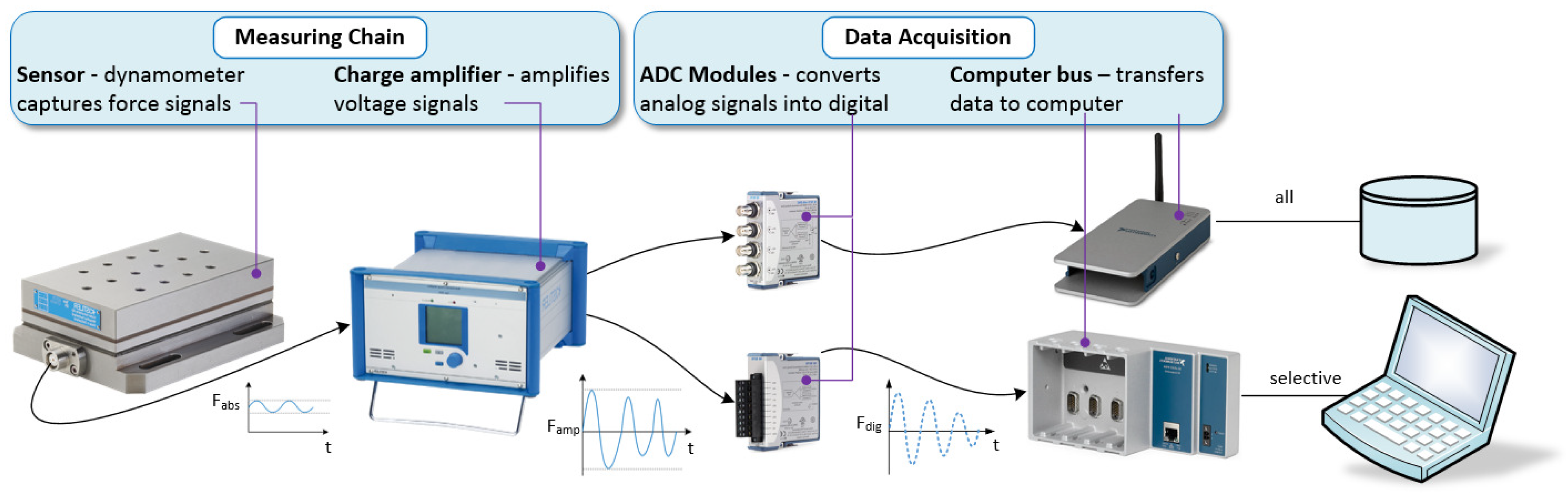
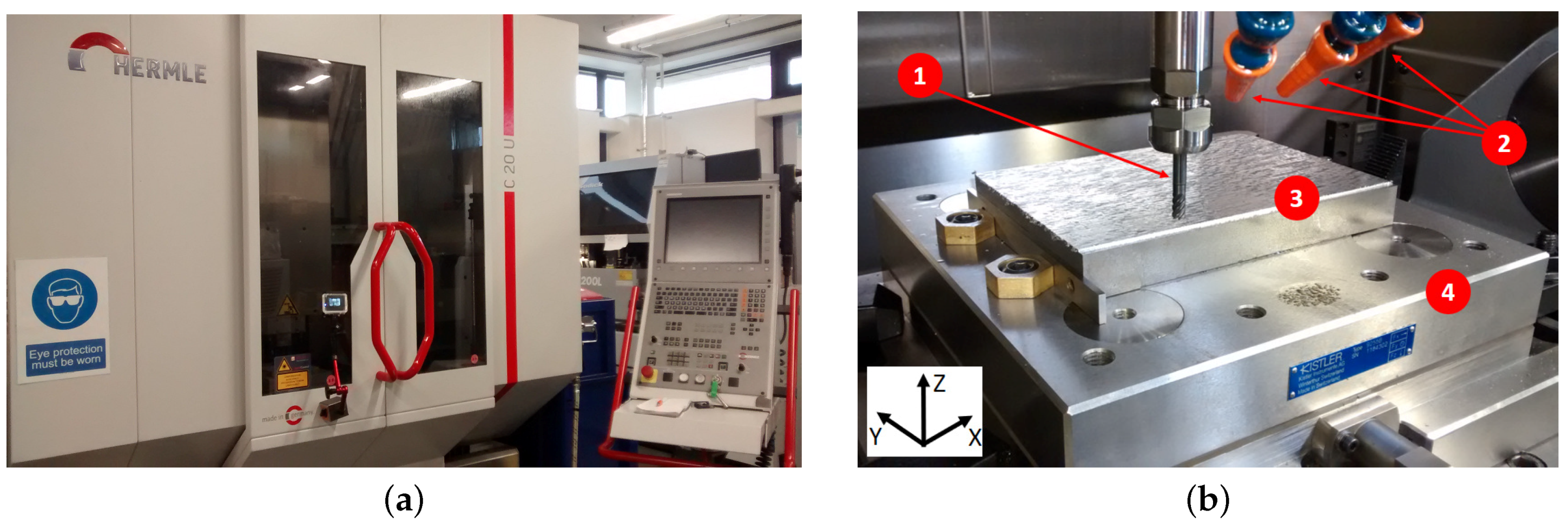
3.1. Condition Monitoring Infrastructure

The condition monitoring infrastructure consists of a measuring chain and a data acquisition system, as depicted in Figure 1. The former comprises a piezoelectric three-component dynamometer that measures the three orthogonal components of the cutting force, i.e., force values on the x-axis, y-axis and z-axis. The output of this dynamometer is connected to a four-channel charge amplifier that captures, amplifies and transmits the force signals to a dual data acquisition system. The latter is configured with two independent dynamic signal acquisition modules that condition and digitise the analogue signal from the charge amplifier before making it available throughout Ethernet-based computer bus devices. Thus, the output values of one computer bus device are captured in full and stored externally for offline analytics, whereas the output values of the other computer bus device are selectively captured and fed into the tool wear classification system.

For the specific purpose of this work, a vertical machining centre has been equipped with solid carbide end milling cutters to machine bright drawn mild steel (BDMS) workpieces. In particular, the milling machine was a Hermle C20U CNC programmed via its Heidenhain iTNC 530 control (see Figure 2a) to face mill a level surface line-by-line, i.e., an entire layer of material, with retraction and step over at the positioning feed rate along the x-axis. For all experiments, this CNC machine was fitted with two-flute cutters of $6\mathrm{mm}$, BDMS blocks of $180\times 125\times 25{\mathrm{mm}}^3$ and compressed air for dry machining, as depicted in Figure 2b. Considering the cutting parameters recommended by the cutting tool manufacturer, based on the workpiece material and for finishing operations, the milling parameters were fixed to $S=4775$ RPM, $f=287\mathrm{mm}/\min$, $a_e=2.7\mathrm{mm}$ and $a_p=0.3\mathrm{mm}$. Thus, since the feed rate was performed along the x-axis, the removal of one layer of material in a BDMS block accounts for a total of 48 milling lines (tool passes).

3.2. Computing Architecture

The computing architecture developed for the online tool wear classification system has been designed in terms of a Signal Reader module, a Classifier module, a Data Manager module and an GUI module, as shown in Figure 3. These four elements of software work seamlessly to perform big data collection and online classification.

The big data collection is realised by the Signal Reader and the Data Manager modules. The first one connects to a computer bus device from where the three force values, i.e., triplets, are simultaneously sampled at a given rate. This is done via the NIDAQmx library, which not only helps interfacing with a vendor-specific bus device, but also allows setting parameters such as the device name, sampling frequency and some external storage attributes throughout a proprietary API. As the triplets are acquired, these are passed on to the Data Manager module, which is in charge of data preprocessing. In particular, given the vast volume of data, these triplets together with the timestamp, task identification, the cutting condition values, material and tool features are stored in a NoSQL database for further exploration, analysis and offline training purposes.

The online classification is performed by the Signal Reader, Classifier and GUI modules. As described before, the first one reads sequences of triplets, which are passed on to the Classifier module. Subsequences of these, i.e., arrays of consecutive triplets, are randomly sampled without repetition and passed, in turns, to the GASF component [39], which is in charge of producing polar coordinate images that feed into the Convolutional Neural Network (CNN) Model component implemented in Tensorflow. Then, the CNN Model analyses these images in order to report a class that reflects the current stage of the tool wear. This result together with a representative subsequence are received by the GUI module, which delivers a graphical visualisation of the undergoing array-based analysis to the end user (see Figure 4). The GUI module embeds elements of the BokehJS library into an HTML web page divided into three parts. The first part contains the Signal Visualisation component displaying the force values. The second part contains widgets that inform material, tool and current machining process. The third part contains the Class Visualisation component that reports the actual tool wear progression in terms of classes. All these graphical elements were designed and put together in order to inform and, therefore enhance, the decision making process of the operator.

4. Data Engineering

In order to proceed with the model building, training and testing, as well as online validation described in Section 5, it was very important not only to reconstruct the force signals accurately, but also to characterise and harvest the right data beforehand. Therefore, instruments’ calibration, data characterisation and data cleansing tasks were performed as part of the process.

4.1. Data Acquisition Calibration

According to the Nyquist theorem, it is possible to reconstruct a signal accurately by sampling twice the highest frequency component of interest [40]. However, according to the analogue-to-digital converter manufacturer employed in the monitoring infrastructure (National Instruments NI-9215), the recommendation is to sample at least ten times the frequency of the signal, as this ensures that a more accurate representation is generated [41]. The main source of data are the CNC milling machine embedded with a dynamometer (Kistler 9255B) that has an average natural frequency of $2.5$ kHz [42]. That is why the sampling frequency of the Signal Reader was set to 50 kHz, implying that 50,000 force values are sampled per second for each of the three axes.

4.2. Data Characterisation

From the information point of view, the type of data generated by the monitoring infrastructure is called machine thin data; machine data, because they are automatically generated by an electro-mechanical process, e.g., sourced by machining and captured by a sensor, at high velocity, mostly semi-structured, and streamed and ingested in real-time; thin data because there is a very small amount of information (blip of information with three values) polled on a high frequency rate and going in one direction, that is from the sensors to the measuring chain. From the characterisation point of view, the data employed in the reported approach are called big data, as these can be characterised in terms of velocity, volume, veracity and variety [43,44]:

• Velocity: The sensory data were generated at high frequency. Hence, they needed to be collected and stored in real time, for batch and stream processing, before they could be used in an effective way while keeping integrity, resilience, persistence and security at the required levels.
• Volume: The data generated from the tool passes can be seen as the result of a complex and highly process-oriented operation. Hence, this resulted in a high-frequency, nonlinear, vast quantity generation of large datasets that requires a fast and efficient management approach.
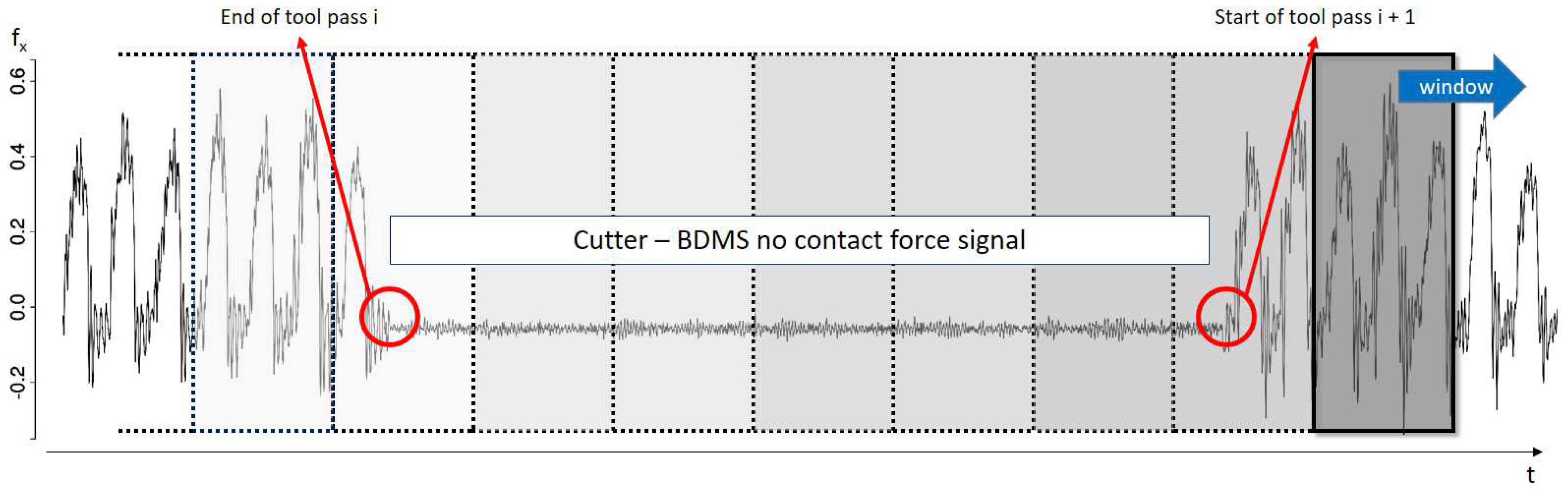
• Veracity: The sensory data were captured during the entire machining process. This includes force signals when the cutter is not touching the workpiece. Hence, the data contain different levels of trustworthiness, which had to be identified and treated at different application levels in order to ensure the correct harvesting and extraction of knowledge for gaining insight and learning.
• Variety: The sensory data, as well as the microscopic images define a plethora of data types categorised into structured data, i.e., information with a high degree of organisation, and unstructured data, i.e., information that has neither a pre-defined data model or organisation.

4.3. Data Cleansing

As described in Section 3.1, face milling is performed line-by-line with retraction and step over at the position feed rate along the x-axis. This implies that between the moment the cutter reaches the end of tool pass i and until it repositions to start tool pass $i+1$, the data generated by the dynamometer should be ignored as there is no contact between the cutter and the BDMS workpiece. In particular, these force values are very small when compared to the force values when cutting material. Hence, the Data Manager module has been enriched with a functionality that elegantly identifies and removes such no contact force values. In order to do this, a script that parses batches of technical data management streaming (TDMS) files has been configured with a fixed size window that moves from the beginning to the end of the collected force signals across the three axes. The windows move along a given signal with a null stride, i.e., no overlapping, searching for a subsequence of very small force values. Once such subsequence is sought, the beginning of it is marked, and the window continues moving until contiguous sufficiently large force values are identified, as shown in Figure 5. Thus, all small force values from the beginning until the end of the subsequence are removed.

5. Online Tool Wear Classification

The online tool wear classification system comprises a model building stage, a model training and testing stage and an online validation stage. The first one employs the condition monitoring infrastructure and the big data collection modules of the computing architecture with the aim to define and configure a CNN Model for classification. The second stage is in charge of fine tuning and assessing this model, which will be used to configure the Classifier module of the computing architecture. The last stage aims at demonstrating the seamless coordination of the monitoring infrastructure and the classification modules of the computing architecture in real time.

5.1. Model Building

Three tasks take place during this stage: force signals’ collection, wear calculation and the CNN Model creation. The first task concerns force values’ acquisition from milling experiments; the second one involves tool flank wear measurements; whereas the third one combines all these data to build, train and test a CNN Model systematically.

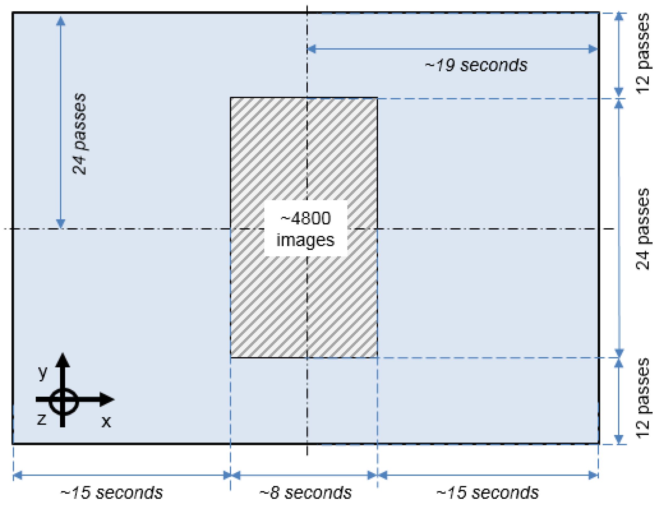
5.1.1. Signals Collection

In order to conduct force signal collection, the CNC machining centre was programmed with the cutting parameters described in Section 3.1 to perform nine layers of 48 tool passes each. In particular, this total number of passes was done in two blocks of 24 tool passes as a compromise between available time and the need to monitor the progress of the tool wear through a digital microscope; hence, removing two halves of material per layer referred to as $LayerAB\_CD$ where $AB$ is the layer number ranging from 01–09 and $CD$ is either 01 for the first half layer or 02 for the second half layer. Thus, the Signal Reader module was configured with $NIcDAQ9191$ (National Instruments NI-9191) as the device name, 50 kHz as the sampling rate and TDMS-formatted files as external storage named $LayerAB\_CD\_YYYY\_MM\_DD.TDMS$ (where $YYYY\_MM\_DD$ is the date of the file). Since each of these files contains force values sampled at 50 kHz and a tool pass lasts nearly 38 s, then the total number of triplets in one layer is $91.2$ million, which accounts for $820.8$ million triplets across the nine layers. The total time it took to conduct these experiments is equivalent to an operator’s shift, and the total number of TDMS files accounts for nearly 7 GB of data.

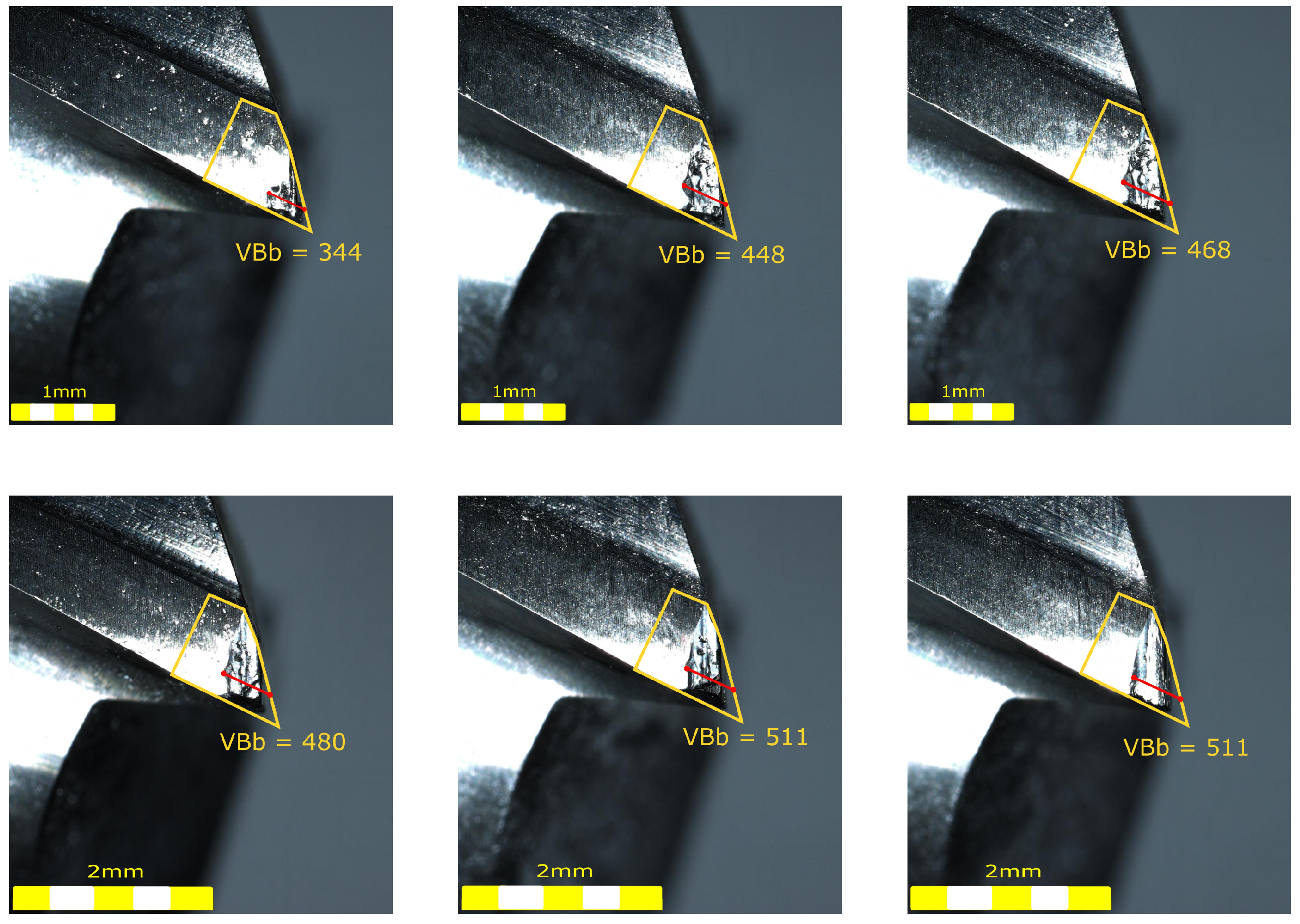
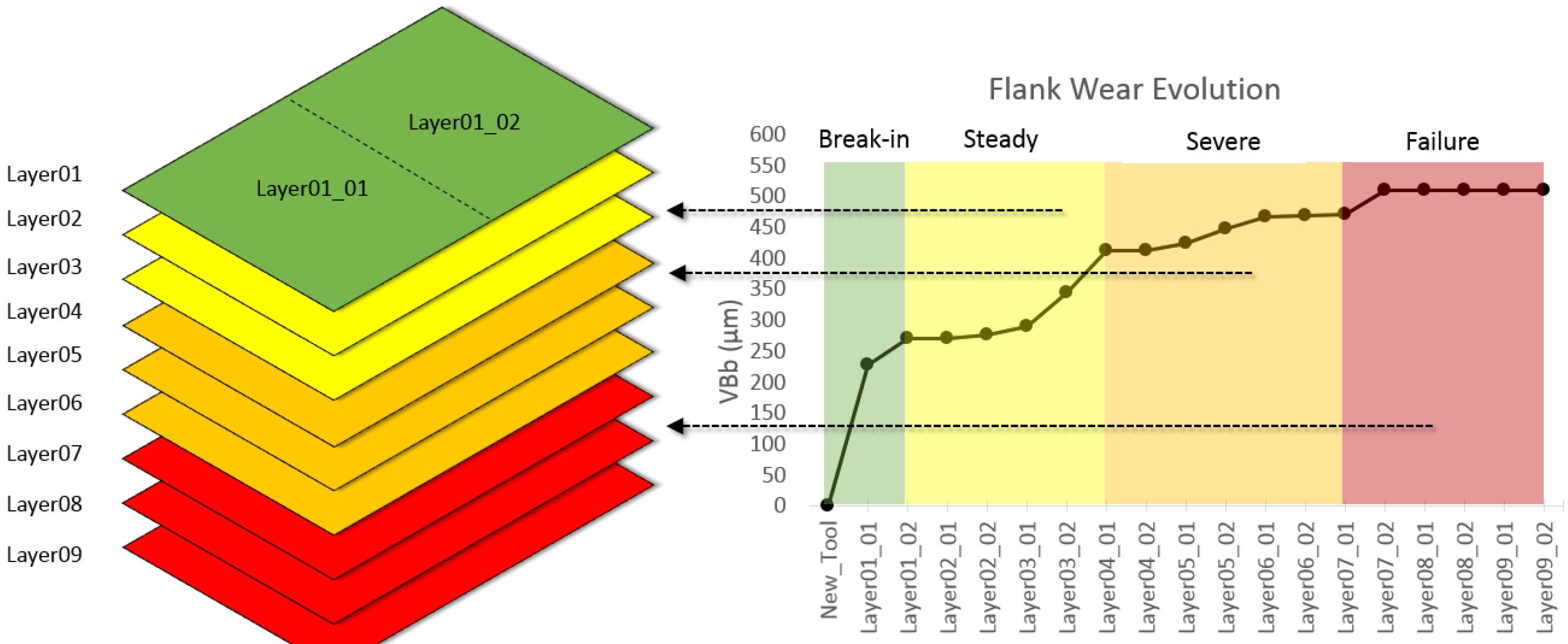
5.1.2. Tool Wear Calculation

In order to perform the wear calculation, the tool was subject to microscopic imaging every 24 tool passes. This was conducted on both flutes, referred to as Flute 1 and Flute 2, using the Olympus DSX110 digital industrial microscope. Each of the resulting flute images was compared to an image of the same flute when the tool was new. This comparison highlighted the differences between the geometries of the worn and new flute edges and enabled the determination of a value in micrometres ($\mathsf{\mu }\mathrm{m}$), which was representative of the actual wear. This procedure was consistently followed across this stage. Examples of images’ comparison and wear calculations are shown in Figure 6.

The eighteen flank wear values were employed to construct a plot that reflects the evolution of the tool flank wear across the nine layers, as shown at the right-hand side of Figure 7. As a result, four tool wear stages can be identified at this plot. These stages are identified based on the change of the curve’s gradient as the Break-in class for measurements below $280\mathsf{\mu }\mathrm{m}$, the Steady class for measurements ranging from 280–$410\mathsf{\mu }\mathrm{m}$, the Severe class for measurements ranging from 410–$480\mathsf{\mu }\mathrm{m}$ and the Failure class for those measurements above $480\mathsf{\mu }\mathrm{m}$.

5.1.3. Model Creation

In order to perform the CNN Model creation, a CNN model was instantiated from the Tensorflow library [45,46]. This has been configured with a six-level architecture comprised of two sets of convolution/ReLU and pooling layers (Levels 1–4) to perform feature detection, followed by a fully-connected multilayer perceptron (MLP) (Levels 5 and 6) to perform the classification. Since this architecture has been previously implemented and successfully tested for the classification of three-channel images (CIFAR-10 dataset [47]), it was decided to use it as an off-the-shelf starting point. The size of the kernels used was determined by the size of the images encoded by the GASF component. Given that this component is typically capturing three complete revolutions of the tool in one image (six cycles of the signal, as the tool has two flutes), the kernel of the first convolution was set to a size of 16, which allows one to “capture” a third of the signal cycle. The stride of the kernel was set to length four, due to the size of the image, allowing one to reduce the feature map (output) by a fourth. The pooling layer that follows uses a kernel of size three, which allows a further reduction of the feature map to a size of $32\times 32$. This is enough to keep the detected low-level features that will be grouped into higher level ones by the following convolution. The remaining layers use kernels of size eight and three, containing the high-level features in feature maps of size $16\times 16$. These are fed to the fully-connected MLP that is finally connected to four outputs, one for each tool wear class. A summary of the architectural components of the CNN Model together with their input parameter values are shown in

Table 1. Parameter values employed during the training of the CNN model.

CNN Level	Type	Input Size	Kernel Size	Stride	Output Size	Filters
1	Convolution	$256\times 256\times 3$	$16\times 16\times 3$	4	$64\times 64$	64
2	Pooling	$64\times 64\times 64$	$3\times 3$	3	$32\times 32$	64
3	Convolution	$32\times 32\times 64$	$8\times 8$	1	$32\times 32$	64
4	Pooling	$32\times 32\times 64$	$3\times 3$	2	$16\times 16$	64
5	Fully-connected	384				192
6	Fully-connected	192				4

.

5.2. Model Training and Testing

The eighteen TDMS files were employed for training and testing the CNN Model. In order to disregard any potential noise that could be affecting the force signals, only those values captured at a specific area of the workpiece were considered for training and testing (shaded area in Figure 8). This chosen area comprises the eight central seconds along the 24 central passes. Therefore, the total number of triplets considered for training and testing the CNN Model was reduced to $86.5$ million. During the training and testing stage of the CNN Model, arrays of triplets were systematically sampled from the nine central areas. The length of the arrays was defined to be 2000 consecutive triplets, which accounts for 43,200 unique arrays across the nine layers. Due to the computing power restrictions, this size was further reduced, which results in a sampling set of 1428 arrays of triplets partitioned into $70\%$ as the training set (i.e., 1000 sequences) and $30\%$ as the testing set (i.e., 428 sequences).

5.2.1. Model Training

The training stage should carefully consider the correspondence between the tool wear classes and the layers. It is important to note that if the number of layers associated with the four tool wear classes was uniformly distributed, then an equivalent number of arrays could be sampled from each layer. However, as shown in Figure 7, each tool wear class has a different quantity of associated layers; hence, a class imbalance problem may arise. Therefore, an equal sampling percentage (i.e., 25% of the training set) was associated per class, which in fact required, for some classes, to sample across different numbers of layers. For instance, for the Break-in class, it is required to sample from only one layer, whereas for the Failure class, it is required to sample from three different layers. Thus, after systematically sampling arrays of triplets from the training set, these are used as input to the GASF component [39], which performs two main tasks. First, it generates an image of $256\times 256$ pixels for each of the force components of the sequence; second, it compiles and creates a three-channel object with the created images. Once the complete training set is encoded as three-channel objects, these are loaded to the CNN Model in batches of 100 without repetition and presented to the network until the complete training set has been seen once. The loss is then calculated and the weights modified. This comprises one iteration of the training process, which is repeated 1000 times.

5.2.2. Model Testing

During the testing stage, all arrays of triplets from the testing set are selected in turns and fed into the CNN Model. Thus, the performance of the CNN Model was assessed in terms of a confusion matrix (see

Table 2. The confusion matrix with the results obtained with the test set.

Predicted/Actual	Break-In	Steady	Severe	Failure	Total
Break-in	102	5	5		112
Steady	4	88	10	5	107
Severe	1	8	71	28	108
Failure		6	21	74	101
Total	107	107	107	107

) and by calculating the accuracy or success rate. The confusion matrix categorizes predictions of the classes according to whether they match the actual classes. The success rate is calculated in terms of the number of true positives, false positives, true negatives and true positives. In particular, the CNN model employed here has achieved an overall accuracy of $78\%$. Looking at classes individually, the accuracy obtained for the Break-in class is $95\%$, the highest among all classes. The accuracy obtained for the Steady, Severe and Failure classes is $82.2\%$, $66.3\%$ and $69\%$, respectively. These results show that testing sequences from layers associated with the Severe and Failure classes are more difficult to classify. From the cases incorrectly classified for the Severe class, a smaller percentage is under-classified, compared to the ones classified as Failure. Although this percentage is low, it is important to look further into these cases to understand the cause. From a visual inspection of the data, it is evident that the force signals become more heterogeneous as the tool starts wearing out, which could explain the variability of the results in the Severe and Failure classes. Nevertheless, the results obtained are promising as the classification can be performed from a consensus of several classification samples rather than on a single sample.

5.3. Online Validation

The aim of this type of validation is to report the progression of the tool flank wear online, that is during dry machining. On the one hand, the monitoring infrastructure was set up with the same machining conditions as before, that is a new two-flute $6\mathrm{mm}$ solid carbide end milling cutter, a new $180\times 125\times 25{\mathrm{mm}}^3$ BDMS workpiece, compressed air for dry machining and cutting parameters fixed to $S=4775\mathrm{RPM}$, $f=287\mathrm{mm}/\min$, $a_e=2.7\mathrm{mm}$ and $a_p=0.3\mathrm{mm}$. Thus, since the face milling was performed in the same fashion as described in Section 3.1, the removal of one layer of material in the BDMS block accounts for a total of 48 tool passes. On the other hand, the computing architecture was set up with the Classifier module using the CNN Model built in Section 5.1 and the Signal Reader module configured with 50 kHz as the sampling rate and, in particular, to perform readings of 1 s in length for each of the 48 tool passes inside the shaded area depicted in Figure 9. Each of these readings accounts for a sequence of 50,000 triplets, which were used to randomly choose ten non-repetitive arrays of 2000 consecutive triplets each. These were then passed, in turns, to the GASF component to convert them into images and feed the CNN Model. At this point in time, classification took place with the model expected to report the best class that reflects the current stage of the tool wear.

The progress of the classification, a sample of the forces, as well as the result of the current classification were constantly displayed by the GUI module. For instance, six representative examples of the online tool wear classification during validation are shown in Figure 10, where classes are coloured coded in green for Break-in, yellow for Steady, orange for Severe and red for Failure, and values along the x-axis of the plot denote the number of passes for the current layer.

On the one hand, it is clear that there is a smooth transition between the Break-in class to the Steady class within the first two layers, a transition between the Steady class and the Severe class between third and fifth layer and a transition between the Severe and the Failure class from the fifth layer onwards. On the other hand, it is also possible to observe that some force signals have been wrongly classified by the CNN Model. Examples of these are the two Failure classes reported in the first layer or the Break-in class reported in the eighth layer, as marked by red circles in Figure 10. After some investigations, this misclassification seemed to be related to a lack of synchronization between components of the computing architecture and the monitoring infrastructure, for example the signal was acquired when the tool was cutting just before the end of the workpiece. As one of the initial results, however, it could overall be concluded that the CNN Model has managed to classify the force signals successfully, collected in real time, of a new milling process. In fact, it is important to consider that the force signals were originated by a physically-controlled process where hardness was not uniformly distributed across the workpiece material and end mill carbide tools were never equal, but similar. All these give room to a certain degree of uncertainty, which converts milling into a stochastic process, hence making the results of the validation vary within a certain range when repeated.

6. Conclusions and Further Work

This paper presented an indirect online condition monitoring system that exploits a vast amount of high frequency generated sensory data with deep learning. In particular, it reported on:

• An online tool wear classification system built in terms of a monitoring infrastructure, dedicated to performing dry milling on steel while capturing force signals in real time, and a computing architecture, assembled for the real-time assessment of the flank wear based on deep learning.
• An approach based on a very simple mathematical model that converts raw force signals into two-dimensional images (the GASF component) that, when used as input to an off-the-shelf CNN architecture, exploits internal spatial structures encoding edge devastation for reporting tool wear progression during dry machining on steel.
• An end-to-end smart system that exploits big data for the development of online indirect tool condition monitoring that is free of feature engineering, a signal analyst or image processing expertise. An offline test has successfully reported an accuracy of $78\%$ followed by an online validation that classifies force signals acquired in real time from a new milling process.

Overall, this approach has demonstrated that a big data analytics method for classification applied to large volumes of continuously-acquired force signals generated at high speed during dry milling responds sufficiently well when used as an indicator of the different stages of tool wear.

Given the successful results, further work from different perspectives is left to be explored. From the methodological perspective, additional experiments will be carried out employing tools of different diameters and under different cutting conditions. The data generated from these experiments will be used to develop a new deep learning model with the aim to transition towards a more general, robust and resilient monitoring system that can be used for tracking the wear progression on different types of cutters. From the technical perspective, an extension of this smart methodology could include signals from other sensor (individually and combined) such as acoustic emission and acceleration. This could enhance the presented approach with a more accurate picture of the progression of the wear since information from different dimensions might uncover specific characteristics that remain hidden when only using force signals. In order to do this, either the current CNN model could be enriched with additional inputs and a higher order architecture, or separate ensembles of similar CNN models could work in an integrated fashion. In addition, the updated tool monitoring approach described in this paper could be used to inform an adaptive control scheme, the synergy of which would maximise the remaining useful life of a tool; thus, bringing the completion of an end-to-end online condition monitoring system much closer to automation. From the application domain perspective, since the tool wear classification system uses cutting force measurements, the overall approach presented here could also be applied to other machining processes with minimal changes on the condition monitoring infrastructure. For instance, a different type of force sensor may be required depending on the specific process. Once the force signals can be collected, the same software architecture can still be used to process data, classify and report the tool wear progress to the end user.

References

1. Federal Ministry of Education and Research. Project of the Future: Industry 4.0. 2017. Available online: https://industrie40.vdma.org/en/ueber-uns (accessed on 30 August 2018).
2. Lasi, H.; Fettke, P.; Feld, T.; Hoffmann, M. Industry 4.0. Bus. Inf. Syst. Eng. 2014, 6, 239–242. [Google Scholar] [CrossRef]
3. Zhong, Y.R.; Xu, X.; Klotz, E.; Newman, S.T. Intelligent Manufacturing in the Context of Industry 4.0: A Review. Engineering 2017, 3, 616–630. [Google Scholar] [CrossRef]
4. Kusiak, A. Smart manufacturing must embrace big data. Nature 2017, 544, 23–25. [Google Scholar] [CrossRef] [PubMed] [Green Version]
5. Tao, F.; Qi, Q.; Liu, A.; Kisiak, A. Data-driven smart manufacturing. J. Manuf. Syst. 2018, 48, 157–169. [Google Scholar] [CrossRef]
6. Sharp, M.; Ak, T.; Hedberg, T. A survey of the advancing use and development of machine learning in smart manufacturing. J. Manuf. Syst. 2018, 48, 170–179. [Google Scholar] [CrossRef]
7. Tsai, C.-W.; Lai, C.-F.; Chao, H.-C.; Vasilakos, A.V. Big data analytics: A survey. J. Big Data 2015, 2, 21–53. [Google Scholar] [CrossRef]
8. Kalpakjian, S.; Schmid, S. Manufacturing Engineering & Technology; Pearson: London, UK, 2014; ISBN-13 9780133128758. [Google Scholar]
9. Siddhpura, A.; Paurobally, R. A review of flank wear prediction methods for tool condition monitoring in a turning process. Int. J. Adv. Manuf. Technol. 2013, 65, 371–393. [Google Scholar] [CrossRef]
10. Zhou, Y.; Xue, W. Review of tool condition monitoring methods in milling processes. Int. J. Adv. Manuf. Technol. 2018, 96, 2509–2523. [Google Scholar] [CrossRef]
11. García-Ordás, M.T.; Alegre, E.; Gonzáles-Castro, V.; Alaiz-Rodríguez, R. A computer vision approach to analyze and classify tool wear level in milling processes using shape descriptors and machine learning techniques. Int. J. Adv. Manuf. Technol. 2017, 90, 1947–1961. [Google Scholar] [CrossRef]
12. Navarro, M.D.; Meseguer, M.D.; Sánchez, A.I.; Gutiérrez, S.C. Tool wear study in edge trimming on basalt fibre reinforced plastics. Procedia Manuf. 2017, 13, 259–266. [Google Scholar] [CrossRef]
13. Prado, M.T.; Pereira, A.; Pérez, J.A.; Mathia, T.G. Methodology for tool wear analysis by electrical measuring during milling of AISI H13 and its impact on surface morphology. Procedia Manuf. 2017, 13, 356–363. [Google Scholar] [CrossRef]
14. Sanchez, Y.; Trujillo, F.J.; Sevilla, L.; Marcos, M. Indirect Monitoring Method of Tool Wear using the Analysis of Cutting Force during Dry Machining of Ti Alloys. Procedia Manuf. 2017, 13, 623–630. [Google Scholar] [CrossRef]
15. Krishnakumar, P.; Rameshkumar, K.; Ramachandran, K.I. Tool Wear Condition Prediction Using Vibration Signals in High Speed Machining (HSM) of Titanium (Ti-6Al-4V) Alloy. Procedia Comput. Sci. 2015, 50, 270–275. [Google Scholar] [CrossRef]
16. Krishnakumar, P.; Rameshkumar, K.; Ramachandran, K.I. Feature level fusion of vibration and acoustic emission signals in tool condition monitoring using machine learning classifiers. Int. J. Progn. Health Manag. 2018, 9, 1–15. [Google Scholar]
17. Kong, D.; Chen, Y.; Li, N. Force-based tool wear estimation for milling process using Gaussian mixture hidden Markov models. Int. J. Adv. Manuf. Technol. 2017, 92, 2853–2865. [Google Scholar] [CrossRef]
18. Luo, B.; Wang, H.; Liu, H.; Li, B.; Peng, F. Early Fault Detection of Machine Tools Based on Deep Learning and Dynamic Identification. IEEE Trans. Ind. Electron. 2018, 66, 509–518. [Google Scholar] [CrossRef]
19. Jia, F.; Lei, Y.; Guo, L.; Lin, J.; Xing, S. A neural network constructed by deep learning technique and its application to intelligent fault diagnosis of machines. Neurocomputing 2018, 272, 619–628. [Google Scholar] [CrossRef]
20. Deng, L. A tutorial survey of architectures, algorithms, and applications for deep learning. APSIPA Trans. Signal Inf. Process. 2014, 3. [Google Scholar] [CrossRef] [Green Version]
21. LeCun, Y.; Bengio, Y.; Hinton, G. Deep learning. Nature 2015, 521, 436–444. [Google Scholar] [CrossRef] [PubMed]
22. LeCun, Y.; Bottou, L.; Bengio, Y.; Haffner, P. Gradient-based learning applied to document recognition. Proc. IEEE 1998, 86, 2278–2324. [Google Scholar] [CrossRef] [Green Version]
23. Jing, L.; Zhao, M.; Li, P.; Xu, X. A convolutional neural network based feature learning and fault diagnosis method for the condition monitoring of gearbox. Measurement 2017, 111, 1–10. [Google Scholar] [CrossRef]
24. Janssens, O.; Slavkovikj, V.; Vervisch, B.; Stockman, K.; Loccufier, M.; Verstockt, S.; Van de Walle, R.; Van Hoecke, S. Convolutional Neural Network Based Fault Detection for Rotating Machinery. J. Sound Vib. 2016, 377, 331–345. [Google Scholar] [CrossRef]
25. Zhao, R.; Yan, R.; Chen, Z.; Mao, K.; Wang, P.; Gao, R.X. Deep learning and its applications to machine health monitoring. Mech. Syst. Signal Process. 2019, 115, 213–237. [Google Scholar] [CrossRef]
26. Weimer, D.; Scholz-Reiter, B.; Shpitalni, M. Design of deep convolutional neural network architectures for automated feature extraction in industrial inspection. CIRP Ann. 2016, 65, 417–420. [Google Scholar] [CrossRef]
27. Wang, P.; Ananya; Yan, R.; Gao, X.R. Virtualization and deep recognition for system fault classification. J. Manuf. Syst. 2017, 44, 310–316. [Google Scholar] [CrossRef]
28. Shevchik, S.A.; Kenel, C.; Leinenbach, C.; Wasmer, K. Acoustic emission for in situ quality monitoring in additive manufacturing using spectral convolutional neural networks. Addit. Manuf. 2018, 21, 598–604. [Google Scholar] [CrossRef]
29. Aghazadeh, F.; Tahan, A.; Thomas, M. Tool condition monitoring using spectral subtraction and convolutional neural networks in milling process. Int. J. Adv. Manuf. Technol. 2018, 98, 3217–3227. [Google Scholar] [CrossRef]
30. Kothuru, A.; Nooka, S.; Liu, R. Audio-Based Tool Condition Monitoring in Milling of the Workpiece Material With the Hardness Variation Using Support Vector Machines and Convolutional Neural Networks. J. Manuf. Sci. Eng. 2018, 140, 111006. [Google Scholar] [CrossRef]
31. Shi, C.; Panoutsos, G.; Luo, B.; Hongqi, L.; Li, B.; Lin, X. Using multiple feature spaces-based deep learning for tool condition monitoring in ultra-precision manufacturing. IEEE Trans. Ind. Electron. 2018. [Google Scholar] [CrossRef]
32. Khan, S.; Yairi, T. A review on the application of deep learning in system health management. Mech. Syst. Signal Process. 2018, 107, 241–265. [Google Scholar] [CrossRef]
33. Li, S.; Liu, G.; Tang, X.; Lu, J.; Hu, J. An Ensemble Deep Convolutional Neural Network Model with Improved D-S Evidence Fusion for Bearing Fault Diagnosis. Sensors 2018, 17, 1729. [Google Scholar] [CrossRef] [PubMed]
34. Chen, Y.; Jin, Y.; Jiri, G. Predicting tool wear with multi-sensor data using deep belief networks. Int. J. Adv. Manuf. Technol. 2018. [Google Scholar] [CrossRef]
35. Wu, J.; Su, Y.; Cheng, Y.; Shao, X.; Deng, C.; Liu, C. Multi-sensor information fusion for remaining useful life prediction of machining tools by adaptive network based fuzzy inference system. Appl. Soft Comput. 2018, 68, 13–23. [Google Scholar] [CrossRef]
36. Madhusudana, C.K.; Kumar, H.; Narendranath, S. Face milling tool condition monitoring using sound signal. Int. J. Syst. Assur. Eng. Manag. 2017, 8, 1643–1653. [Google Scholar] [CrossRef]
37. Kilundu, B.; Dehombreux, P.; Chiementin, X. Tool wear monitoring by machine learning techniques and singular spectrum analysis. Mech. Syst. Signal Process. 2011, 25, 400–415. [Google Scholar] [CrossRef]
38. Fu, Y.; Zhang, Y.; Qiao, H.; Li, D.; Zhou, H.; Leopold, J. Analysis of Feature Extracting Ability for Cutting State Monitoring Using Deep Belief Networks. Procedia CIRP 2015, 31, 29–34. [Google Scholar] [CrossRef]
39. Gouarir, A.; Martínez-Arellano, G.; Terrazas, G.; Benardos, P.; Ratchev, S. In-Process Tool Wear Prediction System Based on Machine Learning Techniques and Force Analysis. Procedia CIRP 2018, 77, 501–504. [Google Scholar] [CrossRef]
40. Nyquist, H. Certain topics in telegraph transmission theory. IEE Trans. 1928, 47, 617–644. [Google Scholar] [CrossRef]
41. Complete Guide to Building a Measurement System. National Instruments. Available online: http://www.ni.com/gate/gb/GB_EKITDAQSYS/US (accessed on 14 August 2018).
42. Kistler Multicomponent Dynamometer. Kistler Group. Available online: https://www.kistler.com/en/product/type-9255c/ (accessed on 14 August 2018).
43. Ferry, N.; Terrazas, G.; Kalweit, P.; Solberg, A.; Ratchev, S.; Weinelt, D. Towards a Big Data Platform for Managing Machine Generated Data in the Cloud. IEEE Int. Conf. Ind. Inform. 2017, 263–270. [Google Scholar] [CrossRef]
44. Babiceanu, R.F.; Seker, R. Big Data and virtualization for manufacturing cyber-physical systems: A survey of the current status and future outlook. Comput. Ind. 2016, 81, 128–137. [Google Scholar] [CrossRef]
45. Abadi, M.; Agarwal, A.; Barham, P.; Brevdo, E.; Chen, Z.; Citro, C.; Corrado, G.S.; Davis, A.; Dean, J.; Devin, M.; et al. Tensorflow: Large-scale machine learning on heterogeneous distributed systems. arXiv, 2016; arXiv:1603.04467. [Google Scholar]
46. Tensorflow, Convolutional Neural Networks. Available online: https://www.tensorflow.org/tutorials/deep_cnn (accessed on 23 January 2018).
47. Krizhevsky, A. Learning Multiple Layers of Features From Tiny Images. Available online: http://www.cs.toronto.edu/~kriz/cifar.html (accessed on 23 January 2018).
Figure 1. The condition monitoring comprising a dynamometer that measures force and outputs voltage signals (in pC) to a charge amplifier. The amplified voltage (in mV) is a signal sent to analogue-to-digital converter (ADC) modules, the outputs of which are stored and accessed via computer bus devices.
Jmmp 02 00072 g001
Figure 2. (a) The Hermle C20U CNC machine together with its Heidenhain iTNC 530 control. (b) Interior of the CNC machine equipped with a tool (1), compressed air nozzles (2), a workpiece (3) and a three-component force sensor dynamometer Kistler 9255B(4).
Jmmp 02 00072 g002
Figure 3. The computing architecture for real-time tool wear classification. The big data collection comprises the Signal Reader and the Data Manager modules to sample force values and externally store them. The tool wear classification comprises the Signal Reader, the Classifier and the GUI modules that selectively sample force values and classify them.
Jmmp 02 00072 g003
Figure 4. The tool wear monitoring dashboard displayed by the GUI module. The top part displays the real-time forces on the three axes, and the bottom part contains machining parameters and associated information, a gauge with the actual tool wear level and a history of the tool wear progression.
Jmmp 02 00072 g004
Figure 5. Detection for the removal of the no contact force signal between the cutter and the bright drawn mild steel (BDMS) workpiece. A fixed size window moves along the acquired signal searching for the start and end of a small subsequence of very small values denoting the end of tool pass i and start of tool pass i + 1 .
Jmmp 02 00072 g005
Figure 6. From left to right and top to bottom, flank wear measurement VBb (in μ m ) conducted on: Flute 1 after milling L a y e r 03 _ 02 , L a y e r 05 _ 02 , L a y e r 06 _ 01 , L a y e r 07 _ 02 , L a y e r 08 _ 01 and L a y e r 09 _ 01 .
Jmmp 02 00072 g006
Figure 7. Mapping between the evolution of the tool flank wear across the Break-in, Steady, Severe and Failure classes (right-hand side) to the nine layers (left-hand side).
Jmmp 02 00072 g007
Figure 8. Schematic representation of a workpiece layer with the approximate duration of a tool pass (in seconds) and the total number of tool passes per layer. The shade depicts the area where the force values are chosen for training.
Jmmp 02 00072 g008
Figure 9. Schematic representation of a workpiece layer with the approximate duration of a tool pass (in seconds) and the total number of tool passes per layer. The shade depicts the area where the force values are chosen for validating of the CNN model in real time.
Jmmp 02 00072 g009
Figure 10. Representative examples of the online tool wear classification. Classes are colour coded as green for Break-in, yellow for Steady, orange for Severe and red for Failure, whereas values along the x-axis denote the number of passes for the current layer.
Jmmp 02 00072 g010