Article

Numerical Study on the Temperature-Dependent Viscosity Effect on the Strand Shape in Extrusion-Based Additive Manufacturing

1
Department of Chemical and Biomolecular Engineering, Vanderbilt University, Nashville, TN 37235, USA
2
Department of Chemical and Biochemical Engineering, Missouri University of Science and Technology, Rolla, MO 65409, USA
3
Department of Mechanical and Aerospace Engineering, Missouri University of Science and Technology, Rolla, MO 65409, USA
4
Department of Biomedical, Biological and Chemical Engineering, University of Missouri, Columbia, MO 65211, USA
*
Author to whom correspondence should be addressed.
J. Manuf. Mater. Process. 2020, 4(2), 46; https://doi.org/10.3390/jmmp4020046
Submission received: 8 April 2020 / Revised: 5 May 2020 / Accepted: 13 May 2020 / Published: 15 May 2020
(This article belongs to the Special Issue Additive Manufacturing and Device Applications)

Abstract

:
A numerical model that incorporates temperature-dependent non-Newtonian viscosity was developed to simulate the extrusion process in extrusion-based additive manufacturing. Agreement with the experimental data was achieved by simulating a polylactic acid melt flow as a non-isothermal power law fluid using experimentally fitted parameters for polylactic acid. The model was used to investigate the temperature effect on the flow behavior, the cross-sectional area, and the uniformity of the extruded strand. OpenFOAM, an open source simulation tool based on the finite volume method, was used to perform the simulations. A computational module for solving the equations of non-isothermal multiphase flows was also developed to simulate the extrusion process under a small gap condition where the gap between the nozzle and the substrate surface is smaller than the nozzle diameter. Comparison of the strand shapes obtained from our model with isothermal Newtonian simulation, and experimental data confirms that our model improves the agreement with the experimental data. The result shows that the cross-sectional area of the extruded strand is sensitive to the temperature-dependent viscosity, especially in the small gap condition which has recently increased in popularity. Our numerical investigation was able to show nozzle temperature effects on the strand shape and surface topography which previously had been investigated and observed empirically only.

1. Introduction

Extrusion-based additive manufacturing, also called fused deposition modeling (FDM) or fused filament fabrication (FFF), is a type of additive manufacturing (AM) process which fabricates a 3D part by building up extruded material layer by layer. A common choice of raw material for FDM is thermoplastic polymers such as polylactic acid which is used in this study. A typical FDM process consists of the following steps: (1) A thermoplastic filament is fed into the printer head, which consists of a liquefier and a nozzle. (2) The filament is heated in the liquefier to just above its melting temperature to reach a semi-molten state. (3) The molten filament is extruded through the nozzle. (4) The extruded polymer is deposited on a substrate or on a previously extruded strand. (5) The deposited strand cools down to become a solid layer. If that strand is deposited adjacent to another strand, those strands fuse together.
Due to the ability of FDM to rapidly and efficiently fabricate a complicated structure with the help of computer-aided automation, there have been many applications and developments in the field [1,2,3]. However, parts manufactured using FDM have problems with low mechanical strength, high surface roughness, delamination, and major anisotropy. Studies have related process parameters, such as operation temperature and feed velocity, to the final mechanical and thermal properties for better prediction and control of the final part properties. Empirical modeling relating the process parameters and the final properties was one of those approaches [4]. Computational fluid dynamics (CFD) simulation, on the other hand, has been used for a deterministic approach [5,6,7,8]. Since accurate prediction of extruded strand shape is required for controlling the mechanical and structural properties of a final part [8,9,10], the CFD approach has garnered attention.
One such CFD simulation study of an extrusion-based additive manufacturing process was done by Bellini [5]. Extrusion through a nozzle and the subsequent deposition of a ceramic melt flow was simulated assuming shear-thinning (or power-law) and temperature-dependent behaviors. Although the material flow was not a polymer melt, the viscosity model is generally applicable to simulations of polymer flows. Many of these simulations have focused on the dynamics inside the liquefier. For example, Ramanath et al. [11] simulated a flow of poly-ε-caprolactone in a nozzle for an FDM process. They focused on studying the effects of nozzle geometry and filament inlet velocity on the flow behavior, temperature distribution, and pressure drop where the polymer flow was assumed to be an isothermal shear-thinning fluid. A similar method was applied in the simulation of the flow of an acrylonitrile-butadiene-styrene/iron composite in a liquefier [12].
In contrast to the liquefier simulations, simulations of the extrusion and deposition of polymer flows are more difficult due to the free surface and the very high viscosity. For simplicity, some simulations have used an isothermal Newtonian fluid model [13,14,15]. These authors claimed that the isothermal Newtonian assumption was accurate enough in comparison to experimental data. A subsequent study directly compared the strand cross-sectional areas from experimental data to the simulation results and showed that an isothermal Newtonian simulation can match the relation with the strand shape and the process conditions from the experiment [15]. However, this agreement was only for the case where the gap between the nozzle and the substrate is similar to the nozzle diameter, and discrepancies were reported for the case of a smaller gap. Although the study claimed that the small gap condition is not typical for FDM, a smaller gap has been utilized in recent developments [16,17].
In this study, we performed CFD simulations to investigate the effect of the temperature-dependent viscosity on the strand shape, particularly cross-sectional area, in the small gap extrusion condition. Since the viscosity is sensitive to temperature, we hypothesize that temperature-dependent viscosity affects the flow behaviors in the deposition flow and, consequently, the strand shape. There have been studies describing the temperature effect on strand deformation; but many of these studies only focused on the solid state [18,19], and the extrusion process was not considered [20]. Other simulation studies have focused on both viscoelasticity and temperature-dependent viscosity [21,22,23]. McIlroy and Olmsted focused on the polymer molecular structure in the deposition flow right after extrusion [21]. Liu et al. only performed a 2D simulation. They did consider temperature-dependent solidification, but the viscosity in the liquid phase remained constant [22]. Xia et al. showed that viscoelasticity affects the strand shape, however, their maximum viscosity was set to 5000 Pa∙s, which seemed to result in the simulated strands looking more liquid-like than the actual experimental behavior [23]. In this study, we use the rheological data of a polylactic acid (PLA) filament, which is commonly used in FDM as well as in many biomedical applications [24,25], and compare the simulated polymer behavior with the strand shape experimentally measured by Serdeczny et al. [15].
This paper is organized as follows: Section 2 describes our simulation method along with the model parameters for shear-thinning and temperature-dependent viscosity. In Section 3.1, a time-evolution of an extruded strand simulated by our model is shown. In Section 3.2, the strand shapes extruded from different process conditions obtained from our simulations are compared with the experimental observations and the isothermal Newtonian simulation results. In Section 3.3 and Section 3.4, the effects of the nozzle temperature on the strand shape and the surface roughness are investigated. Section 4 summarizes the findings and describes the future works.

2. Numerical Simulation

2.1. Governing Equations

The extrusion and deposition of a polymer melt flow is simulated as a free surface flow with temperature and shear rate dependent viscosity. The following governing equations can describe the flow behaviors in both liquid and gas phases:
ρ t + · ( ρ u ) = 0
( ρ u ) t + · ( ρ uu ) = p · τ + ρ g
where ρ, u, p and g are density, fluid velocity vector, pressure, and gravitational acceleration, respectively. The gas phase is assumed as air and the liquid phase as a PLA melt. More specifically, we chose the properties of a PLA filament used in the work by Phan et al. [24] (see the next section). The stress tensor, τ, is described by a power-law model:
τ = K ( Δ : Δ 2 ) n 1 2 Δ
where K and n are power-law model consistency and index, respectively. The velocity gradient tensor is defined as Δ ≡ ∇u + ∇uT. We used the Arrhenius relation for the consistency of a shear thinning fluid, K, to describe the temperature effect on the polymer viscosity according to a study on PLA rheology [24]:
K = K 0 exp ( f ( 1 / T 1 / T 0 ) )
where T is temperature in Kelvin and K0 is the value of K at a reference temperature, T0. The variation of K with T is governed by the parameter, f, which is obtained by fitting experimental data.
The temperature distribution in the PLA flow is solved by the energy equation:
( ρ c P T ) t + · ( u ρ c P T ) = k 2 T
where cp and k are specific heat capacity and thermal conductivity, respectively. We assume that there is no heat generation or viscous dissipation since it was found that its contribution to a 1-K temperature rise is less than 5% (personal communication with Dr. M. Mackay, the author of Ref [24,26]).
Our simulation uses the volume of fluid (VOF) approach to simulate the two-phase system. In VOF, as an Eulerian approach, a color function at each position x and time t is defined as:
ϕ ( x , t ) = { 1   for   x D l   at   time   t 0   for   x D g   at   time   t
where Dl and Dg are domains of liquid and gas, respectively [27]. If the color function is averaged over the volume of a cell, Vcell, the liquid fraction of the cell is calculated as:
α ( x i , t ) = 1 V c e l l V c e l l ϕ ( x , t ) dV
where xi is the i-th cell in the domain. The density at each position and time, then, is:
ρ ( x , t ) = ρ l ϕ ( x , t ) + ρ g ( 1 ϕ ( x , t ) )
By replacing the density in the continuity Equation (1) with the density defined in Equation (8), another governing equation for the liquid fraction of the cell is derived:
α t + · ( α u ) = 0

2.2. Numerical Model Solver

We performed the CFD simulation utilizing OpenFOAM, an open source CFD software based on a finite volume method. Various modules, based on object-oriented programming, for solving different equations for various CFD problems are available online. For velocity-pressure coupling (solving Equations (1) and (2)), the PIMPLE algorithm was adapted. The PIMPLE algorithm is a combination of PISO (Pressure Implicit with Splitting of Operators) and SIMPLE (Semi-Implicit Method for Pressure-Linked Equations). The PISO algorithm works well in solving transient problems while the SIMPLE algorithm works for steady-state problems. Thus, the PIMPLE algorithm can solve steady-state problems as well as transient problems and can do so using larger time-steps than the PISO algorithm. Further information regarding the PIMPLE algorithm can be found in [28].
In OpenFOAM, users can modify existing modules or develop their own modules for their own problems. In our study, we developed a new solver for non-isothermal free surface flows by improving an existing solver called “InterFoam” which is used for isothermal, incompressible, immiscible, two-phase fluids based on VOF. The new solver accounts for the non-isothermal nature of the extrusion process by including the Arrhenius model for the power law model consistency (Equation (4)) and the energy equation (Equation (5)). It is aimed to simulate transient free surface problems where transport properties vary with temperature. To accomplish this, the energy equation was coupled with the continuity (Equation (1)) and the momentum equations (Equation (2)). Similar to “InterFoam”, both phases are considered incompressible. It was assumed that the dependence of liquid viscosity on temperature follows Equation (4). The validation of our new solver is shown in Appendix A.

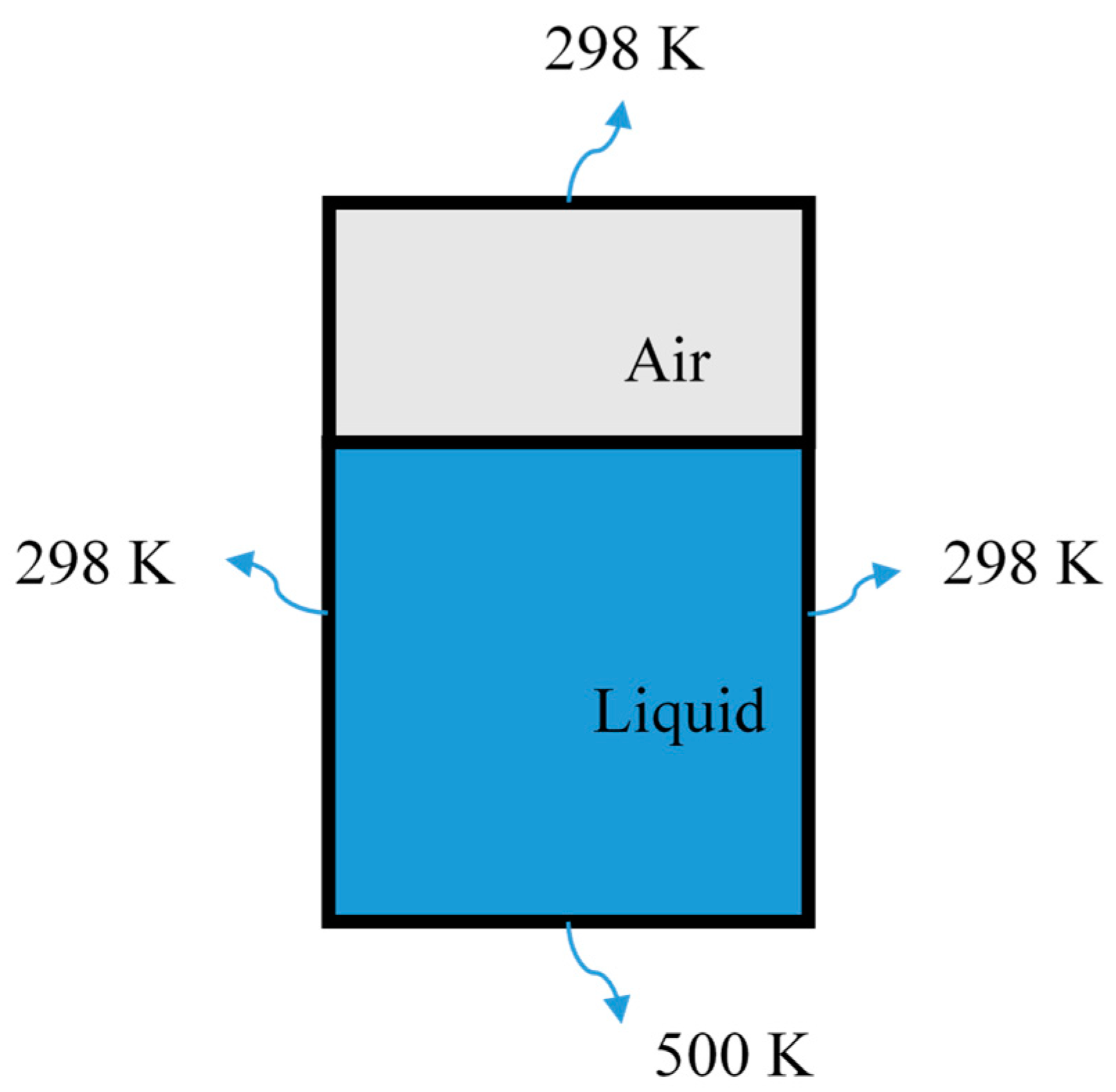
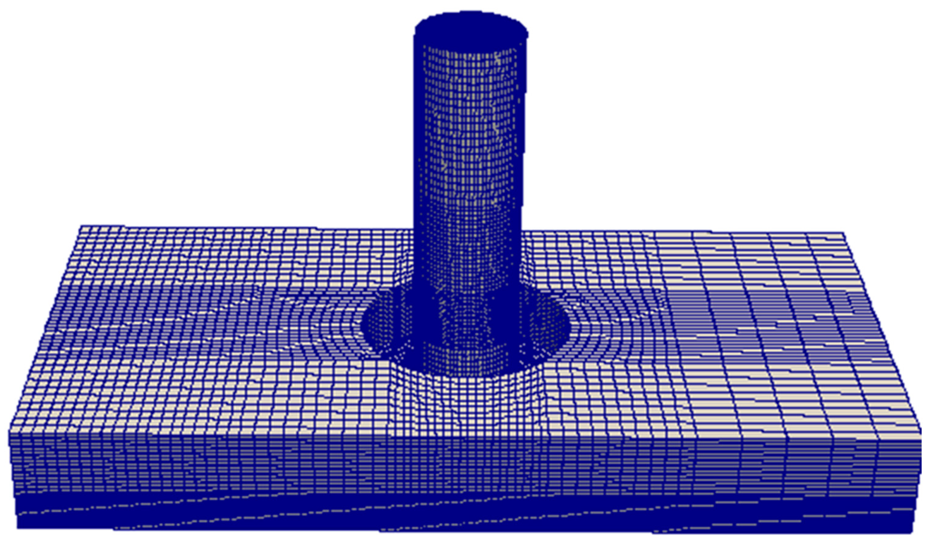
2.3. System Description

Figure 1 depicts the simulated system which consists of a cylindrical nozzle, a substrate plate, and the surrounding atmosphere. The nozzle has an inner diameter of d = 0.4mm and outer diameter of 2d. We chose the cylindrical nozzle for the purpose of comparing with the published experimental data by Serdeczny et al. [15].The gap distance between the nozzle exit and the substrate plate is g; we are particularly interested in the small gap condition g/d = 0.4, which is a condition where the isothermal Newtonian simulation showed a considerable discrepancy from the experimental data [15]. A viscous polymer melt inside the nozzle with an average flow velocity (the z-component of u is averaged over a cross-section of the nozzle) of <u> = 0.02 m/s is extruded through the nozzle. In this simulation, instead of moving the nozzle horizontally, the nozzle is stationary while the substrate plate moves horizontally at three different velocities, (U = 0.02, 0.015 and 0.01 m/s). The no-slip boundary condition is imposed on the nozzle wall as well as the substrate surface. The liquid-air interface has the boundary condition of equal stress and velocity on each phase. The air velocity at the top of the surrounding atmosphere domain is set to 0. The distance between the top of the surrounding atmosphere and the substrate plate was chosen as 0.76 mm, which does not affect the result of the simulated strand shape while maintaining a reasonable computational load. As shown in Figure 2, a hexahedral grid was used for meshing the 3D simulation domain which resulted in 242,000 cells. Velocity profiles simulated in finer meshes did not give noticeable differences.
Temperatures inside the nozzle and in the surrounding air were initially set to 463–503 and 298 K, respectively. Nozzle temperatures were kept at the inlet temperature by imposing a no heat flux boundary condition on the nozzle wall. Heat flux from the extruded liquid surface was continuously transferred to the air phase by conduction because the bulk air phase is stationary. The polymer melt flow is assumed to have the properties of a PLA melt, as reported in the literature [23,24]. The density, heat capacity, and thermal conductivity of PLA were set to 1300 kg/m3, 1641 J/kg⋅K and 0.2 W/m⋅K, respectively. The polymer viscosity data was fitted to Equation (3) as well as Equation (4) for the shear rate and temperature dependencies. The fitting parameters were found to be n = 0.8, K0 = 5.87 × 10⁸ Pa⋅s0.8, T0 = 298 K, and f = 1.11 × 10⁴ (Figure 3). Based on an experimental investigation of PLA melts, the temperature dependence of K can be described by Equation (4) in the temperature range right above the glass transition temperature of PLA (423 K) [25]. Therefore, we extrapolated the fit in Figure 3 near the glass transition temperature. It should be noted that, for the simulation, the minimum and maximum viscosities of the liquid phase were set to 0.001 and 106 Pa⋅s to avoid infinite viscosity, particularly when the melt inside the nozzle starts to move.
For the simulation of a fluid of which viscosity is so high that it behaves like a solid, its maximum viscosity must be chosen carefully. If the maximum viscosity is set too high, a much smaller time step is required. In contrast, a very low maximum viscosity, such as 5000 Pa⋅s set by Xia et al. [23], may result in a seemingly more liquid-like strand shape than the actual one. In order to handle the high viscosity, we utilized the non-constant time step option of OpenFOAM. At the beginning of the simulation, the range of the time step size was set as 10−8−10−7 s. After approximately 10 time steps, the time step size reached 10−7 s. At the moment when the liquid surface in the nozzle started to move, the maximum time step size was changed to 10−6 s. This method enabled us to reduce the computational load while maintaining reasonable and convergent numerical results. Under these simulation conditions, the polymer melt part maintained its liquid state since the temperature of the liquid part did not fall to the melting temperature of PLA (318 K). As such, solidification can be neglected in the simulation. In future simulations, however, such as a multilayer deposition simulation, we plan to include solidification as in the work by Liu et al. [22] which did not consider the temperature-dependent viscosity in the liquid phase.

3. Results and Discussion

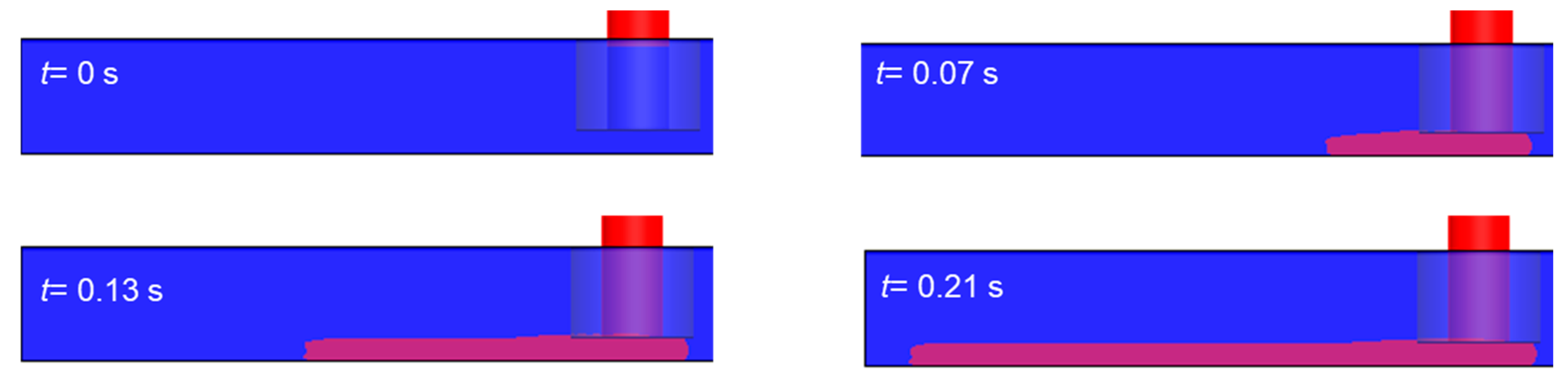
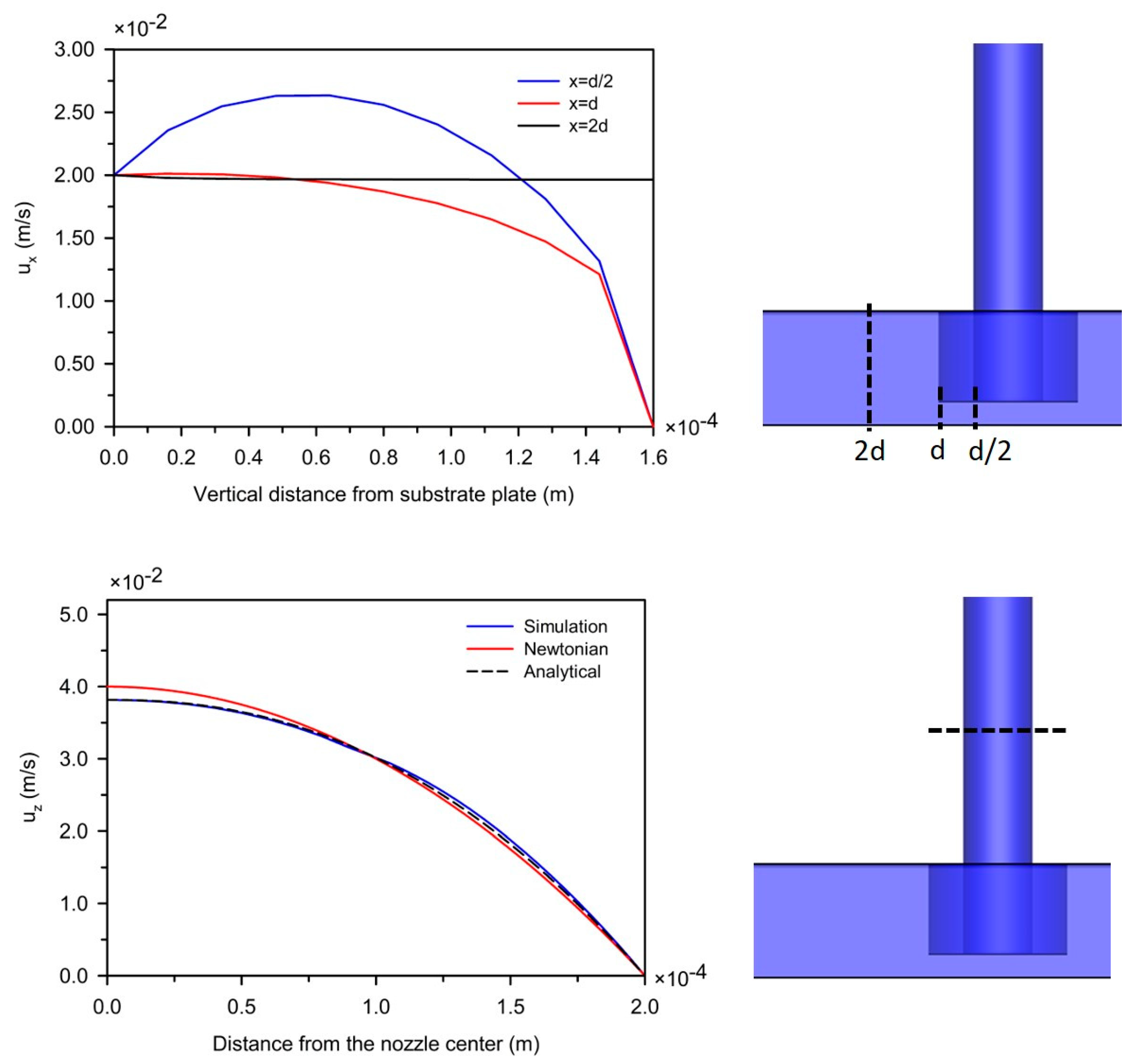
3.1. Simulation of the Extrusion Process

The process where a PLA melt is extruded through the nozzle and deposited on the substrate surface is simulated in this procedure, as described in Section 2. The simulated time-evolution of the liquid fraction (α ≥ 0.5: red) is presented in Figure 4. Note that the color fraction 0 ≤ α < 0.5 is set to the atmosphere (blue). This color definition of each phase gives a clear surface contour to compare to the actual shape of the PLA melt flow [15]. At t = 0, a PLA melt in the nozzle with T = 473 K (for atmosphere, T = 298 K) starts flowing out of the nozzle. As time lapses, the PLA melt is extruded with <u> = 0.02 m/s and subsequently is being deposited along the substrate surface which is moving at U = 0.02 m/s.
Figure 5 presents the simulation results of the velocity magnitude distributions in the extruded strand as well as in the nozzle under the same condition as Figure 4. In Figure 5 (top), as the extruded liquid is deposited away from the nozzle, the velocity distribution in the deposition flow becomes almost uniform due to the free surface effect (the stress on the liquid surface becomes negligibly small). This transition of the flow pattern in the moving substrate direction indicates that a shear rate dependent property, such as the shear thinning viscosity, is dominant near the nozzle but becomes weaker in the deposition flow. The flow in the nozzle behaves like a pressure-driven flow in a cylinder which has the centerline velocity close to 2<u> of a Newtonian fluid and a maximum shear rate on the inner nozzle surface (Figure 5 bottom). The simulated velocity profile also shows good agreement with the corresponding analytical expression for a power-law fluid.
Figure 6 presents the simulated temperature distribution of an extruded strand under the same condition in Figure 4 and Figure 5. As soon as the hot melt in the nozzle (473 K) is extruded through the nozzle, it is exposed to the colder atmosphere (298 K), and its temperature distribution becomes non-uniform indicating that the temperature-dependent viscosity has also changed.
Figure 7 shows the viscosity distribution in the extruded strand. As shown in Figure 6 and Figure 7, the non-uniform temperature distribution directly affects the viscosity distribution which is expected to affect the flow behavior in the strand and the strand shape [8].

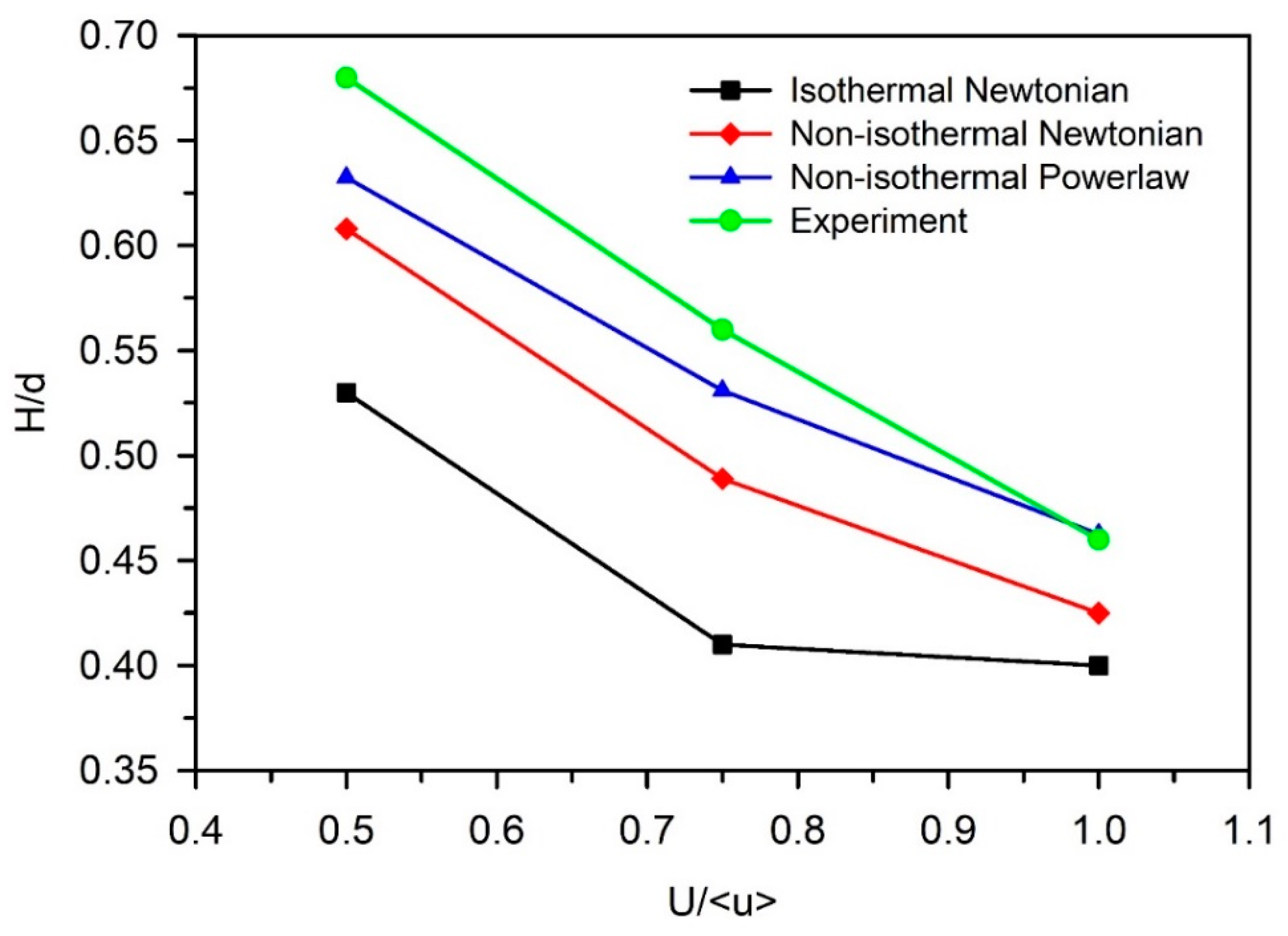
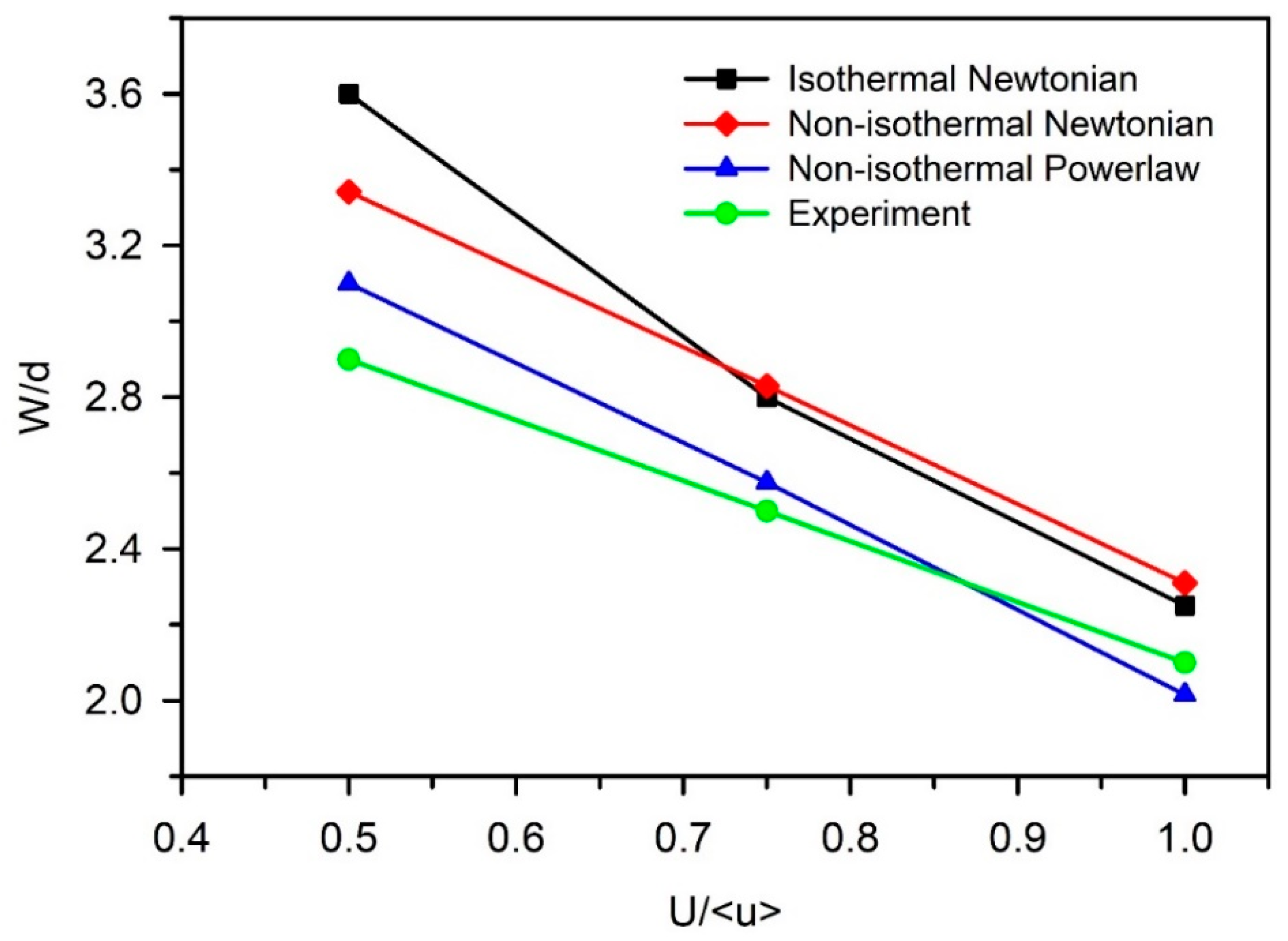
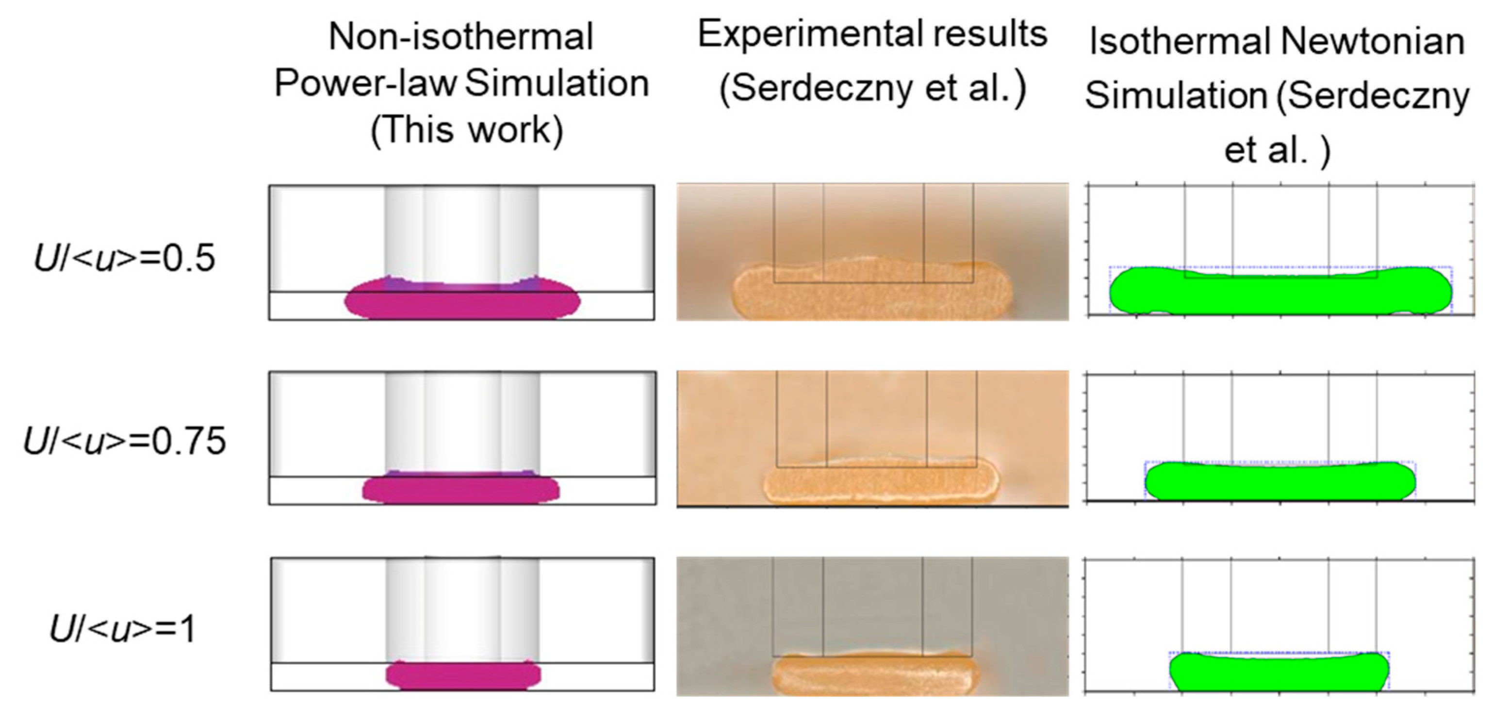
3.2. The Effect of the Viscosity Model on the Relation between Strand Shape and U/<u>

Serdeczny et al. [15] studied the relation between the strand shape and the process conditions. They experimentally measured the width, W, and the thickness, H, of a strand extruded with various conditions of g/d and U/<u>. Their CFD simulation assumed the polymer melt to be an isothermal Newtonian fluid and was able to match the experimentally observed relation for a large gap of g/d = 1. However, it showed a discrepancy for a smaller gap, g/d = 0.4. We hypothesized that the discrepancy is due to the non-uniform viscosity and investigated the strand shape and U/<u> for g/d = 0.4 using our numerical model based on a non-isothermal power-law fluid. As demonstrated in Figure 8, W and H are measured at the cross-section of the liquid fraction of an extruded strand (at x = d).
Figure 9 shows the relations between H/d and U/<u> obtained from various simulation methods and the study by Serdeczny et al. [15]. The overall qualitative trend is that H/d decreases with increasing U/<u> (as U gets slower than <u>, the strand becomes thicker). The result from the isothermal Newtonian simulation (with the same approach as Comminal et al. [14] and Serdeczny et al. [15]) shows the largest quantitative discrepancy from the experimental data. However, the result from our non-isothermal simulations show improved agreement with the experimental data. The non-isothermal power law simulation results in the smallest discrepancy from the experiment. We also performed a non-isothermal Newtonian simulation (set n = 1 in Equation (3)) for comparison. The improvement by the non-isothermal Newtonian simulation is not as much as that of the non-isothermal power-law simulation.
Figure 10 shows the relationship between W/d and U/<u> obtained from the same simulations and experiments as Figure 9. Again, our non-isothermal power-law simulation shows the most improved agreement with the experimental data and the non-isothermal Newtonian simulation results in limited improvement. The differences shown in Figure 9 and Figure 10 according to different models indicate that both the effect of temperature and shear rate contributes to the strand shape. As shown in Figure 5, Figure 6 and Figure 7, the temperature and the velocity profiles in the extruded strand are non-uniform, which affects the viscosity, resulting in the shape of the cross section. Figure 5 (top) showed that the shear rate in the strand diminishes along the distance from the nozzle. However, the formation of the cross-sectional shape happens mainly near the nozzle where the liquid fraction has higher fluidity and shear rate than the deposited part away from the nozzle.
Figure 11 directly compares the cross-sections of an extruded strand obtained from various simulations and experiment. The cross-section obtained from the isothermal Newtonian simulation is wider than the experimental measurement and this work’s simulation. This can be explained by considering the temperature and viscosity profiles seen in Figure 6 and Figure 7. The surface of a strand has a lower temperature and higher viscosity than its inside. The exterior’s higher viscosity has low fluidity which limits the spreading of the strand. Therefore, the width should be smaller than that of the isothermal Newtonian simulation where a constant viscosity of 1000 Pa⋅s is imposed. We believethat the quantitative agreement with the experimental data is improved because the temperature-dependent power law viscosity model is fitted to the experimental data measured from the PLA commonly used in the FDM, and the time step size is properly adjusted to handle very high viscosity. However, there still remains the quantitative discrepancy from the experimental data. Direct experimental measurement rather than using data from literature as well as including viscoelasticity is expected to be able to improve the quantitative agreement [29].

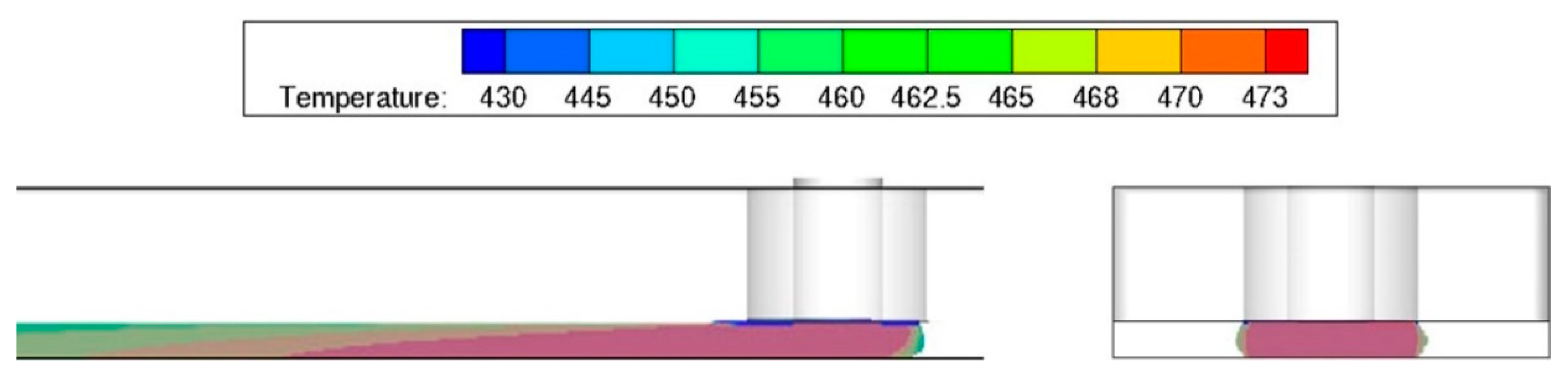
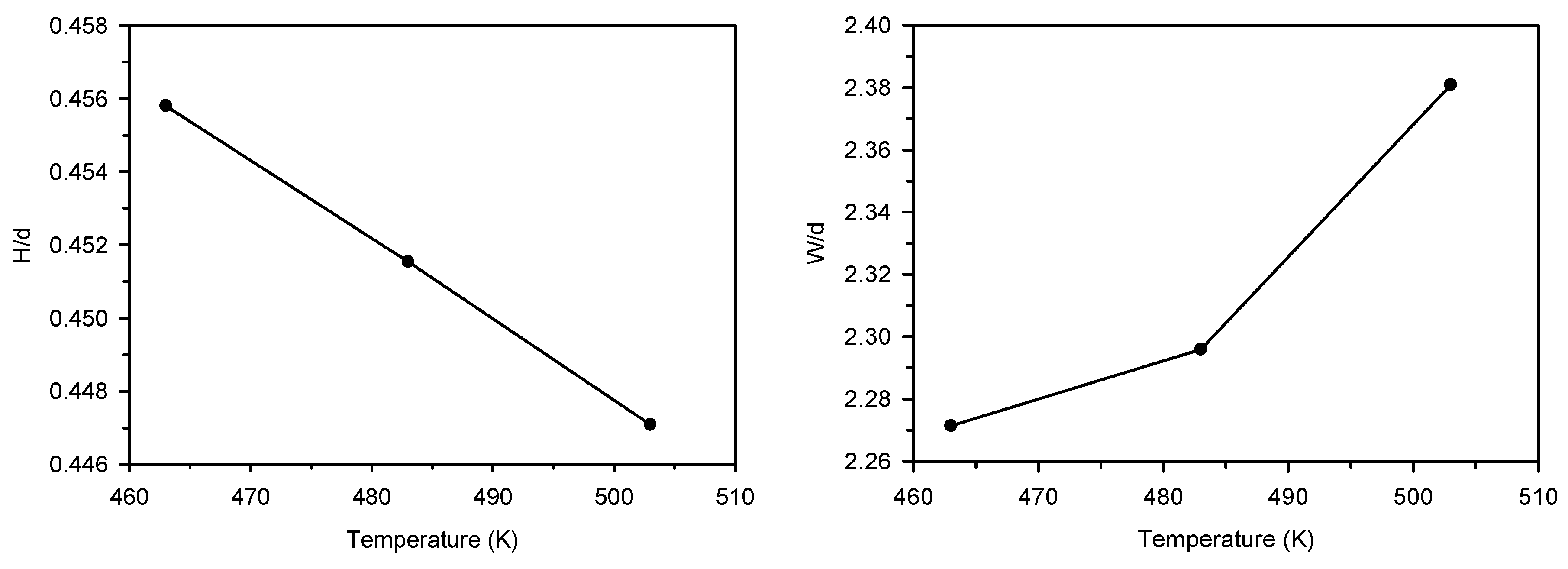
3.3. The Effect of the Nozzle Temperature on the Strand Shape

As shown in the previous section, the temperature is an important factor in accurately modeling the strand shape. We performed the simulation with different temperatures of the PLA in the nozzle to learn more of the temperature effect on the strand shape. Figure 12 shows the strand height and width obtained from the simulation with three different nozzle temperatures and a processing condition of g/d = 0.4 and U/<u> = 1. As the temperature increases, H/d decreases and W/d increases. The polymer flow inside the nozzle has the assigned temperature. As it is extruded into the air and onto the substrate surface, the flow is cooled to the ambient temperature (298 K in this simulation) and the viscosity significantly rises. Higher fluid temperatures in the nozzle result in a higher temperature and a lower viscosity of the deposited fluid which spreads more (larger W/d) resulting in a wider strand. Since the cross-sectional area of the strand must remain constant, H/d shows the opposite trend.

3.4. The Effect of the Nozzle Temperature on the Strand Uniformity

One of the problems of FDM is due to the surface roughness of the final product [30]. The process requires a finalizing stage so that resolution of the final product meets customers’ expectations. One of the reasons for the surface roughness of the final product is the non-uniformity of layers. In other words, the thickness and width of the final product is not constant and changes along the layers. In previous studies, layer uniformity had been adjusted by introducing additives [31,32,33,34]. One study also considered the temperature effect on the strand uniformity: the surface roughness of the final product is reduced with increasing nozzle temperature [34]. We performed a simulation using our numerical model to investigate the temperature effect on surface uniformity. Figure 13 shows a simulation result of the strand width change along the strand axis (distance from the nozzle) with three different fluid temperatures in the nozzle.
The results show the width becomes more uniform with higher temperatures. Standard deviations at each temperature are measured as 0.144, 0.0635, and 0.0319 mm for 463, 483, and 503 K, respectively. Our simulation can show the relation of surface uniformity and nozzle temperature similar to the experimental observation in [34]. This observation can be explained by the viscosity–temperature relationship discussed in the previous sections. Higher temperatures in the nozzle lead to a more fluidic material being deposited on the substrate. This fluid will spread more and has a larger chance of obtaining a uniform surface before cooling to the point of solid-like viscosity. Although our current model can show the temperature-dependent uniformity, there are many rheological factors to be considered in the extrusion process in FDM for controlling the surface properties. For example, shark skin and die swelling are attributed to viscoelasticity and affect the surface uniformity of printed products [26]. Therefore, the addition of viscoelasticity to the numerical model will be the next step in further investigation.

4. Conclusions

We used OpenFOAM to simulate the extrusion process of FDM considering the temperature and shear-dependent viscosity which was fitted from experimental data. We compared our simulated strand shape extruded under a small gap condition and straight nozzle with published experimental data under the same conditions. The comparison showed that temperature-dependent viscosity is effective in improving the agreement with experimental observation: As the surface of the extruded strand becomes cooler, the higher viscosity surface hinders the strand from spreading across the substrate which is not observed in the isothermal Newtonian simulation. The parametric studies with various nozzle temperatures also showed that non-isothermal flow behavior is significant in strand shape and surface uniformity: The less viscous liquid portion with the higher nozzle temperature makes the extruded strand spread more across the substrate with a higher strand uniformity.
In our particular choice of geometry and process, due to the comparison with the available published data, the temperature and shear rate-dependent viscosity model was the major contribution to the improved prediction of extruded strand shape. The addition of viscoelasticity to the numerical model is ongoing for further improving its fit to experimental data and its predictive capabilities in other geometries and processes, such as welding of extruded strands.

Author Contributions

Conceptualization, J.P.; methodology, B.B.; software, B.B.; validation, B.B. and J.P.; formal analysis, B.B.; investigation, B.B., M.S., and J.P.; resources, L.M.; data curation, B.B.; writing—original draft preparation, B.B.; writing—review and editing, M.S., L.M., M.L. and J.P.; visualization, B.B.; supervision, M.L. and J.P.; project administration, M.L. and J.P.; funding acquisition, M.L. and J.P. All authors have read and agreed to the published version of the manuscript.

Funding

This work was funded by the Intellectual Systems Center at the Missouri University of Science and Technology.

Conflicts of Interest

The authors declare no conflict of interest. The funders had no role in the design of the study; in the collection, analyses, or interpretation of data; in the writing of the manuscript, or in the decision to publish the results.

Appendix A

The ability of the new solver to calculate the temperature distribution in multiphase fluids was validated by comparing the results of a simple benchmark simulation using COMSOL Multiphysics, a popular commercial CFD software. For the benchmark simulation, a two-phase system with transient heat transfer was chosen. Detailed geometry of the two-phase system is depicted in Figure A1. The liquid phase is a hypothesized material with ρ = 800 kg/m3, η = 0.002 Pa⋅s, cp = 1800 J/kg⋅K and k = 13 W/m⋅K. The temperature of the entire system was initially set to T = 298 K. At t ≥ 0, all the wall temperatures are maintained at 298 K except the wall at the bottom of the liquid domain which was set to 500 K. The gas phase is set as air with 1 atm. Dimensionless temperature was defined as:
θ = T 298 500 298
Dimensionless temperature distribution in the liquid as a function of the distance from the bottom wall is plotted for both COMSOL and OpenFOAM at t = 1 min (Figure A2). Figure A2 shows that the simulation results from both OpenFOAM and COMSOL are almost identical. Therefore, we deemed our model valid for describing the heat transfer in the open surface flow problems.
Figure A1. Schematic of a benchmark two-phase system for validating our new module.
Jmmp 04 00046 g0a1
Figure A2. Dimensionless temperature profile along the axis (distance from the bottom wall) resulting from the calculations using OpenFOAM with our new module (TempInterFoam) as well as COMSOL Multiphysics.
Jmmp 04 00046 g0a2

References

  1. Horn, T.J.; Harrysson, O.L.A. Overview of current additive manufacturing technologies and selected applications. Sci. Prog. 2012, 95, 255–282. [Google Scholar] [CrossRef] [PubMed]
  2. Pourali, M.; Peterson, A.M. Thermal Modeling of Material Extrusion Additive Manufacturing. In Polymer-Based Additive Manufacturing: Recent Developments; ACS Publications: Washington, DC, USA, 2019; pp. 115–130. [Google Scholar]
  3. Gilmer, E.L.; Mansfield, C.; Gardner, J.M.; Siochi, E.J.; Baird, D.G.; Bortner, M.J. Characterization and Analysis of Polyetherimide: Realizing Practical Challenges of Modeling the Extrusion-Based Additive Manufacturing Process. In Polymer-Based Additive Manufacturing: Recent Developments; ACS Publications: Washington, DC, USA, 2019; pp. 69–84. [Google Scholar]
  4. Garg, A.; Tai, K.; Savalani, M. State-of-the-art in empirical modelling of rapid prototyping processes. Rapid Prototyp. J. 2014, 20, 164–178. [Google Scholar] [CrossRef]
  5. Bellini, A. Fused Deposition of Ceramics: A Comprehensive Experimental, Analytical and Computational Study of Material Behavior, Fabrication Process and Equipment Design. Ph.D. Thesis, Drexel University, Philadelphia, PA, USA, 2002. [Google Scholar]
  6. Brenken, B.; Barocio, E.; Favaloro, A.J.; Kunc, V.; Pipes, R.B. Development and validation of extrusion deposition additive manufacturing process simulations. Addit. Manuf. 2019, 25, 218–226. [Google Scholar] [CrossRef]
  7. D’Amico, T.; Peterson, A.M. An adaptable FEA simulation of material extrusion additive manufacturing heat transfer in 3D. Addit. Manuf. 2018, 21, 422–430. [Google Scholar] [CrossRef]
  8. Cuan-Urquizo, E.; Barocio, E.; Tejada-Ortigoza, V.; Pipes, R.B.; Rodriguez, C.; Roman-Flores, A. Characterization of the Mechanical Properties of FFF Structures and Materials: A Review on the Experimental, Computational and Theoretical Approaches. Materials 2019, 12, 895. [Google Scholar] [CrossRef] [Green Version]
  9. Huang, B.; Singamneni, S. Adaptive slicing and speed- and time-dependent consolidation mechanisms in fused deposition modeling. Proc. Inst. Mech. Eng. Part B J. Eng. Manuf. 2013, 228, 111–126. [Google Scholar] [CrossRef]
  10. Huang, B.; Singamneni, S. Raster angle mechanics in fused deposition modelling. J. Compos. Mater. 2014, 49, 363–383. [Google Scholar] [CrossRef]
  11. Ramanath, H.S.; Chua, C.K.; Leong, K.F.; Shah, K.D. Melt flow behaviour of poly-ε-caprolactone in fused deposition modelling. J. Mater. Sci. Mater. Electron. 2007, 19, 2541–2550. [Google Scholar] [CrossRef]
  12. Mostafa, N.; Syed, H.M.; Igor, S.; Andrew, G. A study of melt flow analysis of an ABS-Iron composite in fused deposition modelling process. Tsinghua Sci. Technol. 2009, 14, 29–37. [Google Scholar] [CrossRef]
  13. Heller, B.; Smith, D.E.; Jack, D.A. Effects of extrudate swell and nozzle geometry on fiber orientation in Fused Filament Fabrication nozzle flow. Addit. Manuf. 2016, 12, 252–264. [Google Scholar] [CrossRef]
  14. Comminal, R.; Serdeczny, M.P.; Pedersen, D.B.; Spangenberg, J. Numerical modeling of the strand deposition flow in extrusion-based additive manufacturing. Addit. Manuf. 2018, 20, 68–76. [Google Scholar] [CrossRef] [Green Version]
  15. Serdeczny, M.P.; Comminal, R.; Pedersen, D.B.; Spangenberg, J. Experimental validation of a numerical model for the strand shape in material extrusion additive manufacturing. Addit. Manuf. 2018, 24, 145–153. [Google Scholar] [CrossRef]
  16. Santana, L.; Alves, J.L.; Netto, A.D.C.S. A study of parametric calibration for low cost 3D printing: Seeking improvement in dimensional quality. Mater. Des. 2017, 135, 159–172. [Google Scholar] [CrossRef]
  17. Bartikian, M.; Ferreira, A.; Gonçalves-Ferreira, A.; Neto, L.L. 3D printing anatomical models of head bones. Surg. Radiol. Anat. 2018, 41, 1205–1209. [Google Scholar] [CrossRef] [PubMed]
  18. Zhang, Y.; Chou, K. A parametric study of part distortions in fused deposition modelling using three-dimensional finite element analysis. Proc. Inst. Mech. Eng. Part B J. Eng. Manuf. 2008, 222, 959–968. [Google Scholar] [CrossRef]
  19. Rosas, L.F.V. Characterization of Parametric Internal Structures for Components Built by Fused Deposition Modeling. Master’s Thesis, University of Windsor, Windsor, ON, Canada, 2013. [Google Scholar]
  20. Dabiri, S.; Schmid, S.; Tryggvason, G. Fully Resolved Numerical Simulations of Fused Deposition Modeling. In Proceedings of the ASME 2014 International Manufacturing Science and Engineering Conference collocated with the JSME 2014 International Conference on Materials and Processing and the 42nd North American Manufacturing Research Conference, Detroit, MI, USA, 9–13 June 2014. [Google Scholar] [CrossRef]
  21. McIlroy, C.; Olmsted, P.D. Deformation of an amorphous polymer during the fused-filament-fabrication method for additive manufacturing. J. Rheol. 2017, 61, 379–397. [Google Scholar] [CrossRef] [Green Version]
  22. Liu, J.; Anderson, K.L.; Sridhar, N. Direct Simulation of Polymer Fused Deposition Modeling (FDM)—An Implementation of the Multi-Phase Viscoelastic Solver in OpenFOAM. Int. J. Comput. Methods 2019, 17, 1844002. [Google Scholar] [CrossRef] [Green Version]
  23. Xia, H.; Lu, J.; Tryggvason, G. A numerical study of the effect of viscoelastic stresses in fused filament fabrication. Comput. Methods Appl. Mech. Eng. 2019, 346, 242–259. [Google Scholar] [CrossRef]
  24. Phan, D.D.; Swain, Z.R.; Mackay, M.E. Rheological and heat transfer effects in fused filament fabrication. J. Rheol. 2018, 62, 1097–1107. [Google Scholar] [CrossRef]
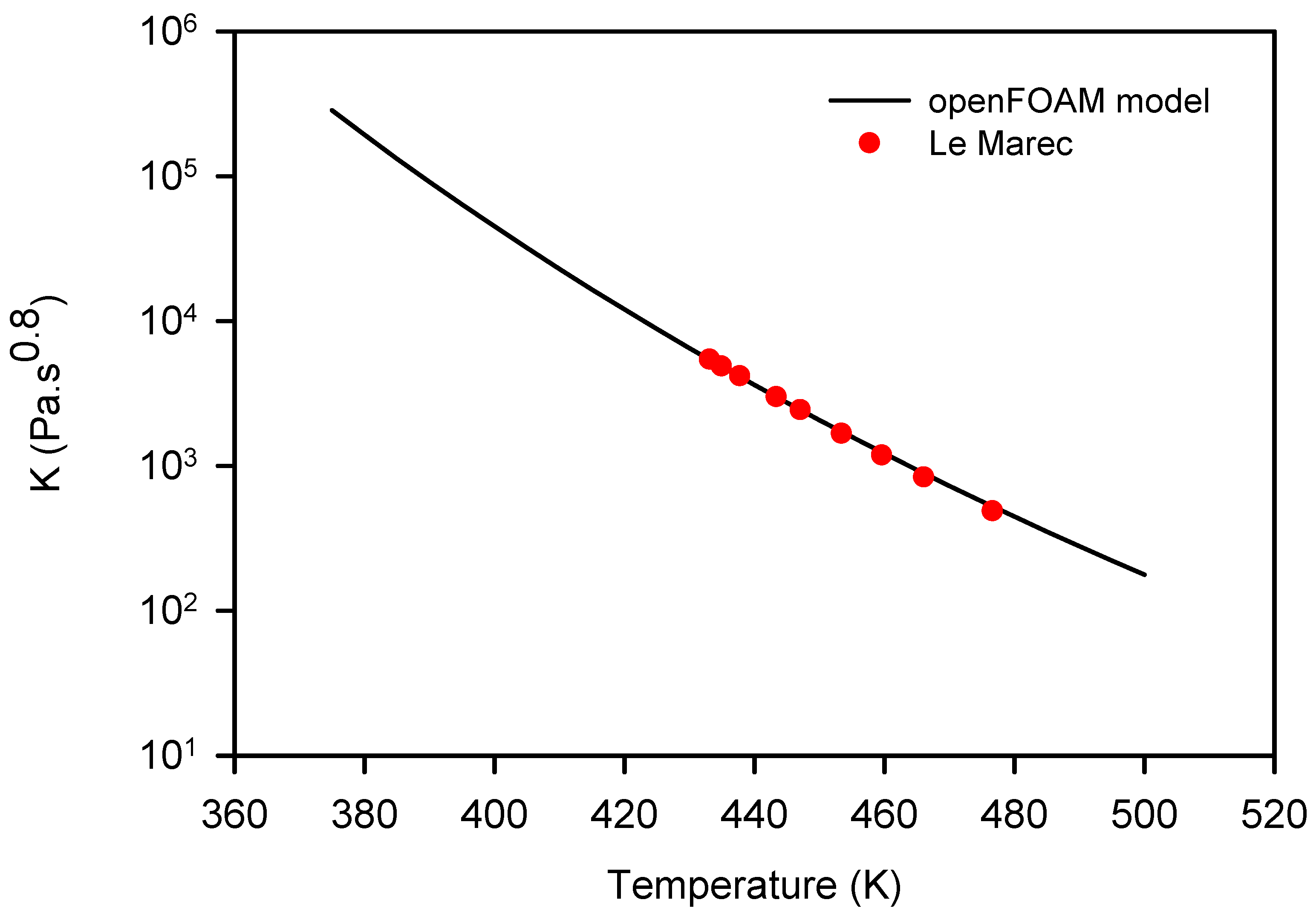
  25. Le Marec, P.E.; Quantin, J.-C.; Ferry, L.; Benezet, J.-C.; Guilbert, S.; Bergeret, A. Modelling of PLA melt rheology and batch mixing energy balance. Eur. Polym. J. 2014, 60, 273–285. [Google Scholar] [CrossRef]
  26. Mackay, M.E. The importance of rheological behavior in the additive manufacturing technique material extrusion. J. Rheol. 2018, 62, 1549–1561. [Google Scholar] [CrossRef]
  27. Deshpande, S.S.; Anumolu, L.; Trujillo, M.F. Evaluating the performance of the two-phase flow solver interFoam. Comput. Sci. Discov. 2012, 5, 014016. [Google Scholar] [CrossRef]
  28. Larsen, B.E.; Fuhrman, D.R.; Roenby, J. Performance of interFoam on the simulation of progressive waves. arXiv 2018, arXiv:1804.01158. [Google Scholar] [CrossRef] [Green Version]
  29. Comminal, R.B.; Hattel, J.H.; Spangenberg, J. Numerical simulations of planar extrusion and fused filament fabrication of non-Newtonian fluids. Nord. Rheol. Soc. Annu. Trans. 2017, 25, 263–270. [Google Scholar]
  30. Turner, B.N.; Strong, R.; Gold, S.A. A review of melt extrusion additive manufacturing processes: I. Process design and modeling. Rapid Prototyp. J. 2014, 20, 192–204. [Google Scholar] [CrossRef]
  31. Ang, T.; Sultana, F.; Hutmacher, D.W.; Wong, Y.; Fuh, J.; Mo, X.; Loh, H.; Burdet, E.; Teoh, S. Fabrication of 3D chitosan–hydroxyapatite scaffolds using a robotic dispensing system. Mater. Sci. Eng. C 2002, 20, 35–42. [Google Scholar] [CrossRef]
  32. Trachtenberg, J.; Placone, J.K.; Smith, B.T.; Fisher, J.P.; Mikos, A.G. Extrusion-based 3D printing of poly(propylene fumarate) scaffolds with hydroxyapatite gradients. J. Biomater. Sci. Polym. Ed. 2017, 28, 532–554. [Google Scholar] [CrossRef] [Green Version]
  33. Jamróz, W.; Kurek, M.; Łyszczarz, E.; Szafraniec-Szczęsny, J.; Knapik-Kowalczuk, J.; Syrek, K.; Paluch, M.; Jachowicz, R. 3D printed orodispersible films with Aripiprazole. Int. J. Pharm. 2017, 533, 413–420. [Google Scholar] [CrossRef]
  34. Chaidas, D.; Kitsakis, K.; Kechagias, J.; Maropoulos, S. The impact of temperature changing on surface roughness of FFF process. IOP Conf. Ser. Mater. Sci. Eng. 2016, 161, 12033. [Google Scholar] [CrossRef] [Green Version]
Figure 1. Schematic of the simulated system: nozzle and a substrate plate. The flow in the nozzle is in the z-direction. The substrate is moving in the x-direction.
Jmmp 04 00046 g001
Figure 2. Discretization of the simulated system using hexahedral meshes.
Jmmp 04 00046 g002
Figure 3. K vs. T by fitting the experimental data from Le Marec et al. [25] to Equation (4).
Jmmp 04 00046 g003
Figure 4. Time evolution of the PLA melt extrusion process: The melt flow is visualized by showing α ≥ 0.5 as red color. The surrounding atmosphere (0 ≤ α < 0.5) is represented as blue.
Jmmp 04 00046 g004
Figure 5. The distributions of a velocity component: (Top) the x-component of u, ux, in the strand flow from our simulation and (Bottom) the z-components of u, uz, inside the nozzle, evaluated from Newtonian model, analytical calculation of Equation (3), and our simulation The dash lines in each offset image show the location where the velocity component distributions were obtained.
Jmmp 04 00046 g005
Figure 6. Temperature profile in an extruded strand (U/<u> = 1, nozzle temperature = 473 K).
Jmmp 04 00046 g006
Figure 7. Kinematic viscosity distribution of an extruded strand (U/<u> = 1, nozzle temperature = 473 K).
Jmmp 04 00046 g007
Figure 8. A liquid fraction of a simulated extruded strand in xy-plane and demonstration of how W and H of the cross section is made.
Jmmp 04 00046 g008
Figure 9. Comparison of H/d vs. U/<u> for g/d = 0.4 obtained from simulations and the experiment. Isothermal Newtonian simulation results are from Serdeczny et al. [15] which we were able to reproduce using our model. (Lines connecting symbols are for visual guidance).
Jmmp 04 00046 g009
Figure 10. Comparison of W/d vs. U/<u> for g/d = 0.4 obtained from simulations and the experiment. (Lines connecting symbols are for visual guidance).
Jmmp 04 00046 g010
Figure 11. Comparison of the cross-sections obtained from simulations and experiment (The images were adapted from Serdeczny et al. [15] by permission from Elsevier).
Jmmp 04 00046 g011
Figure 12. The effect of nozzle temperature on H/d (Left) and W/d (Right) of strands obtained from simulation (g/d = 0.4 and U/<u> = 1). (Lines connecting symbols are for visual guidance).
Jmmp 04 00046 g012
Figure 13. Widths of a strand along X (distance from the nozzle) with different nozzle temperatures. (Lines connecting symbols are for visual guidance).
Jmmp 04 00046 g013

