
A Study of the Convective Cooling of Large Industrial Billets


School of Metallurgy & Materials, University of Birmingham, Edgbaston, Birmingham B15 2TT, UK
J. Manuf. Mater. Process. 2021, 5(4), 137; https://doi.org/10.3390/jmmp5040137
Submission received: 3 November 2021
/
Revised: 10 December 2021
/
Accepted: 14 December 2021
/
Published: 16 December 2021
Abstract
:The thermodynamic heat-transfer mechanisms, which occur as a heated billet cools in an air environment, are of clear importance in determining the rate at which a heated billet cools. However, in finite element modelling simulations, the convective heat transfer term of the heat transfer mechanisms is often reduced to simplified or guessed constants, whereas thermal conductivity and radiative emissivity are entered as detailed temperature dependent functions. As such, in both natural and forced convection environments, the fundamental physical relationships for the Nusselt number, Reynolds number, Raleigh parameter, and Grashof parameter were consulted and combined to form a fundamental relationship for the natural convective heat transfer as a temperature-dependent function. This function was calculated using values for air as found in the literature. These functions were then applied within an FE framework for a simple billet cooling model, compared against FE predictions with constant convective coefficient, and further compared with experimental data for a real steel billet cooling. The modified, temperature-dependent convective transfer coefficient displayed an improved prediction of the cooling curves in the majority of experiments, although on occasion a constant value model also produced very similar predicted cooling curves. Finally, a grain growth kinetics numerical model was implemented in order to predict how different convective models influence grain size and, as such, mechanical properties. The resulting findings could offer improved cooling rate predictions for all types of FE models for metal forming and heat treatment operations.
1. Introduction
The industrially focused processing of bulk metal forming, and the associated manufacturing operations such as open-die and closed-die forging, played a significant role in global industrialisation and subsequent manufacturing growth and development [1]. Whilst forging methods and techniques have developed to allow for smaller, more intricate forging objects to be accurately formed through the process, similarly the development of hydraulic presses and very large forging hammers has, in parallel, driven the use of forging techniques to manufacture huge forgings for very heavy industry, weighing an excess of 50 tonnes. The use of various steels as the primary material for structural use has dominated the global metals industry for over a century, largely due to its superior materials properties, the abundance of iron, and the cost efficiency of manufacture [2]. By alloying with additional elements including vanadium, nickel, molybdenum, chromium, cobalt, and others, in small quantities, specialised alloy steels, for specific purposes, can be produced [3], ranging from corrosion resistant stainless steels to the ultra-hard tool steels. Steel manufacture globally in 2020 was 1.88 × 10⁹ tonnes, with China manufacturing more than 50% [4].
Structural steel is a class of steel alloys that are commonly used within the construction industry but also within industries including aerospace, power generation, nuclear, and marine industries. Structural steels are commonly produced in specific shapes including beams, bars, and general billets, allowing for more complex shaping of the raw material by using machining or bulk forming operations [5], such as press forging and drop-forging. Forged components and forged billets are prevalent within the industry because of the inherent strength attained through refined grain structure [6]. The largest forgings are commonly used for heavy industries, including marine, nuclear, and power generation. Large forging presses can have in excess of 20,000 tonnes of press force, whilst drop hammer forges can have drop-hammers in excess of 1500 tonnes with a drop height of 5 metres or greater.
Open-die forging methods are often utilised to process very large billets, which consists of a series of hammer blows or press stages used to change the dimensions of the billet. As with all hot-forging operations, the heat transfer to surroundings and heat loss from the heated billet is of important consideration. Hot forging operations require the billet to be pre-heated to forging temperature by using induction [7] or furnace heating [8] methods. However, due to the considerable mass of these large industrial steel billets, the heating costs account for the considerable production cost [9]. As such, it becomes important to understand the rate at which these billets cool for a number of reasons: firstly, to reduce the number of reheating processes by forging the heated billet soon after exiting the heating stage; secondly, to understand post-forging cooling time, as the large billets will take up considerable floor space as they cool and require significant separation from one another to cool without influencing and reheating one another. Thus, this can present a bottleneck to the process—once available space runs out—as the cooling time for very large billets is considerable.
Numerous research has considered the cooling of large billets previously. Borisov and Goland [10] measured cooling rates for a cylindrical 550 mm diameter billet from different tempering temperatures and with different atmospheric conditions including natural convection and forced convection. They concluded with a series of design rules for water flow rate to yield different microstructures. Ma et al. [11] considered fundamental physics to produce a numerical framework to model the heat transfer coefficient for a spray cooled casting. Whilst Maisuradze et al. [12] measured overall heat transfer coefficients for large steel forgings with a spray-cooling environment. Rasouli et al. [13] studied the effects that cooling rate plays upon the microstructure and subsequent properties of steel billets, with cooling rates varying from 3 to 15 °C/s. They summarised further design rules for required cooling rate to achieve the following: (i) high strength but with reduced ductility or (ii) increased toughness.
Similarly, Pola et al. [14] investigated spray cooling, for a heavy 26NiCrMoV 11.5 steel billet, using experiment and finite element modelling to determine the role that the water pressure within the jets, as well as the flow rate, plays during quenching, noting that water pressure had little influence on the cooling of larger sections, albeit some significance in thinner sections. Whilst water flow rate had a small but noticeable impact, Lacarac et al. [15] experimentally and computationally with fluid dynamics (CFD) measured cooling rates to back-calculate using the inverse method the overall heat transfer coefficients on different surfaces at different incident angles compared to air cross-flow current during a forced convective cooling environment. They concluded that heat transfer coefficients can be a factor of three in the same system for different incident angled surfaces.
As such, the intention of this work is to use fundamental fluid dynamics dimensionless parameters, thermo-physical properties, and thermodynamic relationships to allow for an improved understanding of the significance of the convective heat transfer mechanism and to estimate heat transfer coefficients based upon these fundamental principles. These data would prove useful to industries involved in the processing and manufacture of large blank billets. A methodology of carrying forward the fundamental fluid dynamics data to a quick-to-compute finite element modelling framework, considering a simple geometry billet cooling, will be presented, and thermal predictions from FE are compared against experimental work within the literature. This framework will allow heavy industry, smaller companies, and process engineers to simulate the influence of the convective heat transfer term upon the evolving materials properties, including grain size and yield strength, with minimal simplifications considered.
2. Mathematical Theory
2.1. Fundamental Heat Transfer Mechanisms
Heat transfer mechanisms during the cooling of a component fall within three distinct thermodynamic mechanisms: conduction, convection, and thermal radiation. Conduction is primarily a solid material heat transfer; thus, conduction dictates the heat transfer within a heated solid steel billet. In its simplest 1D form, it can be expressed using Fourier’s Law given in Equation (1):
whereby q is the local heat flux density (W·m−2), k the thermal conductivity (W·m−1·K−1), and the thermal gradient (W·m−1). Thus, as the exterior cools, the hotter interior transfers heat, via thermal conductivity, through the solid. Convection and thermal radiation are heat exchange mechanisms between the surface of the solid object and the surroundings. Thus, these two mechanisms drive surface cooling initially. Convection can additionally be expressed in an overall heat exchange equation, along with thermal conductivity, as given in Equation (2), whereby U is the effective (overall) heat transfer coefficient, hc is convective heat transfer coefficient (W·m−2·K−1), and dxw is the part thickness. However, this relationship does not include cooling caused by thermal radiation.
Thermal radiation/emissivity is a thermodynamic heat transfer mechanism which is always present, regardless of whether there is any atmospheric media. However, at low temperatures it contributes a very small cooling term compared to convective currents. On the other hand, at high temperatures, particularly as the component begins to glow with the heat, emissivity becomes the dominant heat transfer mechanism. Thermal radiation for a grey-body (with emissivity less than 1) can be described by the Stefan–Boltzmann equation given in Equation (3):
whereby j is the energy flux (W·m−2), T is temperature in K, ε the emissivity (0 < ε < 1), and σ is the Stefan–Boltzmann constant, (5.67 × 10⁻⁸ W·m−2·K−4). Whilst both the thermal conductivity, k, and the thermal radiation (emissivity), ε, are material properties of the solid billet that is cooling, the convection term, hc, is a “system” property, and it is dependent upon atmospheric temperature and atmospheric conditions including air speed/agitation. The material properties (thermal conductivity and emissivity) can be measured directly using methods such as Transient hot wire, Lee’s disc, or the laser flash method or tables can be consulted for accurate material data, the convective transfer coefficient h is a much more uncertain value.
Currently, when cooling in an air atmosphere, the available research [16] provides some guidance as to the value of the parameter h for thermal convection heat transfer, but these proposed values (see Table 1) have relatively wide intervals for different atmospheric conditions. Thus, it becomes of interest to utilise fundamental equations that can allow for the estimation of the natural convective coefficient as a function of temperature.
2.2. Derivation of Dimensionless Parameters
By considering convective heat transfer from fundamental principles, certain dimensionless parameters are commonly used as fluid and heat transfer characteristics. These arise from dimensional analysis using the Buckingham Pi Theorem and Rayleigh’s method of dimensional analysis [18]. By formulating a dimensionless term Π as a function of the known physical parameters associated with fluid flow, each raised to an unknown power defined by an arbitrary letter, and solving for the arising set of simultaneous equations when performing a dimensional balance, the dimensionless Π-groups are yielded. These are given in Equation (4), for Nusselt number, Equation (5), for Reynolds number, and Equation (6) for Prandtl number:
whereby all the dimensionless Π-groups are related by Nusselt’s expression [19] given in Equation (7):
whereby V is velocity, µ is dynamic viscosity and ν is kinematic viscosity, ρ is density, L is characteristic length, k is thermal conductivity, hc is the convective coefficient, and cp is the specific heat capacity. The scaling parameter C and powers α and β are values to be determined by the geometry and conditions of the system. From Nusselt’s expression given in Equation (7), specific values of the three parameters α, β, and C have been defined in differing systems to yield the well-known empirically derived Dittus–Boelter equations, the Sieder and Tate correlation, and the Hausen expression [20].
By using similar Buckingham Pi dimensional analysis activities considering the buoyancy force per unit volume, one can again derive the Prandtl and Nusselt numbers, as well as a dimensionless value called the Grashof number (Gr) [17], which is formally a product of the remaining two Π-groups formed. The Grashof number is defined in Equation (8):
whereby g is gravitational acceleration, β is thermal expansion coefficient, ΔT is temperature difference between the surface and locations far away from the object, atmospheric (initial) temperature was 20 °C, L is a characteristic length, and ν is kinematic viscosity.
The Rayleigh number for a fluid flow was formulated by using a combination of the dimensionless Grashof and Prandtl numbers. It describes a ratio of the time-scales for heat loss via conduction to the time-scales for heat loss via convection, and the case for natural convection is presented in Equation (9):
which is commonly simplified by using the standard definitions of viscosity (Equation (10)):
and the thermal diffusivity term (Equation (11)):
to yield the Rayleigh number (Equation (12)).
At this point, one must consider the magnitude of the Grashof, Rayleigh, and Reynolds numbers in order to determine whether the air-flow displays laminar or turbulent behaviour. For vertical plates, which will be a close match to the geometry considered here, the assumed cut-off for laminar to turbulent behaviour for the Rayleigh number is 109 [17]. Given that for the geometry considered here, the Rayleigh number calculated actually spans this value of 109 at lower and higher air temperatures; thus, makes a selection of the parameters for general Equation (13) [17] challenging.
Alternatively, work on proposing an entire range approximation, by Churchill and Chu [20], yields the empirically derived expression given in Equation (14).
2.3. Natural Convection
In order to calculate the natural convective heat transfer terms, one can use temperature-dependent values in the literature [21] for ν and k. Subsequently, by using a constant thermal expansion (0.0032 K−1) and g = 9.81 m·s−2, temperature dependent tabular calculations for all the required dimensionless parameters—namely the Prandtl, Grashof, Rayleigh, and Nusselt numbers—and the arising natural convective heat transfer coefficient h, based upon the Churchill and Chu model, are computed and provided in Table 2. Note that this first principle calculation using the assumed expressions for Rayleigh, Grashof, and Nusselt, which are only valid for certain conditions, yields a room temperature convective coefficient of approximately 3.0 to 3.3 W·m−2·K−1 within the widely quoted range of permissible convective transfer coefficients in a natural convection system. This value is right at the bottom of the permissible range, suggesting that this calculation is in line with others’ work, albeit potentially with a high degree of conservatism.
2.4. Forced Convection
In addition to the fundamental derivation of values for natural convection in air, it is also of great interest to understand how much effect any additional external mechanisms such as fans or air currents have upon the increase in the convective coefficient, when moving in to a forced convection regime. Thus, the engineer can again revert back to the fundamental dimensionless properties used to define and describe air flow systems. Whilst the Reynolds number (Equation (5)) was of little use for natural convection systems considered before, due to its dependence upon air velocity, this parameter now becomes highly useful for a forced convective system. Within a vertical cylinder experiment, the Sieder and Tate correlation (Equation (15)) is used:
where µ and µs are the dynamic viscosity of air at bulk and cooling surface temperatures. Thus, one can apply the Sieder and Tate correlation of the Nusselt number and, thus calculate a temperature dependent function for hc using temperature-dependent density of air, temperature dependent dynamic viscosity of air at the surface temperature (880 °C) and a cold air value (1.8 × 10⁻⁵ kg·m−1·s−1), temperature dependent thermal conductivity, and the characteristic length as the cylinder radius. This calculation yields a temperature dependent forced convective coefficient hc dependent upon the air speed, as provided in Figure 1. Again, the calculated forced convective heat transfer coefficient was in excellent agreement with the data quoted in Table 1, particularly the values from Incropera [17].
3. FE Modelling Methodology
Computational fluid dynamics (CFD) models are typically used to simulate air flow across different geometries given the suitability of these software for fluid mechanics problems. However, for industrial companies producing the large billets, the greater desire is to understand what role this plays within the solid component, given that this is their manufacturing output. Thus, finite element (FE) software is suitable for calculating both heat transfer effects and the linked metallurgical effects within a solid mechanics system. Whilst CFD software would generate greater accuracy, an FE approach is considered more likely to be adopted by industrial forging companies due to existing skillsets within forging and metal forming industry. It has the additional benefit of the coupled thermal-metallurgical functionality and is likely a computationally cheaper method, with the earlier described fundamentally derived fluid mechanics relationships embedded as temperature-dependent heat transfer functions within the FE code.
The geometry considered in experimental work by Borisov and Goland [10] was replicated in this work to compare FE thermal predictions using the theory developed here against experimental data. As such, a 0.55 m diameter, 1.6 m tall billet was constructed within FE software Deform (v11.3) using the 2D axisymmetric mode (with 2D axi-symmetric element type) to allow for the most efficient computation of the problem. The FE modelling setup is shown in Figure 2. The model made a simplification that there was no supporting floor for the billet; thus, it did not lose any negligible amount of heat through conduction with a floor. The initial air temperature was set at 20 °C, with surface transfer coefficient calculated using the arithmetic mean of the bulk and surface temperatures [19].
The FE model was ran as a purely thermal-metallurgical analysis, with a constant time step of 10 s and a mesh element length varying between 5 mm and 18 mm (graded with finer elements at the surface). The model employed a representative material model for the 35KhN3MFA rotor steel, which has a chemical composition as stated in the literature [22] and is presented in Table 3, with density constant at 7900 kg·m−3. An emissivity constant to simulate the thermal radiative cooling of the part within the FE model of 0.75 was included in to the model, and thermal conductivity and specific heat capacity were included as temperature-dependent functions as given in Figure 3.
The convection coefficient was defined in a number of ways, firstly as a constant value commonly used in FE modelling and secondly as a temperature-dependent function, using the fundamentally derived values for natural and forced convection conditions developed in the theoretical work. All other modelling parameters and values were constant; thus, it allowed a direct study of the effect that the convective term particularly had upon the cooling rates of large steel billets, with an experimentally measured cooling curve for validation. For the forced cooling experiment, a forced air convective transfer term based upon the Sieder and Tate correlation for a moderate air flow speed of approximately 40 to 50 m/s was assumed, in absence of any firm data in the experiment.
The effects of buoyancy forces, which may result in a variation in the Nusselt number across the height of the cylinder, have currently been ignored for the sake of computational simplicity. The height of the cylinder considered in the Borisov and Goland work [10] compared to its diameter is a ratio of roughly 3:1; thus, by ignoring this term, the results are a slight simplification of the true fluid dynamics involved, and as such the model will produce largely uniform thermal profiles, with the exception for edge effects, which is a simplified prediction compared to the more accurate results from a CFD software.
4. Results
The FE models were simulated on a 16Gb RAM desktop workstation, with simulation time of approximately 1 h. After simulation, the models were interrogated for cooling rates at nodes representative of (a) the middle of the billet and (b) a node at the mid-height point on the outer wall of the billet. Furthermore, the results from the various simulations were compared against experimental data. Screenshots from the FE models for the naturally cooling 2D axisymmetric billet are given in Figure 4 in order to highlight how thermal fields are evolving during cooling and also to illustrate the overall similarities between evolving thermal fields from the fixed and temperature-dependent functions for convective heat transfer.
The subtle differences in the modelled cooling rates require further analysis at relevant nodes (matching the experimental thermocouple locations) to display trends in a more concise manner. It becomes evident when further analysing the cooling rates at specific nodes either at the centre, or the outer edge of the billet, that small variations in cooling rates are predicted by the different convection coefficients over the duration of the FE simulation. Using the Borisov and Gorland [10] experimental data as validation, the graphs presented in Figure 5a illustrate that for the natural cooling experiment, the FE model using the temperature-dependent function improved the match compared to the experiment for the measurement taken on the outer edge.
However, this improvement only really becomes evident after approximately 7 h of cooling, whereby the temperature dependent function for hc shows a fractionally hotter billet at the centre matched by a fractionally cooler billet at the edge by roughly 30 °C. Thus, the temperature dependence of the convective term marginally affects the rate at which heat is lost from the surface and, in turn, influences the rate at which heat rebalances in the part through conduction.
It is noted that both models were not particularly accurate at predicting the initial significant cooling rate on the exterior edge over approximately the first 5 h. However, the experimental data and the prediction converged again at approximately the 10 h mark and produced a good final prediction. The discrepancies in the predicted cooling rate compared to experiment could be due to experimental issues, including thermocouple tip contact with the sample and thermal lag in the thermocouple. However, it is also potentially a real trend that the simplified heat loss terms, using the standard FE assumptions (including (i) the assumed convective transfer coefficients computed and (ii) the constant radiative heat loss term), and the impact of ignoring the variation in Nusselt caused by buoyancy effects has not been represented accurately within the model.
The forced convective cooling FE model predictions and experimental validation data are presented in Figure 5b, and the predictions for the forced cooling model using the temperature dependent convective term are again an improvement upon the model using a fixed hc value. The temperature dependent hc value shows significantly better matching to both the centre and edge temperatures in the 2 to 7 h time period, albeit with a 30 to 40 °C error. On the other hand, the fixed hc model cools too rapidly at the start of this time interval. For both locations, the temperature-dependent hc model does marginally match better to the experimental temperature after 10 h plus of cooling, although these differences are minimal. However, it must also be stated that the reasonably good matching of the temperature-dependent hc model may be due to the modeller being able to freely choose the “air-speed” hc function to match experimental data. Given that the historical experimental data from the literature included no air-speed for the forced cooling condition, the best-matching dataset was employed.
5. Discussion
Understanding the cooling curves experienced by metallic components more accurately has numerous industrial benefits. It can allow for alleviation of process-route bottlenecks, such as being able to reduce required cooling times for large components. It allows for scheduling pre-forging heating operations or forging blows such that new components or parts are released from the prior manufacturing stage to the subsequent manufacturing operation and, finally, to cooling the holding pen in order to coincide with other parts that are exiting.
However, an improved understanding of cooling curves also has metallurgical and mechanical benefits. The cooling rate is one of the principal influences on grain size, which in turn strongly influences the mechanical properties such as yield strength, toughness and hardness. Given the successful validation activity on the cooling rates at different locations within the billet, the use of the FE model is extended, and this time it is extended in an unvalidated form in order to make further predictions for metallurgical and microstructural trends and to predict grain growth within the FE model. As such, a well-established phenomenological solution of a parabolic form, presented in the literature by Semiatin [23], has been employed. In this approach, the mean grain size is allowed to grow with the relationship, as provided in Equation (16):
where d is final grain size (μm), d0 is the starting grain size (μm), t is time (s), Q is the activation energy for grain growth (J/mol), R is the universal gas constant (8.314 J·mol−1·K−1), T is temperature (in Kelvin), and A and n material-specific constants. The grain growth model was applied to the billet during cooling from 880 °C, with an assumed initial grain size of 2.5 µm throughout the billet. Literature [24,25,26] were consulted to find appropriate values for the activation energy and material constants for a low-to-medium carbon steel with relatively low manganese content, with values used matching or close to these estimates, with activation energy Q = 400 kJ·mol−1, kinetic exponent, n = 6, and scaling parameter A = 1.8 × 1023 µm6·s−1.
The arising grain growth predictions from FE showed negligible sensitivity to the type of convective law used (either constant convective heat transfer coefficient, or a temperature dependent parameter), and these predictions of grain growth for the natural convection and forced convection billets are given in Figure 6. They also showed only very minor variation from one another, with all the grain growth kinetics occurring within the first hour of cooling. In fact, the vast majority of that occurred within the first 30 min of the cooling period. The largest grains at the slow cooling centre in the natural convective cooling model reached 17.8 µm in diameter. On the other hand, the smallest grains at the surface only reached 8.2 µm. For the forced convective cooling model, the central, slower cooling region reached an average grain size of 17.1 µm in diameter, whilst the more rapidly cooling grains at the edge only reached 7.3 µm. This would strongly suggest that this initial short period of the cooling process is by far the most critical for influencing grain size and, in turn, the mechanical properties of the cooling billet. It, therefore, highlights a very narrow window of time for the industry to concentrate on controlling billet cooling rate and temperature and to optimise the final properties of the material.
The Hall–Petch relationship (see Equation (17)) governs the yield strength of the material as a function of the average grain size. This emerging yield strength, σY, is dependent upon the average grain size, d, and the material constants, k and σ0.
The material constants σ0 and k are assumed to be 400 MPa and 530 MPa·µm0.5 [27], respectively. The FE model predicts that the largest grains—on the axisymmetric centreline of the billet—increased to approximately 17.1 to 17.8 µm (depending on the convection being wither forced or natural), whereas the smallest grains, at the outer edge of the billet, only increased approximately 7.4 to 8.2 µm (see Table 4). Thus, the Hall–Petch relationship would suggest that the material at the centre of the billet has a yield strength of 528 MPa, whilst the material at the edge of the billet has a strength of 596 MPa. Thus, the centre of the cooled billet, due to the grain growth kinetics, has become slightly less strong than the finer grained outer edge by approximately 15%.
6. Conclusions
A temperature-dependent function for describing the convective heat transfer coefficient between a heated billet and the atmosphere, for both natural and forced convection, has been constructed by using fundamental properties of air-flow including thermal conductivity, air velocity, dynamic and kinematic viscosity and density, forming the Reynolds, Rayleigh, Grashof, and Prandtl numbers. These tabular datasets were used in an FE model to compare cooling curve predictions against a constant convective coefficient model and against the experiment. The following conclusions were drawn:
- A fundamental calculation of natural convective heat transfer using known empirical relationships which are valid for certain conditions produces a room temperature hc value of approximately 3 W·m−2·K−1 at the bottom-end of the usual quoted range of hc values for air. This ranged up to 9 W·m−2·K−1 at elevated temperatures and plateaued at temperatures above 700 °C due to the effects of increasing kinematic viscosity cancelling with the effects of increasing conductivity.
- The FE analysis for the natural convective cooling shows that the cooling rate at the edge for the temperature dependent hc term matches the experiment marginally better than for fixed cooling, although both models matched one another for the first 7 h. For the centre location during natural convective cooling, the FE prediction matched to experimental measurements was a little more wayward during the first 4 h.
- For the forced convective cooling case, varying the hc term in the FE models produced a more noticeable effect, with the edge node cooling curve matching the result from FE with temperature dependent hc function reasonably well. Similarly, for the centre node, results for the temperature dependent hc term were an improved fit to the experiment compared to fixed hc.
- The validated thermal model was extended to include metallurgical effects. Grain size kinetics were predicted to show that there were negligible effects on the arising grain size for different convective term models. Even a comparison of natural versus forced convective cooling showed only very minor grain size variation. The dominant grain size pattern is for the centre to have coarser grains due to slower cooling, and the edge region grains are smaller due to more rapid cooling. This is present in all grain size FE predictions.
- Thus, the convective heat transfer term is concluded to be only of minor importance to metallurgical features, with a small window of opportunity at the start of the cooling phase, during which the cooling rate dominates the arising grain size and mechanical properties of the material.
Author Contributions
Conceptualization, methodology, software, formal analysis, writing (all), R.T. All authors have read and agreed to the published version of the manuscript.
Funding
This research received no external funding.
Data Availability Statement
The data presented in this study are available on request from the corresponding author. The data are not publicly available due to file size limitations.
Acknowledgments
Many thanks to colleagues in the School of Metallurgy and Materials at the University of Birmingham for the support and advice offered during the work. Thanks to Wilde Analysis (Stockport, UK) and to Wilde Analysis staff James Farrar and Tomas Brownsmith for their technical support with the Deform FE software.
Conflicts of Interest
The authors declare no conflict of interest.
References
- Groche, P.; Fittshe, D.; Tekkaya, E.A.; Allwood, J.M.; Hirt, G.; Neugebauer, R. Incremental Bulk Forming. Ann. CIRP 2007, 55, 636. [Google Scholar]
- Liu, Q.; Cho, J.-W.; Pereloma, E. Editorial: Advances in Steel Manufacturing and Processing. Front. Mater. 2021, 8, 201. [Google Scholar] [CrossRef]
- Lucacci, G. Materials for Ultra-Supercritical and Advanced Ultra-Supercritical Power Plants—Ch. 7: Steels and Alloys for Turbine Blades in Ultra-Supercritical Power Plants; Woodhead Publishing: Cambridge, UK, 2017. [Google Scholar]
- World Steel Association—Press Release. 2021. Available online: https://www.worldsteel.org/media-centre/press-releases/2021/Global-crude-steel-output-decreases-by-0.9--in-2020.html (accessed on 12 August 2021).
- Black, J.T.; Kohser, R.A. DeGarmo’s Materials and Processes in Manufacturing, 12th ed.; Wiley & Sons: New York, NY, USA, 2017. [Google Scholar]
- Soleymani, V.; Eghbali, B. Grain Refinement in a Low Carbon Steel through Multidirectional Forging. J. Iron Steel Res. Int. 2012, 19, 74–78. [Google Scholar] [CrossRef]
- Rudnev, V.; Loveless, D.; Cook, R.L. Handbook of Induction Heating; CRC Press: Boca Raton, FL, USA, 2017. [Google Scholar]
- Chakravarty, K.; Kumar, S. Increase in energy efficiency of a steel billet reheating furnace by heat balance study and process improvement. Energy Rep. 2020, 6, 343–349. [Google Scholar] [CrossRef]
- Thakur, P.K.; Prakash, K.; Muralidharan, K.G.; Bahl, V.; Das, S. A review on: Efficient energy optimization in reheating furnaces, Int. J. Mech. Prod. Eng. 2015, 3, 18–24. [Google Scholar]
- Borisov, I.A.; Goland, L.F. Cooling large forgings in a water-air mixture. Met. Sci. Heat Treat. 1988, 10, 17–22. [Google Scholar] [CrossRef]
- Ma, H.; Silaen, A.; Zhou, C. Numerical Development of Heat Transfer Coefficient Correlation for Spray Cooling in Continuous Casting. Front. Mater. 2020, 7, 397. [Google Scholar] [CrossRef]
- Maisuradze, M.; Yudin, Y.V.; Ryzhkov, M.A. Investigation and Development of Spray Cooling Device for Heat Treatment of Large Steel Forgings. Mater. Perform. Charact. 2014, 3, 449–462. [Google Scholar] [CrossRef]
- Rasouli, D.; Asl, S.K.; Akbarzadeh, A.; Daneshi, G. Effect of cooling rate on the microstructure and mechanical properties of microalloyed forging steel. J. Mater. Process. Technol. 2008, 206, 92–98. [Google Scholar] [CrossRef]
- Pola, A.; Gelfi, M.; La Vecchia, G. Simulation and validation of spray quenching applied to heavy forgings. J. Mater. Process. Technol. 2013, 213, 2247–2253. [Google Scholar] [CrossRef]
- Lacarac, V.; Smith, D.; McMahon, C.; Tierney, M. Evaluation of non-uniform cooling effects for air-cooled forgings. J. Mater. Process. Technol. 2004, 152, 370–383. [Google Scholar] [CrossRef]
- Kosky, P.; Balmer, R.; Keat, W.; Wise, G. Exploring Engineering—An Introduction to Engineering and Design, 5th ed.; Academic Press: Cambridge, MA, USA. [CrossRef]
- Incropera, F.; Dewitt, D.; Bergmann, T.L.; Lavine, A.S. Principles of Heat and Mass Transfer, 7th ed.; Wiley & Sons: Hoboken, NJ, USA, 2013; ISBN 978-0-470-64615-1. [Google Scholar]
- Buckingham, E. On Physically Similar Systems; Illustrations of the Use of Dimensional Equations. Phys. Rev. 1914, 4, 345–376. [Google Scholar] [CrossRef]
- Brown, A.I.; Marco, S.M. Introduction to Heat Transfer, 3rd ed.; McGraw-Hill Book Company: New York, NY, USA, 1958. [Google Scholar]
- Eckert, E.R.G. Heat and Mass Transfer; McGraw-Hill Book Company: New York, NY, USA, 1959. [Google Scholar]
- Engineers Edge. Viscosity of Air, Dynamic and Kinematic; Engineers Edge LLC: Monroe, GA, USA, 2020; Available online: https://www.engineersedge.com/physics/viscosity_of_air_dynamic_and_kinematic_14483.htm (accessed on 12 August 2021).
- Kramarov, M.A.; Kolchin, G.G.; Lebedev, V.N.; Solntsev, Y.P. Resistance to fracture of steel 35KhN3MFA for large machine parts. Met. Sci. Heat Treat. 1976, 18, 18–20. [Google Scholar] [CrossRef]
- Semiatin, S.; Soper, J.; Sukonnik, I. Short-time beta grain growth kinetics for a conventional titanium alloy. Acta Mater. 1996, 44, 1979–1986. [Google Scholar] [CrossRef]
- Yue, C.; Zhang, L.; Liao, S.; Gao, H. Kinetic Analysis of the Austenite Grain Growth in GCr15 Steel. J. Mater. Eng. Perform. 2010, 19, 112–115. [Google Scholar] [CrossRef] [Green Version]
- Illescas, S.; Fernández, J.; Guilemany, J.M. Kinetic analysis of the austenitic grain growth in HSLA steel with a low carbon content. Mater. Lett. 2008, 62, 3478–3480. [Google Scholar] [CrossRef]
- Giumelli, A. Austenite Grain Growth Kinetics and the Grain Size Distribution. Master’s Thesis, University of British Columbia, Vancouver, BC, Canada, 1995. [Google Scholar]
- Fu, B.; Pei, C.; Pan, H.; Guo, Y.; Fu, L.; Shan, A. Hall-Petch relationship of interstitial-free steel with a wide grain size range processed by asymmetric rolling and subsequent annealing. Mater. Res. Express 2020, 7, 116516. [Google Scholar] [CrossRef]
Figure 1.
Calculated forced convective heat transfer coefficient at range of temperatures.

Figure 2.
Finite element modelling setup.
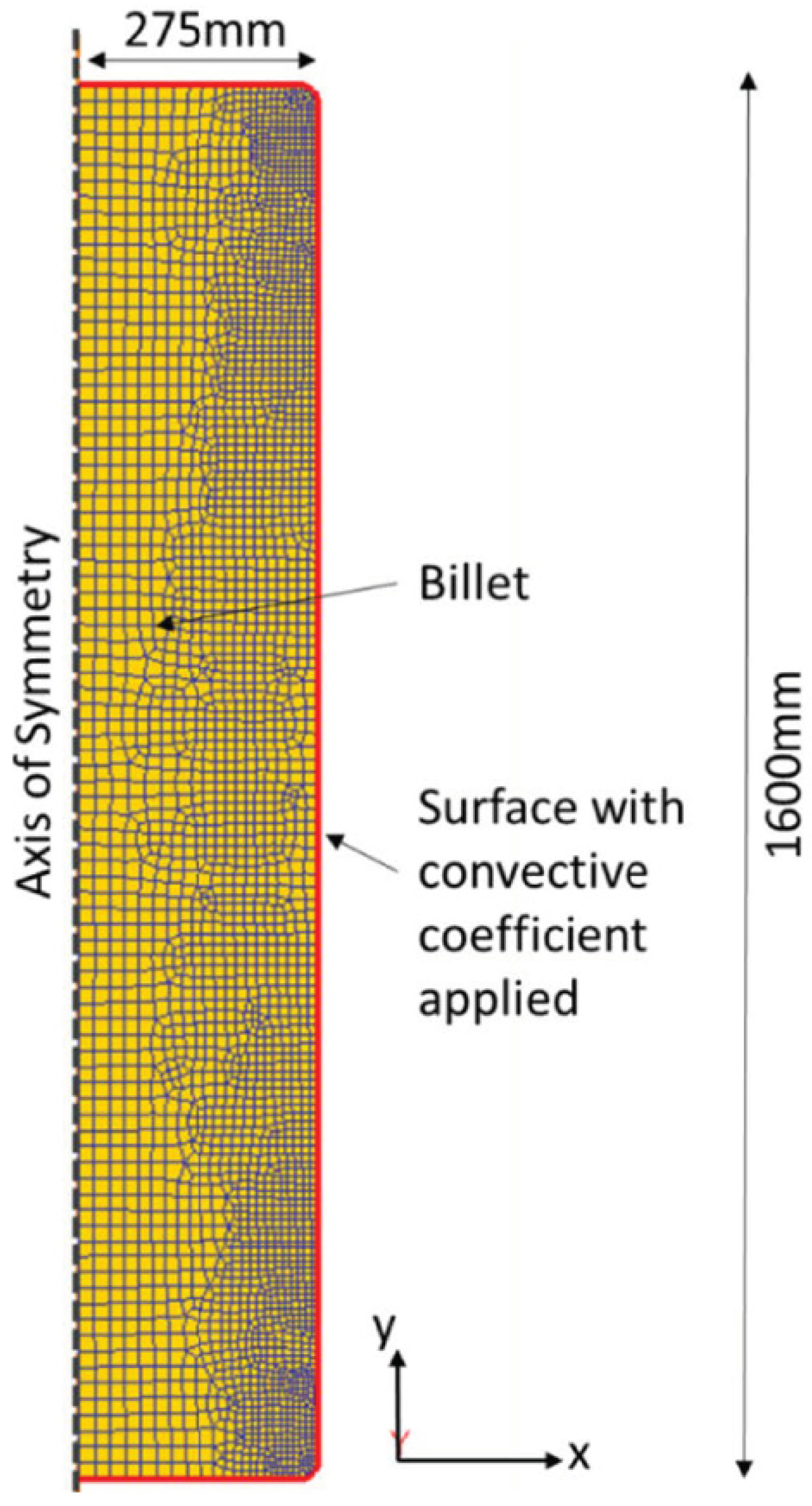
Figure 3.
Thermo-physical properties for the 35KhN3MFA steel used.
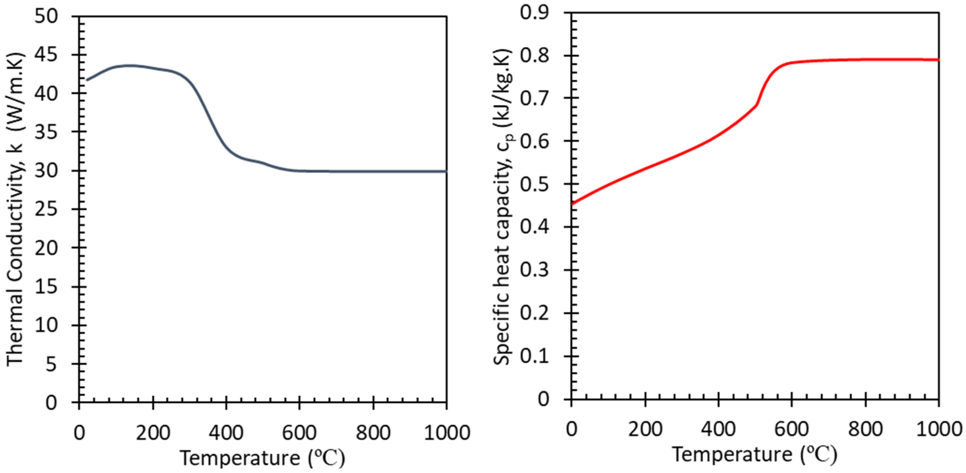
Figure 4.
FE predictions of billet natural cooling after (a) ½ h, (b) 1 h, (c) 2 h, (d) 5 h, and (e) 10 h for (top) constant convection coefficient and (bottom) temperature-dependent convective term.
Figure 4.
FE predictions of billet natural cooling after (a) ½ h, (b) 1 h, (c) 2 h, (d) 5 h, and (e) 10 h for (top) constant convection coefficient and (bottom) temperature-dependent convective term.
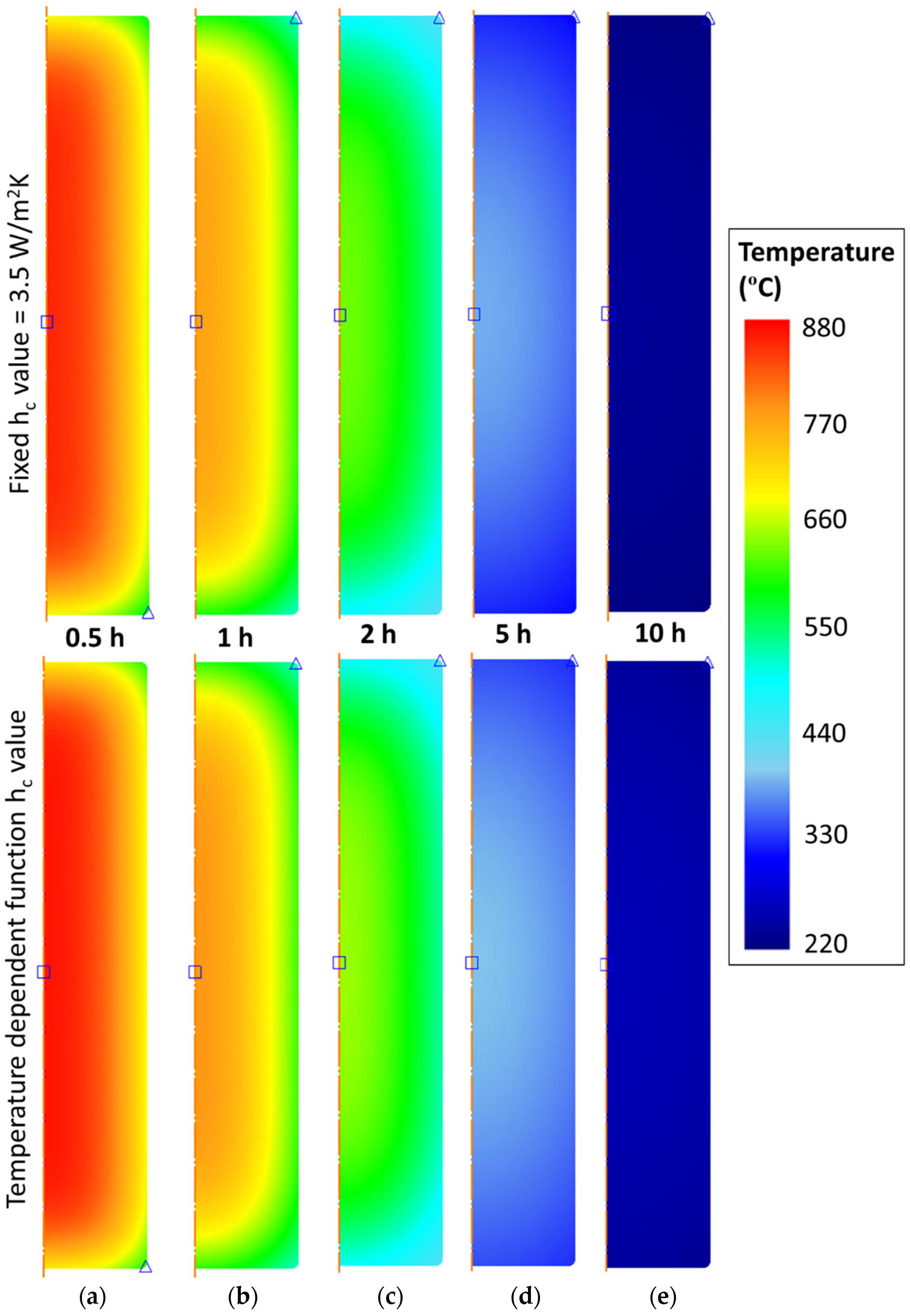
Figure 5.
Cooling curves for (a) naturally cooled billet and (b) forced cooled billet; and for experiment and FE models with constant and a temperature dependent convective heat transfer term.
Figure 5.
Cooling curves for (a) naturally cooled billet and (b) forced cooled billet; and for experiment and FE models with constant and a temperature dependent convective heat transfer term.

Figure 6.
FE prediction of average grain size in natural and forced convective cooled billets.


| Type of Convection | Convective Heat Transfer Coefficient, h (W·m−2·K−1) | |
|---|---|---|
| Kosky et al. [16] | Incropera et al. [17] | |
| Air, natural (free convection) | 2.5 to 25 | 2 to 25 |
| Air, forced convection | 10 to 500 | 25 to 250 |
| Liquids, forced convection | 100 to 15,000 | 100 to 20,000 |
| Boiling water (inc. phase change) | 2500 to 25,000 | 2500 to 100,000 |
Table 2.
Derived thermal conductivity, viscosity, Grashof, Rayleigh, Nusselt numbers and convective coefficient, from first principles, for a range of air temperature.
Table 2.
Derived thermal conductivity, viscosity, Grashof, Rayleigh, Nusselt numbers and convective coefficient, from first principles, for a range of air temperature.
| Temperature (°C) | Thermal Conductivity, k (W·m−1·K−1) | Kinematic Viscosity (m2·s−1) | Prandtl (-) | Grashof (-) | Rayleigh (-) | Nusselt (-) | Convective Coefficient, h (W·m−2·K−1) |
|---|---|---|---|---|---|---|---|
| 25 | 0.026 | 1.64 × 10⁻⁵ | 0.709 | 1.17 × 10⁹ | 8.27 × 10⁸ | 115.84 | 3.01 |
| 30 | 0.026 | 1.68 × 10⁻⁵ | 0.707 | 1.67 × 10⁹ | 1.18 × 10⁹ | 129.17 | 3.36 |
| 40 | 0.027 | 1.70 × 10⁻⁵ | 0.706 | 2.71 × 10⁹ | 1.92 × 10⁹ | 150.13 | 4.05 |
| 50 | 0.027 | 1.80 × 10⁻⁵ | 0.705 | 3.39 × 10⁹ | 2.39 × 10⁹ | 160.78 | 4.34 |
| 100 | 0.031 | 2.30 × 10⁻⁵ | 0.701 | 5.04 × 10⁹ | 3.53 × 10⁹ | 181.54 | 5.63 |
| 200 | 0.038 | 3.40 × 10⁻⁵ | 0.699 | 5.02 × 10⁹ | 3.51 × 10⁹ | 181.07 | 6.88 |
| 300 | 0.044 | 4.70 × 10⁻⁵ | 0.702 | 4.05 × 10⁹ | 2.84 × 10⁹ | 169.61 | 7.46 |
| 400 | 0.05 | 6.20 × 10⁻⁵ | 0.706 | 3.14 × 10⁹ | 2.22 × 10⁹ | 157.14 | 7.86 |
| 500 | 0.055 | 7.80 × 10⁻⁵ | 0.71 | 2.50 × 10⁹ | 1.77 × 10⁹ | 146.74 | 8.07 |
| 700 | 0.066 | 1.10 × 10⁻⁴ | 0.728 | 1.78 × 10⁹ | 1.29 × 10⁹ | 133.46 | 8.80 |
| 1000 | 0.077 | 1.70 × 10⁻⁴ | 0.73 | 1.07 × 10⁹ | 7.80 × 10⁸ | 114.25 | 8.78 |
Table 3.
Chemical composition of rotor steel 35KhN3MFA.
| Element | C | Ni | Cr | Mn | Mo | V | Cu | Si | S | P | Fe |
|---|---|---|---|---|---|---|---|---|---|---|---|
| Wt % | 0.36 | 2.96 | 1.37 | 0.41 | 0.36 | 0.15 | 0.1 | 0.33 | 0.015 | 0.013 | Bal. |
Table 4.
Predicted yield strength of different parts of the billets, for different convective cooling, based upon the Hall–Petch relationship.
Table 4.
Predicted yield strength of different parts of the billets, for different convective cooling, based upon the Hall–Petch relationship.
| Convective Cooling Method | Location in Billet | Grain Size (µm) | Yield Strength (MPa) |
|---|---|---|---|
| Natural convection | Centre | 17.8 | 526 |
| Edge | 8.2 | 585 | |
| Forced convection | Centre | 17.1 | 528 |
| Edge | 7.3 | 596 |
Publisher’s Note: MDPI stays neutral with regard to jurisdictional claims in published maps and institutional affiliations. |
© 2021 by the author. Licensee MDPI, Basel, Switzerland. This article is an open access article distributed under the terms and conditions of the Creative Commons Attribution (CC BY) license (https://creativecommons.org/licenses/by/4.0/).
Share and Cite
MDPI and ACS Style
Turner, R. A Study of the Convective Cooling of Large Industrial Billets. J. Manuf. Mater. Process. 2021, 5, 137. https://doi.org/10.3390/jmmp5040137
AMA Style
Turner R. A Study of the Convective Cooling of Large Industrial Billets. Journal of Manufacturing and Materials Processing. 2021; 5(4):137. https://doi.org/10.3390/jmmp5040137
Chicago/Turabian StyleTurner, Richard. 2021. "A Study of the Convective Cooling of Large Industrial Billets" Journal of Manufacturing and Materials Processing 5, no. 4: 137. https://doi.org/10.3390/jmmp5040137