Predicting Properties of Fused Filament Fabrication Parts through Sensors and Machine Learning

Abstract

Fused filament fabrication (FFF), colloquially known as 3D-printing, has gradually expanded from the laboratory to the industrial and household realms due to its suitability for producing highly customized products with complex geometries. However, it is difficult to evaluate the mechanical performance of samples produced by this method of additive manufacturing (AM) due to the high number of combinations of printing parameters, which have been shown to significantly impact the final structural integrity of the part. This implies that using experimental data attained through destructive testing is not always viable. In this study, predictive models based on the rapid prediction of the required extrusion force and mechanical properties of printed parts are proposed, selecting a subset of the most representative printing parameters during the printing process as the domain of interest. Data obtained from the in-line sensor-equipped 3D printers were used to train several different predictive models. By comparing the coefficient of determination (R²) of the response surface method (RSM) and five different machine learning models, it is found that the support vector regressor (SVR) has the best performance in this data volume case. Ultimately, the ML resources developed in this work can potentially support the application of AM technology in the assessment of part structural integrity through simulation and can also be integrated into a control loop that can pause or even correct a failing print if the expected filament force-speed pairing is trailing outside a tolerance zone stemming from ML predictions.

1. Introduction

The use of additive manufacturing (AM) technologies to produce small batches of highly customized, complex parts in a reduced development cycle is extremely attractive to all industries. For AM parts to be fully adopted in industrial scenarios, engineers have to be able to confidently assess the structural integrity of the finished part under its intended loading conditions. However, the set of printing conditions that lead to an optimal part in terms of mechanical properties are not fully comprehended due to a confluence of two factors: the nuances associated with the interacting effects of the processing conditions and material behavior, paired with a commonplace lack of standardization in the field of AM as a whole.

These challenges present an interesting case for employing different sensors to oversee the additive manufacturing process. Given the pivotal role of melting processing in determining the ultimate performance of specimens produced by Material Extrusion (ME) additive manufacturing, there has been extensive exploration into conducting in-line measurements of temperature and pressure. These measurements aim to establish correlations with shear viscosity [1], interlayer strength [2], and deposition rate [3]. However, when printing at high speeds, the model of melting changes to melting with pressure flow removal [4], and the pressure in the melt region would change significantly at different locations in the nozzle. Therefore, to capture the behavior of both slow and fast printing processes in a more general way, the utilization of force sensors has emerged [5].

Research to explore the effects of different printing parameters on extrusion force and sample mechanical properties through experiments or derivation has never stopped. A comprehensive review [6] underscores the pivotal printing parameters over the mechanical properties of extrusion-based additive manufacturing products, which include raster angle, layer thickness, build orientation, filling ratio, printing speed, printing temperature, and bead width. Notably, Koch’s study proposed product build orientation and the impact of the solidity ratio determined by layer thickness and nozzle diameter on tensile strength [7]. Li’s research showed trends in tensile strength and bonding degree with the increase in printing speed [8]. In the study of extrusion force, the melting model solved by Osswald, etc. shows how nozzle diameter, print speed, and nozzle temperature have an analytical influence on extrusion force [4]. In the computational fluid dynamics (CFD) model, the nozzle diameter plays an important role in the filament feed force under consideration of viscoelasticity [9]. Through experiments, Mazzei Capote, etc. summarized the impact of printing speed on the extrusion force of ABS and PLA at different temperatures [5]. In the pursuit of a balance between the practicality of data collection through experimentation and the reliability inherent in predictive models, our study casts a spotlight on build orientation, layer thickness, nozzle diameter, and printing speed. These parameters serve as the focal points for predicting extrusion force and tensile properties, signifying their paramount importance in the realm of extrusion-based additive manufacturing research.

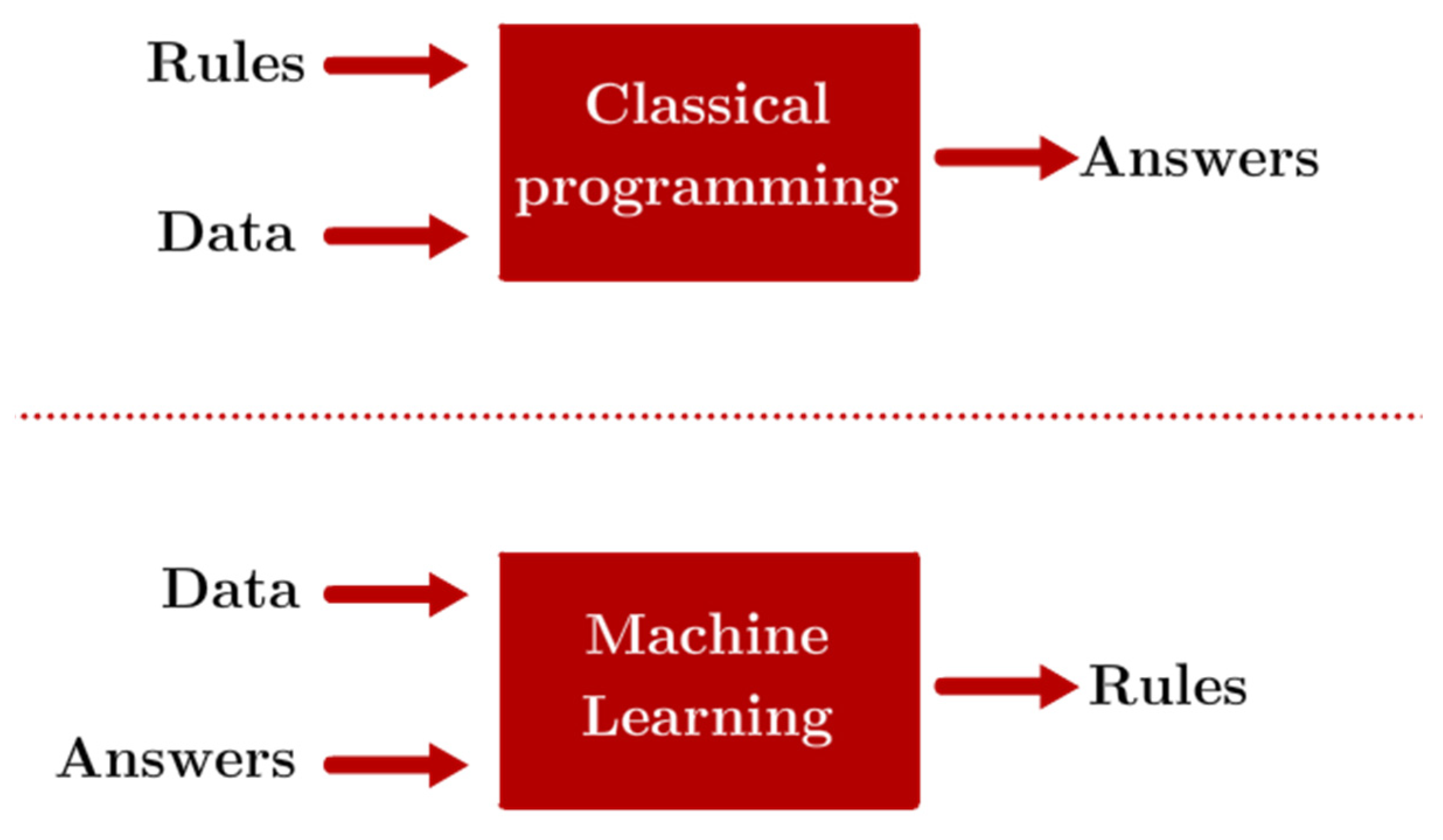
Recent advancements in processing power and algorithms have made it easier than ever to deploy machine learning (ML) solutions, and the intricacies of the processing-properties relationships of AM techniques represent an interesting case for the development of ML algorithms. These excel in cases where the inputs and outcomes of a particular phenomenon or task are known, but connecting the two through an explicit set of rules or relationships can be extremely complex and time-consuming [10]. In this manner, ML models are trained as opposed to explicitly programmed, as illustrated in Figure 1, where the differences between ML and traditional programming philosophies are compared. ML techniques are applicable in situations where the inputs and outputs of a particular phenomenon are known, but there’s a lack of explicit rules that indicate a relationship between the two.

The application of ML in AM can be mainly divided into three directions: printer health state monitoring, part quality detection, and resource management. In health state monitoring of 3D printers, the filament feeding state has been investigated by different sensors with various ML methods for data processing and classification. The feature space reduction and unsupervised cluster center identifications were employed to classify normal, block, semi-block, and run-out of material states [11]. Synthetic acceleration and the back propagation neural network (BPNN) were applied to preprocess the data from vibration sensors and classify normal and filament jam states [12]. Regarding part quality control, both final part performance and layer-wise defect detection were studied. Feed stock characteristics and processing parameters are the main variables for part performance. The combination of two main factors was applied to the prediction of the compressive modulus and shore hardness of PolyJet-printed multi-material anatomical models [13]. In the realm of predicting the mechanical properties of finished parts, Bayraktar et al. [14] generated three mathematical models, corresponding to three different raster patterns, to predict tensile strength (σ_t) by inputting layer thickness and nozzle temperature. However, the network architectures were trained separately for each raster pattern, which is not convenient for mechanical property prediction with varying orientations in a single print. For layer-wise detection, the convolutional neural network used for camera data analysis was applied for depositing defect detection [15], and multiple regression algorithms were compared in surface roughness prediction with mounted infrared temperature sensors and accelerators [16]. Except for product quality, optimization of resource consumption during processing is also important during the evaluation of processing parameters. The potential time, cost, and feedstock quantity were predicted with fuzzy inputs [17].

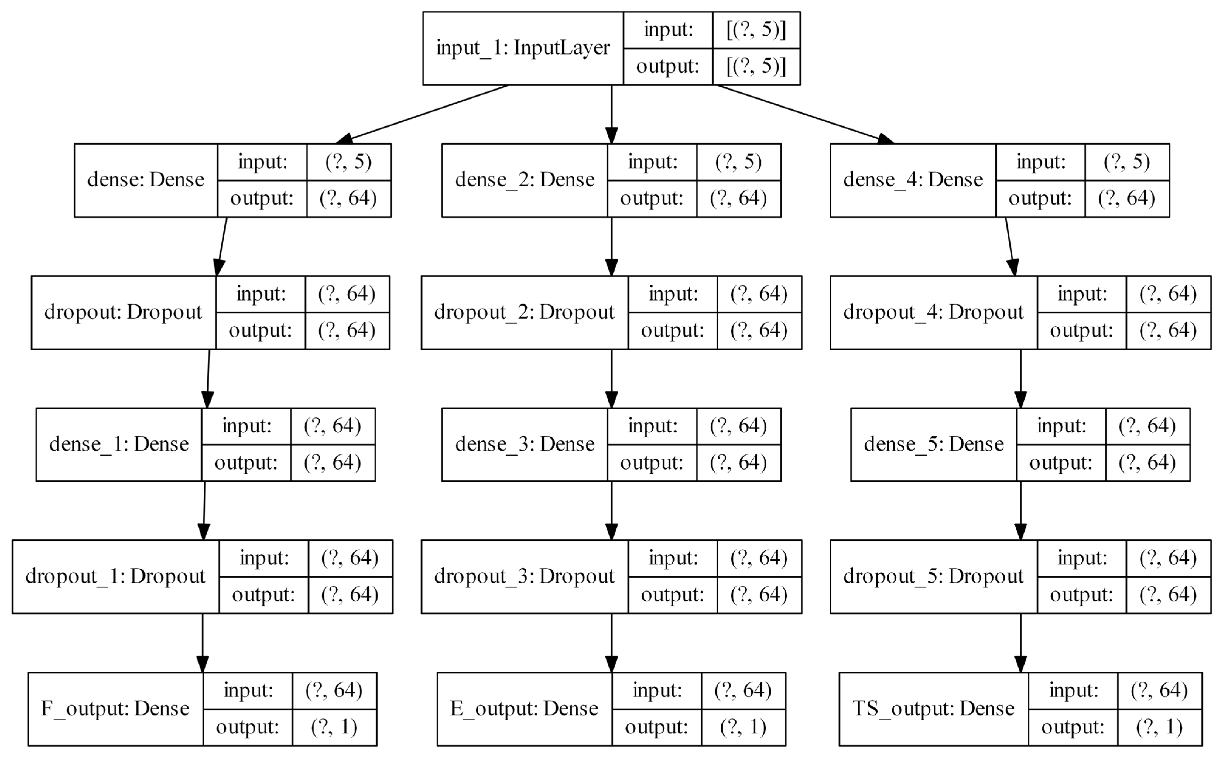
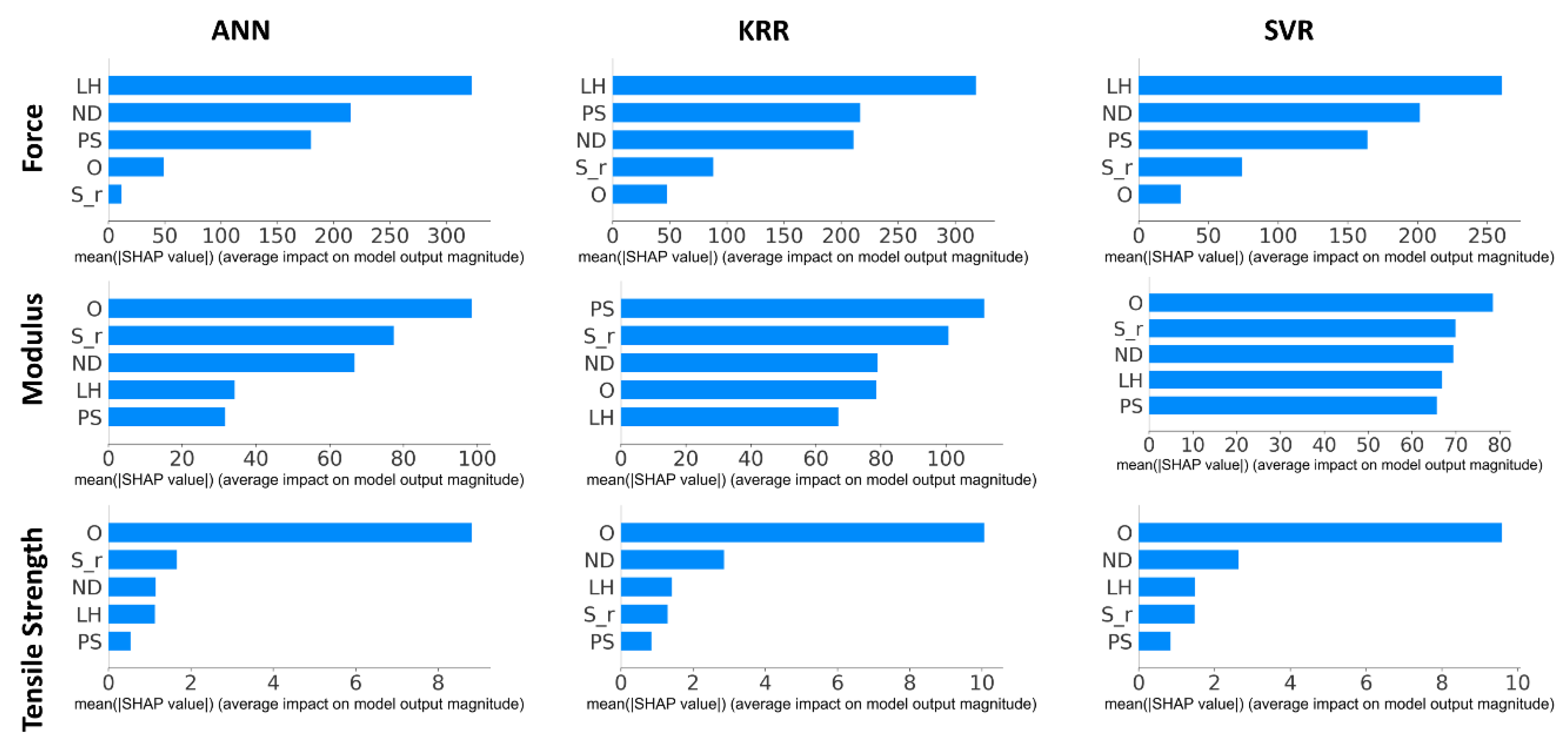
This work based on the material extrusion process not only establishes a multi-output algorithm encompassing both printer health detector—extrusion force—and the final part performance—tensile properties, which are highly related to the selection of various printing parameters, but also draws conclusions on the degree of influence wielded by each parameter on the prediction of these critical properties, which would be beneficial to elucidating the intricate relationships between inputs and outputs. Experimental work involved producing 476 tensile coupons, developed under various printing conditions, where the filament extrusion speed and filament extrusion force were measured in real-time using machines fitted with in-line sensors. These coupons were then tested up to tensile failure. The collective data of printing parameters, measured process indicators, and mechanical test results were used to train multi-output algorithms capable of predicting the tensile properties and extrusion force. To have a peek inside each prediction model, the Shapley value was studied and revealed the contributions of each input factor to the output prediction. In the end, the ML resources developed can potentially support the application of AM technology in the assessment of part structural integrity through simulation and also be integrated into a control loop that can pause or even correct a failing print if the expected filament force-speed pairing is trailing outside a tolerance zone stemming from ML predictions.

2. Methodology

2.1. Design of Experiments

The target values of the predictive ML system are the required average extrusion force F for the print, the tensile strength of the coupon σ_t, and the elastic modulus of the sample E. In order to capture a variety of printing conditions, the selected controlled variables varied in a three-level, full-factorial experimental layout, which can be seen in

Table 1. Controlled variables in the design of experiments.

Variable	Levels
Layer Height (hL) [mm]	0.1, 0.2, 0.4
Nozzle Diameter (DN) [mm]	0.3, 0.4, 0.8
Print Speed (Uxy) [mm/min]	1200, 2400, 3600

. Each printing condition was replicated twice to account for variability in the samples, and all combinations were reproduced using both a 0° and 90° orientation. Since the σ_t of a coupon cannot be measured for both load directions at the same time, given the destructive nature of the test, the orientation associated with each σ_t value was stored in a separate field, aptly named “orientation”.

The response surface method (RSM) is selected to make statistical predictions as it can quickly and effectively explain the relationships, linear or not, among several factors [18,19,20]. The linear regression is not complex enough to present the relationship between the inputs and each output based on the Pearson correlation matrix shown later. The quadratic term and two-faction interactive term are introduced to the regression system with a balance between fitting ability and model parsimony. Specifically, the prediction y from second-order polynomial response surface model is determined by the fitting of independent variables $x_i \mathrm{a}\mathrm{n}\mathrm{d} x_j$ from experimental data in the formula with model constants, linear, non-linear, and cross product coefficient ${\beta }_0$, ${\beta }_i$, ${\beta }_{ii}$, and ${\beta }_{ij}$, as shown in Equation (1). In this work, the coefficient of determination R² from RSM is used as a benchmark to compare against the several models of ML explored in this work, reflecting the necessity of using more complex algorithms in property predictions for FFF parts.

$$y={\beta }_{0 }+\sum _{i=1}^k{\beta }_{i }{x}_{i }+\sum _{i=1}^k{\beta }_{ii }{x}_i^2+ \sum _{i<j}^k{\beta }_{ij }{x}_{i }{x}_{j }+ \epsilon$$

(1)

2.2. Equipment and Methods

A set of 4 identically customized ME 3D printers (Minilab by FusedForm, Bogotá, Colombia) fitted with sensors capable of recording the force exerted by the filament upon the nozzle, discrete measurements of temperature, and changes in the extruded length over time were used to reproduce a variety of tensile coupons. A schematic of the printer setup can be seen in Figure 2. The data was collected using an Arduino board sampling at a frequency of 5 Hz, connected to MATLAB for visualization, processing, and logging. A Butterworth filter was applied to amplify the signal-to-noise ratio of the outputs of the system. The force sensor and encoder have an innate uncertainty of ±10 g and 600 pulses per revolution respectively. And the extruder motor has 200 pulses per revolution. A random set of printing conditions was reproduced on all printers to monitor printer-to-printer variability. More information pertaining to the construction of the printer and processing of the data can be found in the work of Mazzei Capote et al. [5]. Except for inline force measurement, the application of a pressure sensor at the heating block can also characterize rheological performance.

To minimize the impact of lurking variables, the filament was extruded in-house using the SABIC Cycolac MG94 ABS material, using an extrusion line that maintained the filament diameter within the target of 1.75 ± 0.05 mm using a vacuum-assisted water bath, a laser micrometer, and a conveyor belt in a control loop. Each filament was dried for a minimum of 3 h at 65 °C and kept in a dry box attached to the printer during manufacturing. Bed leveling was performed after 10 prints, or each time a change in material or nozzle was necessary. Nozzles were burned off in a furnace every time they were switched to minimize the influence of clogging.

Each print consisted of four rectangular tensile coupons of dimensions 25 mm by 100 mm by 3.2 mm, chosen to strike a balance between being relatively quick to print, having at least 50 mm of the gauge length, and fitting in the jaws of the tensile testing equipment. Each coupon was printed in a part-by-part manner (as opposed to having a single layer of print construct a slice of all coupons) to approximate real printing behavior as much as possible. Since a single experimental run yielded four coupons, post-processing was required to separate the force-data-speed pairings for each specimen. A pause was introduced between each part that would allow discerning when one specimen print was finished and the next started. A schematic of the process is shown in Figure 3.

Additionally, as an exploratory experiment, the geometric information of the filament was collected and paired with the rest of the information stemming from the in-line measurements of a handful of prints to assess if variations in the filament geometry resulted in notable changes in the required extrusion force. This data was attained through the use of a laser micrometer and a conveyor belt, pulling the material at a constant, known speed. The process yielded discrete measurements of the filament diameter and ovality as a function of filament length and time. A schematic of the process can be seen in Figure 4, where a symbolic diameter D changes over time t is shown. The locations of lasers are labeled as A, B, and C.

Tensile testing was performed using an Instron 5967 dual-column universal testing machine fitted with a 30 kN load cell. All data acquisition was handled through the accompanying Instron Bluehill 3 software. A movement speed of 5 mm/min was used to deform the 50 mm gage section of the specimens, with all deformations being logged using an extensometer. To protect the samples from the excessive gripping force, emery cloth tabs were used [21]. This setup can be seen in Figure 5. The final step of the process involved matching the printing data to its corresponding mechanical test results and assembling everything in a single database. This was conducted using Python code that would search the directory of the raw data and construct a .csv file including all the pertaining information of an experimental run in a row. This step is necessary for the ML code to quickly read and understand the information that it is attempting to model.

An additional metric that can aid in identifying underlying systematic issues or relationships between the print and its mechanical properties is comparing the theoretical filament speed S_t against its experimentally measured counterpart S_m. The theoretical filament speed can be calculated using a simple volumetric balance. The volume of an extruded bead can be approximated as $h_L·D_N·l$, where l represents the bead length. Given that mass must be conserved, this implies that the volume of the bead $V_{out}$ must be equal to the volume supplied by the incoming filament $V_{in},$ resulting in Equation (2), where D_f and L represent the filament diameter and length supplied to extrude the bead, respectively:

$$V_{out}=h_L·D_N·l=V_{in}=\frac{\pi ·D_f^2·L}{4}$$

(2)

Manipulating Equation (3) to solve for L results in:

$$L=\frac{h_L·D_N·l·4}{\pi ·D_f^2}$$

(3)

Now, one can use the expected time to print a bead of dimensions $l$ to solve for the expected filament speed S_t.

$$t=\frac{l}{U_{xy}}$$

(4)

Finally, converting units and combining Equations (3) and (4) yields the theoretical filament speed, S_t.

$$S_t=\frac{4·h_L·D_N·U_{xy}}{\pi ·D^2}$$

(5)

This information can be used to verify if the printer is under-extruding by comparing the theoretical filament speed with the measured value. In ideal conditions, the real-to-expected ratio $\frac{S_{m }}{S_{t }}$ approaches 1. Any deviation indicates that less or more material was deployed during printing, indicating a problem during the print or toolpath that led to under- or over-extrusion.

2.3. Proposed Supervised Machine Learning Algorithms for Regression

2.3.1. Artificial Neural Network

A neural network (NN) algorithm is effectively a facsimile of how biological neurons establish connections and communicate with each other. In summary, the inputs of the problem are fed to a layer of nodes, or “neurons”. Each node has a variety of connections to other neurons and an associated weight and activation threshold, which, if surpassed, triggers information transfer to its connections in subsequent layers. Finally, the information reaches the network stratus that estimates the outcome of whatever phenomena the model is trying to characterize, traditionally named the output layer [10,22,23]. The weights and activation thresholds of each node are iteratively tuned as the NN architecture is exposed to a training data set while also being compared to a separate set of data points used for validation. Once the accuracy of the model reaches its desired value, the underlying communication between the neurons is capable of making predictions based on what the input layer is perceiving [9]. This type of architecture tends to be reserved for computationally complex tasks, such as text recognition or image processing.

The capability of NNs to model complex behaviors is rooted in the mathematical operations that happen behind the scenes. Each neuron behaves effectively as its own mini-linear regression model, represented in Equation (6). Here X_i and W_i represent one of the node’s m inputs and its associated weight, respectively.

$${\displaystyle \sum _{i=1}^m}{W}_i{X}_i+\mathrm{b}\mathrm{i}\mathrm{a}\mathrm{s}=z$$

(6)

The weighted sum of the inputs can then be used as is or passed through an activation function. This signals the generation of an output that can then be used at face value or transmitted to subsequent nodes if a threshold is surpassed.

Concatenating nodes in a forward fashion creates the concept of levels or layers in a network. When all neurons in a layer are fully connected to the nodes in the previous level, this is typically called a dense layer. Arranging more than one dense layer in a series results in a NN [10,23].

The weights of each neuron are iteratively tuned in a process that involves penalizing the model using a loss function that compares the predictions of the model with true output values using example data. This process is effectively an optimization task where the goal is to minimize the loss function. A schematic of the process can be seen in Figure 6, using a two-layer network architecture as an example.

2.3.2. Pipeline

In addition to the artificial neural network, other regressors were also explored to create multiple output models. This was achieved by combining a pipeline tool to organize a list of feature scaling and regression and the GridSearchCV method from scikit-learn to optimize hyperparameters by cross-validation based on a parameter grid.

The pipeline is composed of scaling and regression, as shown in Figure 7. Scaling refers to a linear transformation with the purpose of avoiding feature prioritization. The most common scaler is called the “Standard Scaler”, which transforms features by subtracting the mean value and dividing by the standard deviation. Another common scaler, called the “Robust Scaler”, subtracts the median value over the interquartile range. Both scalers are selected as candidates in the pipeline under the scaler section.

There are three commonly used regressors that were applied to our pipeline directly due to their capability of handling multi-output problems. These were K-Nearest Neighbors (KNN), Decision Tree Regressor (DTR), and Kernel Ridge Regression (KRR). The regressor with its specific hyperparameter value that has the lowest Root Mean Square Error (RMSE) based on the training data was considered the best result out of all the options listed in the pipeline, which was kept for the final decision. In detail, the K-Nearest Neighbors (KNN) Regressor is a neighbors-based regression algorithm based on local interpolation of the data points with a predefined number of nearest neighbors (named k) training data. The hyperparameter k requires tuning using techniques such as grid search cross-validation, covered in a section below. The Decision Tree Regressor (DTR) solves the regression problem by using a set of if-then-else decision rules. The higher the max depth of the tree, the more complex the fitting, with the risk of overfitting. Kernel Ridge Regressor (KRR) is a combination of ridge regression and the kernel trick. The purpose of Ridge Regression is to minimize the summation of squared residuals between real outputs and predictions, plus a penalty parameter λ multiplied by the slope β squared [25]. This type of model also requires tools like cross-validation for hyperparameter tuning. Ridge Regression on its own is limited to linear relationships. If this condition is not met, it is necessary to use the kernel trick to allow compatibility with this algorithm. Kernel trick projects data by a mapping function, such as the radial basis function (RBF), used in this study. This mapping function can be seen as a weighted K-Nearest Neighbor Algorithm with an infinite number of dimensions [26]. Gamma is a hyperparameter in RBF that scales the squared distance between each pair of input data points, which implies fine-tuning through cross-validation.

2.3.3. Support Vector Regressor

Support Vector Regressor (SVR) is another popular regressor used in supervised ML. The fundamental idea of SVR is similar to that of Support Vector Machine (SVM) [27], but SVR focuses on fitting a hyperplane that includes the maximum number of training observations within a margin. For a detailed explanation of how the algorithm works and the hyperplane optimization, the reader is invited to read the work from Xu et al. [28]. A kernel trick is also required to be a bridge between linear and non-linear phenomena for conversion purposes. Another adjustment to SVR that allows it to be applicable to this multi-output case is adding MultiOutputRegressor on top of it; otherwise, SVR can only support one output each time [29].

2.3.4. Parameter Optimization Based on GridSearchCV

GridSearchCV (GSCV) is a modulus under sklearn for hyperparameter optimization with cross-validation (CV). CV is an evaluation method that involves training the algorithms multiple times with different partial training data and evaluating them with a complementary subset of training data [30]. The main sections include the estimator and the corresponding parameter grid. The combination of cross-validation and grid search is an efficient way of determining the best hyperparameters within the parameter grid. And the pipelines can be used as estimators. The workflow is shown in Figure 8. The scaler and regressor candidates are listed in the pipeline, which is fed into the grid search system for determining the best combination of the provided parameter options with training data. The best model will be applied to testing data for a final evaluation.

2.3.5. Shapley Values

While ML algorithms are powerful, highly adaptable predictive models, the contributions of each input are usually hidden behind a veil of complexity that makes it almost impossible for the user to comprehend what is happening behind the scenes. Luckily, recent developments in the interpretability of models allow a peek inside the inner machinations of a NN, normally considered a “black box” model. Of particular interest is the application of Shapley values to aid in the understanding of how a trained ML model is affected by each of its inputs.

A Shapley value is a concept that stems from game theory. To paraphrase and oversimplify the formal definition, if a coalition $C$ collaborates to produce a value V, the Shapley value is simply how much each member of the coalition contributed to its final output [31,32]. This meaning can be extended to how much each input of a model is contributing to its output, according to the focus of this work. The formal mathematical definition is computationally expensive and escapes the scope of this work, but a numerical approximation using Monte-Carlo sampling, proposed by Strumbelj et al. [33], states that, for any model f capable of making a prediction using the vector x with M features as an input, the Shapely value ${\widehat{\varphi }}_J$ for that particular input can be approximated as follows:

$$\frac{1}{M}{\displaystyle \sum _{m=1}^M}\left(\widehat{f}\left(x_{+j}^m\right)-\widehat{f}\left(x_{-j}^m\right)\right)={\widehat{\varphi }}_J$$

(7)

where $\widehat{f}\left(x_{+j}^m\right)$ and $\widehat{f}\left(x_{-j}^m\right)$ represent predictions made by the model using two synthetic datapoints, constructed using a random entry from the database, called z. The former term is the instance of interest, but all values in the order after feature $j$ are replaced by feature values from the sample z. Similarly, the latter term, $\widehat{f}\left(x_{-j}^m\right)$ is constructed in the same manner as $\widehat{f}\left(x_{+j}^m\right)$, but it also replaces feature j by its counterpart from datapoint $z$ [32].

To facilitate its applicability to ML, Lundberg and Lee created the SHAP (Shapley Additive Explanations) method to explain individual predictions. The SHAP method effectively models “any explanation of a model’s prediction as a model itself, termed an explanation model [34]. Finally, for the purposes of SHAP, the explanation model of choice has each effect ${\varphi }_i$ attributed to a feature, and the sum of the effects of all feature attributions approximates the outputs of the original model f. This explanation model is represented by the equation below:

$$g\left(z^{\prime }\right)={\varphi }_0+{\displaystyle \sum _{m=1}^M}{\varphi }_i{z}_i^{\prime }$$

(8)

Using Equations (7) and (8), one can use Shapley values to identify the importance of features in a respective model. This allows the user to make decisions pertaining to the architecture of the model as well as appreciate the impact a particular input can have on the output of the model, something that would be difficult to do without this resource. These mathematical principles are built into the SHAP Python library out of the box [34].

3. Results and Analysis

3.1. Experimental Results

3.1.1. Effect of Variations in Filament Diameter upon Extrusion Measurements

The effect of fluctuations in the filament geometry on the required extrusion force is unknown but is expected to be proportional given the current filament extrusion models. As an exploratory experiment, the data stemming from the measurements of the laser micrometer during filament production were matched to the corresponding data readings resulting from the printer sensors. The condition chosen to test this experiment was $h_L=0.2 \mathrm{mm}$, $D_N=0.4 \mathrm{mm}$, $U_{xy}=2400 \mathrm{mm}/\min$. Matching the filament diameter and ovality measurements to the corresponding speed and force readings from the sensors resulted in inconclusive results. This can be seen in Figure 9, where the force remains nearly constant despite the variations in filament diameter and ovality.

Pairing the geometric information of the filament to its corresponding print data proved to be an extremely time-consuming task, given that both sets of information came from different devices and that in order to obtain proper matching, the starting point of the print had to be accurately pinpointed as length zero. The inconclusive nature of these results and the additional time required to further explore this phenomenon lend themselves well to future work with a device that measures the filament geometry directly within the printer to facilitate exploring trends over more printing conditions.

3.1.2. Printer Sensor Data Analysis

Generally speaking, the average measured filament speed was very consistent within a particular print condition. The standard deviation for filament print speed data varies between $6.6·{10}^{-4}$ and 1.8 mm/s. In contrast, the measured print force varied drastically between experimental runs and even within the same print. As an example, four print coupons produced in a single print using $h_L=0.2\mathrm{m}\mathrm{m},D_N=0.4\mathrm{m}\mathrm{m},U_{xy}=2400\mathrm{m}\mathrm{m}/\mathrm{m}\mathrm{i}\mathrm{n}$ had average forces of 792.66, 611.52, 516.86, and 554.91 g, respectively. The standard deviation of the measured print force ranged between 16 and 475 g, with higher variability observed in prints involving the smallest nozzle diameter combined with the largest layer height. The conditions selected to test experimental reproducibility between printers showed no higher variability than fluctuations of measured force and filament speed within the same printer, with the highest discrepancy between printers in the range of 100 g and $1·{10}^{-3} \mathrm{mm}/\mathrm{s},$ respectively.

For most conditions, the measured filament speed approximated the theoretical value fairly closely, with most specimens achieving a real-to-expected speed ratio $S_r$ between 0.95–0.97. However, a couple of generalizations can be made for certain combinations of experimental values that had ratios below 0.9. These involved the fastest U_xy combined with a h_L that was larger than the D_N, namely, a 0.3 mm N_D paired with a 0.4 mm h_L. It is believed that this is caused by filament force requirements that go beyond the capabilities of the machine, resulting in slippage at the drive wheel of the system. This effect was present in more conditions in the 90° orientation; in particular, conditions that involved the 3600 mm/min gantry speed. This is theorized to be caused by a shorter travel distance between contiguous beads, implying that the acceleration of the system was not sufficient to attain the desired filament speed before the tool pass required a change in direction.

3.1.3. Tensile Testing Results

Tensile results showed good agreement between replicates. The exceptions came mostly in the conditions that involved the largest h_L combined with the lowest D_N; in particular, those printed using the two fastest printer speed U_xy. One can conclude that this response is rooted in printing defects introduced due to the difficulty of the printhead sustaining the necessary pressure during the manufacturing of the coupons under these conditions. The standard deviation ranged from as low as 86 and 0.19 MPa to as high as 931 and 7.56 MPa for E and the σ_t, respectively.

3.2. Statistical Analysis and Results

The analysis of the data was performed in two ways. First, using the entire data set to develop a Pearson correlation matrix; and second, analyzing as a full-factorial experimental design, separating the data set into two parts: one for each printing orientation.

The Pearson correlation matrix allows for discerning whether variables and a response may possess a linear correlation with each other, with a coefficient of 1 (or −1) indicating perfect linear correlation. It should be noted that a low Pearson index does not mean no correlation; it simply implies that the relationship may not be linear in nature [23]. The resulting matrix can be seen in Figure 10. Here it can be seen that out of all responses of interest, except the relation between σ_t and O, F shows a high likelihood of linear correlation with the h_L, D_N, U_xy, and S_r.

The factorial experimental analysis of variance (ANOVA) yields results relating to how the input variables can have direct or interacting effects on the measured response. Starting with the 0° orientation, the ANOVA test determined that using a $95\mathrm{\%}$ confidence interval, the F is directly affected by the main effects of the selected control variables, as well as its two- and three-way interaction effects. A similar conclusion can be drawn for the σ_t. Interestingly, only the Nozzle Diameter and the Print Speed have tangible main and interaction effects on the Elastic Modulus. Results can be seen in

Table 2. Summary ANOVA table of 0° experiments.

	F		E		σt
Effect	f	p-Value	f	p-Value	f	p-Value
hL	349.41	*	2.17	0.117	382.56	*
DN	361.45	*	11.3	*	3.44	0.034
Uxy	213.43	*	9.37	*	9.17	*
hL ∗ DN	15.05	*	1.17	0.326	16.10	*
hL ∗ Uxy	44.5	*	3.21	0.014	30.16	*
DN ∗ Uxy	4.77	0.001	1.22	0.304	35.95	*
hL ∗ DN ∗ Uxy	3.97	*	0.67	0.714	53.64	*

, where * denotes a p-value lower than 0.001.

Applying the same type of analysis to the 90° population yields similar results. Here, at a $95\mathrm{\%}$ confidence interval, U_xy, h_L ∗ D_N, and h_L ∗ U_xy do not play a significant role in the response of E, while the h_L does not affect σ_T. All other main and interaction effects are considered significant at the selected $\alpha =0.05$ value. The results of the ANOVA test can be seen in

Table 3. Summary ANOVA table of 90° experiments.

	F		E		σt
Effect	f	p-Value	f	p-Value	f	p-Value
hL	416.87	*	3.37	0.039	0.37	0.693
DN	122.68	*	25.24	*	234.96	*
Uxy	166.16	*	2.84	0.064	41.39	*
hL ∗ DN	13.09	*	0.62	0.649	25.51	*
hL ∗ Uxy	66.31	*	2.33	0.063	21.86	*
DN ∗ Uxy	22.28	*	13.77	*	14.30	*
hL ∗ DN ∗ Uxy	41.20	*	5.90	*	16.71	*

, where * denotes a p-value lower than 0.001.

To further clarify the interconnectivity between input factors and response predictions, the RSM was implemented to generate empirical models with a $95\mathrm{\%}$ confidence interval. As orientation is a categorical factor, the model equations do not involve such a factor but were divided into two branches by orientation, which are shown in

Table 4. Summary of the regression models from the Response Surface Methodology.

Response Variable	Model Equation
	0°	90°
F [g]	$6979-6302 h_L-7839 D_N-1.347 U_{xy}-5288 S_r+2568 h_L\ast h_L+8385 D_N \ast D_N+0.000031 U_{xy}\ast U_{xy}+1649 S_r\ast S_r-1780 h_L\ast D_N+1.664 h_L\ast U_{xy}+4560 h_L\ast S_r+0.0923 D_N\ast U_{xy}-2464 D_N\ast S_r+1.073 U_{xy}\ast S_r$	$5622-4721 h_L-8157 D_N-1.241 U_{xy}-4143 S_r+2568 h_L\ast h_L+8385 D_N\ast D_N+0.000031 U_{xy}\ast U_{xy}+1649 S_r\ast S_r-1780 h_L\ast D_N+1.664 h_L\ast U_{xy}+4560 h_L\ast S_r+0.0923 D_N\ast U_{xy}-2464 D_N\ast S_r+1.073 U_{xy}\ast S_r$
E [MPa]	$11425-\mathrm{10,724} h_L-781 D_N-2.153 U_{xy}-\mathrm{10,552} S_r-2921 h_L\ast h_L-436 D_N\ast D_N+0.000122 U_{xy}\ast U_{xy}+2666 S_r\ast S_r+2156 h_L\ast D_N+0.256 h_L\ast U_{xy}+\mathrm{10,731} h_L\ast S_r+0.197 D_N\ast U_{xy}-86 D_N\ast S_r+1.424 U_{xy}\ast S_r$	$9441-9988 h_L-833 D_N-1.954 U_{xy}-9207 S_r-2921 h_L\ast h_L-436 D_N\ast D_N+0.000122 U_{xy}\ast U_{xy}+2666 S_r\ast S_r+2156 h_L\ast D_N+0.256 h_L\ast U_{xy}+\mathrm{10,731} h_L\ast S_r+0.197 D_N\ast U_{xy}-86 D_N\ast S_r+1.424 U_{xy}\ast S_r$
σt [MPa]	$130.1-260.0 h_L-57.6 D_N-0.01283 U_{xy}-97.8 S_r+58.7 h_L\ast h_L-7.52 D_N\ast D_N+0.00 U_{xy}\ast U_{xy}+18.5 S_r\ast S_r+48.24 h_L\ast D_N+0.01092 h_L\ast U_{xy}+171.4 h_L\ast S_r+0.00483 D_N\ast U_{xy}+51.2 D_N\ast S_r+0.00951 U_{xy}\ast S_r$	$114.5-219.2 h_L-82.0 D_N-0.01373 U_{xy}-95.2 S_r+58.7 h_L\ast h_L-7.52 D_N\ast D_N+0.00 U_{xy}\ast U_{xy}+18.5 S_r\ast S_r+48.24 h_L\ast D_N+0.01092 h_L\ast U_{xy}+171.4 h_L\ast S_r+0.00483 D_N\ast U_{xy}+51.2 D_N\ast S_r+0.00951 U_{xy}\ast S_r$

. In addition to being able to more intuitively see the degree of impact of each variable or variable group on the final prediction result, more attention is paid to the accuracy of the prediction result under this method. In

Table 5. Summary of the proportion of variance from Response Surface Methodology.

Response Variable	R2	Adjusted R2	Predicted R2
F [g]	0.8410	0.8344	0.8227
E [MPa]	0.2949	0.2655	0.2291
σt [MPa]	0.9331	0.9303	0.9255

, the overall summary of accuracy for each output variable is shown, which considers both orientations together. R² measures the variation in a regression model, while adjusted R² is the proportion of variance, which eliminates the interference of the number of predictors and dataset size in prediction. In order to further simulate the performance of the model in the prediction, the predicted R² is to use the number set ignored by the fitting process for the calculation of the proportion of variance. Therefore, whether the values of the proportion of variance are close to 1 or the values of the various R² are close to each other is equally important when judging the results of the regression model. In Table 5, the values for three R² are not far away from each other when compared within each response variable, which means overfitting is not an issue. However, the values of R² have a significant difference between 1, especially for modulus prediction. There are two possible reasons: one is that the complexity of the models is not high enough to capture the data trend. The other one is that the captured predictors are not comprehensive enough for the prediction of the response variable. Therefore, the various machine learning algorithms are reported below to give the answer.

3.3. Machine Learning Results

In order to more intuitively show the performance of different trained models in predicting output, results from different models will be compared horizontally. Specifically, the content of the first subtitle mainly shows the best hyperparameters and architectures of the trained model. The second part revealed the accuracy of each model based on the test data and the ranking of the influence of each input on the output during the prediction process. The last part is the comparison of the implementation experiments accuracy of each model.

3.3.1. Optimal Model for Each Architecture

The NNs described in this section were developed using the TensorFlow platform for Python, using the Keras API. The algorithm was trained using a stratified, random split approach that maintained the ratio of 0° and 90° samples to avoid the accidental introduction of biases to the NN. This ratio was estimated to be 51:49$,$ respectively. The split was set to the typical 80-20 split, where 80% of the data goes to train the model and the remaining 20% is stored separately and used to validate the system and check for overfitting or underfitting. In order to facilitate the convergence of the algorithm to its optimal configuration, the data were normalized by using Equation (9) prior to being used by the model. In this computation, X is a feature, $\mu$ is the mean of the feature values, and σ is the standard deviation. This ensures all entries in the dataset have a comparable scale.

$$X^{\prime }=\frac{X-\mu }{\sigma }$$

(9)

Except for the output neurons, all nodes had the activation function set to the Rectified Linear Unit (ReLU) function. This activation function is generally considered to be superior to most common alternatives and is relatively easy to compute. Its formula simply outputs the positive part of the argument. Should the input be negative, the output is zero. The chosen loss function for the model was the Mean Square Error (MSE) function, represented in Equation (10), where $Y_i-{\widehat{Y}}_i$ represents the difference between model prediction and real value and n represents the number of data points used to compare model and reality.

$$MSE=\frac{1}{n}{\displaystyle \sum _{i=1}^n}{\left(Y_i-{\widehat{Y}}_i\right)}^2$$

(10)

The optimizer function chosen for this study was the “Adam” proposed by Kingma and Ba [35]. This optimizer offers a mixture of the advantages offered by Stochastic Gradient Descent (SGD) and traditional Gradient Descent (GD), with the caveat of adding additional parameters to the model. This approach avoids the erratic behavior of SGD as it approaches the minimum of the loss function while ensuring that the model converges as rapidly as possible.

The network architecture involved a single input layer and three branches. Each branch computes the output of the expected F, E, and σ_t. Each branch contains two dense layers, with a “dropout” layer in between. This process randomly removes a number of neurons from the preceding layer temporarily with each iteration of the training process, ranging from 0% to 100% of the neurons. This has the effect of ensuring the network adapts by establishing connections that are truly meaningful between nodes, which tends to prevent overfitting. The chosen rate of dropout for all dropout layers was 0.5, meaning that each epoch, 50% of the neurons was temporarily removed from the model. A schematic representation of the model generated through TensorFlow can be seen in Figure 11. The inputs of the network were the 4 controlled variables and the ratio of the measured filament velocity against the expected filament velocity derived from a volumetric balance, resulting in 5 inputs.

Custom code was developed using the keras tuner utility to iterate through multiple variations of this architecture to achieve the highest performance possible during training in a systematic manner. This code would train different versions of the model using different numbers of neurons per layer and varying the learning rate of the optimizer function. A list of the model hyperparameters can be found in

Table 6. Neural network hyperparameters of note.

Hyperparameter	Value
Learning Rate	[1 × 10−4, 1 × 10−2]
Number of Neurons per Layer	[32, 72]
Batch Size	20
Max. Number of Epochs	30
Early Stopping Patience	5

. The optimal model architecture per hyperparameter tuning process uses 64 neurons per layer and a learning rate of 0.00972.

To compare the performance between different ML algorithms, the R² was considered an indicator. The same training and testing data sets are used to ensure the credibility of the comparison. For the other ML algorithms implemented through the pipeline, the chosen parameter options are listed in

Table 7. Selected values of hyperparameters in the pipeline for cross-validation.

Regressor	Parameter	Selected Values
KNN	Number of neighbors	[5, 11]
DTR	Max depth	[2, 4]
KRR	Penalty parameter λ	[1 × 10−3, 1]
	rbf kernel parameter γ	[1 × 10−2, 1 × 102]

. With the comparison between all regressor candidates with a variety of hyperparameters in the pipeline, the optimal model under this architecture is the combination of the Kernel Ridge Regressor (λ = 0.01, γ = 0.1) and the standard scaler.

SVR has two hyperparameters that must be optimized by cross-validation. One is regularization parameter C for controlling the balance between good fitting with training datasets and maximizing the function’s margin; the other is γ in the RBF kernel function for controlling the radius of the influence of samples selected by the model as support vectors. The selected values for each parameter are listed in

Table 8. Selected values of hyperparameters in SVR for cross-validation.

Regressor	Parameter	Selected Values
SVR	Regularization parameter C	0.1, 1, 100, 1000
	RBF kernel parameter γ	0.01, 0.1, 1, 10, 100

below. With cross-validation, the best hyperparameter combination was determined (C = 1000, γ = 0.1).

3.3.2. Testing Results Comparison

Using the optimal architecture to train the NN model yielded the results shown in Figure 12. These plots show that the model converges to a minimum, and there is no evidence of overfitting. Here, the blue line shows the change in the RMSE during the training step, while the green line tracks the validation procedure.

Comparing the other two ML approaches and RSM, it can be seen in

Table 9. R² comparison between different ML algorithms and RSM.

Model	F	E	σt
ANN	0.807	0.184	0.8545
KRR	0.907	0.163	0.93
SVR	0.909	0.346	0.974
RSM	0.841	0.295	0.933

that the SVR algorithm has the highest R² for F, E, and σ_t outputs. From here, it can be seen that increasing the nonlinearity of the model does not necessarily lead to better prediction accuracy. Compared with ANN, SVM has an advantage in predicting samples with limited data by using quadratic optimization and penalizing parameters to avoid falling into local minimums and overfitting [36]. Performance was relatively poor in terms of E prediction for all tested algorithms. This is visualized in Figure 13, where the true value of a response is plotted against the prediction of the model. A model that perfectly captures the behavior of the system is represented by a line of slope 1. Note that for all models, the corresponding graph of the predicted versus true value of E shows large deviations from the ideal behavior slope. The data for E showed the largest variability within replicates out of all of the measured outputs, which may explain why the algorithms have difficulty converging to a solution close to the “true” value.

Exploring the SHAP results of the models allows one to draw conclusions regarding how each ML solution is making predictions and potentially inform how to fine-tune a second iteration of the architecture of the best-performing system. This resource can be interpreted as how much each feature of the model contributes to the final predicted value on average. For instance, using the predicted extrusion force as an example, changes in the layer height of a print will generally result in a change of roughly 300 g in the expected print force on all models. By contrast, the filament speed ratio results in a change between 10 g and 100 g, depending on which ML solution is being examined. Fine-tuning the model is not as simple as removing the features with the lowest Shapley values. As indicated by the statistical analysis of the data set, the interacting effects of all controlled variables were rarely negligible. Additionally, most of the experiments performed to acquire the data yielded filament speeds that closely matched the theoretical filament speed; thus, the small contribution of the filament speed ratio could be attributed to a near-uniform population.

Starting with the ANN construction, for force output F, the greatest absolute average Shapley value was attributed to the h_L. Next, both U_xy and D_N had Shapley value attributions of roughly half of that of h_L. Finally, the print orientation O and the filament speed ratio S_r had the lowest values, with O having a Shapley value of roughly 1/6 of the attribution of h_L, while S_r had an average impact of around 1/30. These results are better appreciated in the upper left corner of Figure 14. A similar analysis can be made using the Shapley values of the other outputs from various models.

SHAP results from KRR and SVR are shown on the second and third columns separately in Figure 14. The weight of each input variable for F and σ_t prediction from KRR and SVR is slightly different from the conclusion driven by ANN, but the layer height always has the highest contribution to F prediction and the orientation has the most significant influence on the prediction on σ_t, which could lead to similar RMSE values for F and σ_t predictions. However, the weights show a significant difference in E predictions between KRR and the other two. Instead of considering orientation as the most important factor in modulus prediction, the weights from KRR have a more even distribution than ANN prediction, and printing speed is at the top of the rank, which could be the reason for the hardness of E prediction. Every input has a relatively even contribution to the output, which makes the algorithm hard to converge with such many flexibilities. Orientation was only the most important contributor to predictions of σ_t, which is theoretically supported since orientation has been shown through other studies to have a significant impact on the modulus of printed coupons [37]. All models place the factors that affect volumetric throughput ($D_N, h_L, U_{xy}$) as the most important when dealing with predictions of extrusion force, which agrees with theoretical melting models based on transport phenomena [4,38,39].

While the models proved acceptable at predicting the expected F and σ_t of the part, the capabilities to predict E should be improved. Future work could explore additional architectures using the findings from this work or increase the data size by performing additional experiments introducing more speed ratios under different printing conditions, such as over-extrusion and under-extrusion. They can be used to train models with the ability to detect bad printing conditions.

3.3.3. Implementation Results Comparison

New printing conditions, not explicitly tested during the training and validation steps described before, were used to produce coupons to further validate the best models. The only information supplied to the ML solution is the input values shown below in

Table 10. Printing parameters for model verification.

Variable	Levels
Layer Height (hL) [mm]	0.2
Nozzle Diameter (DN) [mm]	0.5
Print Speed (Uxy) [mm/min]	2400

. The dimensions of the sample were once again 25 mm by 100 mm by 3.2 mm.

Following the same procedure as before, each print consisted of 4 coupons, and each print was repeated 2 times. The printing parameters and experimental data of 8 samples are shown in

Table 11. Experimental data for verification samples.

Sample	O [°]	hL [mm]	DN [mm]	Uxy [mm/min]	Sr	F [g]	E [MPa]	σt [MPa]
1	0	0.2	0.5	2400	0.959	517.398	2417.93	37.49
2	0	0.2	0.5	2400	0.961	499.294	2354.26	37.53
3	0	0.2	0.5	2400	0.962	507.528	2038.77	36.5
4	0	0.2	0.5	2400	0.961	522.450	2338.16	35.73
5	0	0.2	0.5	2400	0.967	582.357	2053.77	37.03
6	0	0.2	0.5	2400	0.963	579.558	2083.33	37.03
7	0	0.2	0.5	2400	0.965	597.970	2179.39	35.81
8	0	0.2	0.5	2400	0.9636	603.746	2022.44	35.7

. To be able to observe the data distribution more clearly for each output category, the box and whisker plots were made separately for each category. It can be seen in Figure 15 that the variation of the speed ratio of various samples is relatively low, but the output values, especially F and E, have a certain degree of variation on each replicate. Consequently, all eight speed ratios from different samples are inputs in three models. The relative error between prediction and experimental values is calculated for the model’s performance evaluation.

Each machine learning algorithm has three outputs, which are compared with experimental data to capture relative error based on Equation (11). The absolute value of the difference between the prediction ($v_A$) and the experiment result ($v_E$) is the absolute error. Relative error is the ratio between absolute error and the experiment result, which can remove the influence from the value of the experiment result itself.

$$\delta =\left|\frac{v_A-v_E}{v_E}\right|\cdot 100\%$$

(11)

The relative errors of three outputs from three models are shown in Figure 16. For the printing F and σ_t predictions, SVR has relatively low relative errors, which are in the range of 5% to 10%. However, the E prediction by SVR has a larger range of relative error compared to the other two regressors. The samples #3, 5, 6, and 8 have high errors based on the trends of all three algorithms, which have a good match with the experimental results of the samples that have relatively low E, as shown in Table 9 above. As all input values of 8 samples are close to each other, the significant differences between outputs would contribute to prediction errors, especially in the scenario where the value range of the data is at a high level, which is between 2022.44 MPa and 2417.93 MPa. In this case, testing more samples for each condition could be a good way to eliminate the experimental bias in the future. Overall, the SVM has the best performance on the prediction of mechanical properties and printing force. This could be attributed to its punishment and margin-fitting regimes.

4. Future Directions

4.1. Expanding Model Applicability

The predictive tool centered on ABS material holds promise for further refinement and expansion, with a specific focus on broadening its applicability to encompass a wider range of materials. This potential evolution is founded upon the demonstrated feasibility of the workflow elucidated in this case study.

To elaborate, in addition to incorporating printing parameters, augmenting the input parameters to include material properties during processing is warranted. Parameters such as shear viscosity, density, heat capacity, thermal conductivity, glass transition temperature, or melting temperature have been highlighted in Osswald’s study as factors bearing significant relevance to heat transfer and the melting processes occurring within the nozzle [4].

Another interesting avenue to explore is the integration of polymer blends into s predictive models. The addition of compatibilizers, in particular, presents a noteworthy factor that can exert varying effects on the strength and toughness of printed coupons. While compatibilizers enhance adhesion between phase domains, they concurrently diminish the self-strengthening capacity during the polymer bead deposition process with a stretching-induced effect [40].

4.2. Prediction of Failure Envelope

As the model is capable of predicting the σ_t in the 0° and 90° orientations, it lends itself well to generate a very conservative version of the Stress-Stress Interaction Criterion (SSIC). Assuming that the failure at shear is approximately the failure at tension at 90°, that the failure stresses in compression are equal to their corresponding failure in tension, and that all stress interactions are 0, one could generate a SSIC failure envelope for a part as soon as it is finished printing. As an example, the failure envelope shown in Figure 17 and Figure 18 was developed for printing conditions ${\mathrm{h}}_{\mathrm{L}}=0.1\mathrm{m}\mathrm{m},{\mathrm{D}}_{\mathrm{N}}=0.3\mathrm{m}\mathrm{m},{\mathrm{U}}_{\mathrm{x}\mathrm{y}}=1200\mathrm{m}\mathrm{m}/\mathrm{m}\mathrm{i}\mathrm{n},{\mathrm{S}}_{\mathrm{r}}=0.96$. This could prove particularly useful for the automotive or aerospace industries, as all attempts known to the author to predict failure in AM through failure criteria are locked to a fixed set of printing conditions.

4.3. Detection of Print Defects or Printer Issues

As the model is capable of predicting the average print force required to extrude a polymer bead under a certain combination of the controlled variables, one could develop a system capable of alerting the user to stop the print or even perhaps self-correct the issue if the measured print force deviates wildly from the expected output. As anecdotal evidence that this is viable, the author experienced this first-hand during the experiments that measured the inter-printer variability. While performing a control print on the four printers, the force detected by one of the sensors was uncharacteristically high, differing from its other three counterparts by thousands of grams as opposed to the usual hundreds. After servicing the printer, the root of the issue was determined to be a degraded Teflon tubing within the heated chamber of the print head that greatly restricted the movement of the filament.

5. Conclusions

This work was able to create various ML solutions capable of predicting the expected extrusion force, Young’s modulus, and tensile strength of FFF parts produced using a specialized printer with sensors capable of measuring the filament extrusion speed and force. By comparisons on R² from testing data and on relative errors from verification data, the model trained by SVR has the best performance on the prediction of F and σ_t. With Shapley values and traditional statistical analysis, it was shown that most of the inputs and their corresponding interaction effects have a significant impact on the predictions from the model. The relatively weak predictive capabilities of E could be potentially improved by more supplemental data.

The predictions that stem from this resource can prove useful to engineers designing functional parts for AM, as the ML algorithms can predict arguably the two most critical mechanical properties necessary to estimate a failure surface. This work additionally extends the invitation for future work to be focused on a smart system that makes use of the sensors within the printer and the expected predicted extrusion force to detect print defects and either stop the print or autocorrect the issue. Expanding the utility of this prediction tool to encompass a variety of materials is also a feasible endeavor. Finally, the results presented here and the models developed have the potential to aid in the explanation of the underlying physics of how the FFF process tends to produce parts that are anisotropic. As such, there is ample room for further refinement and advancement of this prediction tool.

References

1. Tammaro, D. Rheological Characterization of Complex Fluids through a Table-Top 3D Printer. Rheol. Acta 2022, 61, 761–772. [Google Scholar] [CrossRef]
2. Coogan, T.J.; Kazmer, D.O. Modeling of Interlayer Contact and Contact Pressure during Fused Filament Fabrication. J. Rheol. 2019, 63, 655–672. [Google Scholar] [CrossRef]
3. Anderegg, D.A.; Bryant, H.A.; Ruffin, D.C.; Skrip, S.M.; Fallon, J.J.; Gilmer, E.L.; Bortner, M.J. In-Situ Monitoring of Polymer Flow Temperature and Pressure in Extrusion Based Additive Manufacturing. Addit. Manuf. 2019, 26, 76–83. [Google Scholar] [CrossRef]
4. Osswald, T.A.; Puentes, J.; Kattinger, J. Fused Filament Fabrication Melting Model. Addit. Manuf. 2018, 22, 51–59. [Google Scholar] [CrossRef]
5. Mazzei Capote, G.A.; Oehlmann, P.E.V.; Blanco Campos, J.C.; Hegge, G.R.; Osswald, T.A. Trends in Force and Print Speed in Material Extrusion. Addit. Manuf. 2021, 46, 102141. [Google Scholar] [CrossRef]
6. Popescu, D.; Zapciu, A.; Amza, C.; Baciu, F.; Marinescu, R. FDM Process Parameters Influence over the Mechanical Properties of Polymer Specimens: A Review. Polym. Test. 2018, 69, 157–166. [Google Scholar] [CrossRef]
7. Koch, C.; Van Hulle, L.; Rudolph, N. Investigation of Mechanical Anisotropy of the Fused Filament Fabrication Process via Customized Tool Path Generation. Addit. Manuf. 2017, 16, 138–145. [Google Scholar] [CrossRef]
8. Li, H.; Wang, T.; Sun, J.; Yu, Z. The Effect of Process Parameters in Fused Deposition Modelling on Bonding Degree and Mechanical Properties. Rapid Prototyp. J. 2018, 24, 80–92. [Google Scholar] [CrossRef]
9. Serdeczny, M.P.; Comminal, R.; Mollah, M.T.; Pedersen, D.B.; Spangenberg, J. Viscoelastic Simulation and Optimisation of the Polymer Flow through the Hot-End during Filament-Based Material Extrusion Additive Manufacturing. Virtual Phys. Prototyp. 2022, 17, 205–219. [Google Scholar] [CrossRef]
10. Chollet, F. Deep Learning with Python, 1st ed.; Manning: Shelter Island, NY, USA, 2017; ISBN 9781617294433. [Google Scholar]
11. Liu, J.; Hu, Y.; Wu, B.; Wang, Y. An Improved Fault Diagnosis Approach for FDM Process with Acoustic Emission. J. Manuf. Process. 2018, 35, 570–579. [Google Scholar] [CrossRef]
12. Li, Y.; Zhao, W.; Li, Q.; Wang, T.; Wang, G. In-Situ Monitoring and Diagnosing for Fused Filament Fabrication Process Based on Vibration Sensors. Sensors 2019, 19, 2589. [Google Scholar] [CrossRef] [PubMed]
13. Goh, G.D.; Sing, S.L.; Lim, Y.F.; Thong, J.L.J.; Peh, Z.K.; Mogali, S.R.; Yeong, W.Y. Machine Learning for 3D Printed Multi-Materials Tissue-Mimicking Anatomical Models. Mater. Des. 2021, 211, 110125. [Google Scholar] [CrossRef]
14. Bayraktar, Ö.; Uzun, G.; Çakiroğlu, R.; Guldas, A. Experimental Study on the 3D-Printed Plastic Parts and Predicting the Mechanical Properties Using Artificial Neural Networks. Polym. Adv. Technol. 2017, 28, 1044–1051. [Google Scholar] [CrossRef]
15. Liu, C.; Law, A.C.C.; Roberson, D.; Kong, Z. Image Analysis-Based Closed Loop Quality Control for Additive Manufacturing with Fused Filament Fabrication. J. Manuf. Syst. 2019, 51, 75–86. [Google Scholar] [CrossRef]
16. Li, Z.; Zhang, Z.; Shi, J.; Wu, D. Prediction of Surface Roughness in Extrusion-Based Additive Manufacturing with Machine Learning. Robot. Comput. Integr. Manuf. 2019, 57, 488–495. [Google Scholar] [CrossRef]
17. Nguyen, P.D.; Nguyen, T.Q.; Tao, Q.B.; Vogel, F.; Nguyen-Xuan, H. A Data-Driven Machine Learning Approach for the 3D Printing Process Optimisation. Virtual Phys. Prototyp. 2022, 17, 768–786. [Google Scholar] [CrossRef]
18. Wei, X.; Bhardwaj, A.; Zeng, L.; Pei, Z. Prediction and Compensation of Color Deviation by Response Surface Methodology for Polyjet 3d Printing. J. Manuf. Mater. Process. 2021, 5, 131. [Google Scholar] [CrossRef]
19. Lalwani, V.; Sharma, P.; Pruncu, C.I.; Unune, D.R. Response Surface Methodology and Artificial Neural Network-Based Models for Predicting Performance of Wire Electrical Discharge Machining of Inconel 718 Alloy. J. Manuf. Mater. Process. 2020, 4, 44. [Google Scholar] [CrossRef]
20. Román, A.J.; Qin, S.; Rodríguez, J.C.; González, L.D.; Zavala, V.M.; Osswald, T.A. Natural Rubber Blend Optimization via Data-Driven Modeling: The Implementation for Reverse Engineering. Polymers 2022, 14, 2262. [Google Scholar] [CrossRef]
21. Mazzei Capote, G.A.; Redmann, A.; Koch, C.; Rudolph, N. Towards a Robust Production of FFF End-User Parts with Improved Tensile Properties. In Proceedings of the 28th Annual International Solid Freeform Fabrication Symposium, Austin, TX, USA, 7–9 August 2017; pp. 507–518. [Google Scholar]
22. What Is a Neural Network. Available online: https://www.ibm.com/topics/neural-networks (accessed on 22 May 2023).
23. Géron, A. Hands-On Machine Learning with Scikit-Learn, Keras, and Tensorflow: Concepts, Tools, and Techniques to Build Intelligent Systems, 2nd ed.; O’Reilly Media: Sebastopol, CA, USA, 2019; ISBN 9781492032649. [Google Scholar]
24. Habboub, M. Sklearn (Pipeline & GridsearchCV). Available online: https://mhdhabboub.com/2021/07/28/sklearn-pipeline-gridsearchcv/ (accessed on 22 May 2023).
25. Jones, C. The Problem of Many Predictors-Ridge Regression and Kernel Ridge Regression. Available online: https://businessforecastblog.com/the-problem-of-many-predictors-ridge-regression-and-kernel-ridge-regression/ (accessed on 22 May 2023).
26. Phienthrakul, T.; Kijsirikul, B. Evolutionary Strategies for Multi-Scale Radial Basis Function Kernels in Support Vector Machines. In Proceedings of the 7th Annual Conference on Genetic and Evolutionary Computation, Washington, DC, USA, 25–29 June 2005; pp. 905–911. [Google Scholar]
27. Brereton, R.G.; Lloyd, G.R. Support Vector Machines for Classification and Regression. Analyst 2010, 135, 230–267. [Google Scholar] [CrossRef]
28. Xu, L.; Hou, L.; Li, Y.; Zhu, Z.; Liu, J.; Lei, T. Mid-Term Energy Consumption Prediction of Crude Oil Pipeline Pump Unit Based on GSCV-SVM. In Proceedings of the Pressure Vessels and Piping Conference, Virtual, 3 August 2020; p. 21135. [Google Scholar]
29. Scikit-Learn Developers Multi Target Regression. Available online: https://scikit-learn.org/stable/modules/generated/sklearn.multioutput.MultiOutputRegressor.html (accessed on 14 June 2023).
30. Bose, A. Cross Validation-Why & How. Available online: https://towardsdatascience.com/cross-validation-430d9a5fee22#:~:text=Cross%20validation%20is%20a%20technique,complementary%20subset%20of%20the%20data (accessed on 20 June 2023).
31. Shapley, L.S. A Value for N-Person Games. In Contributions to the Theory of Games; Kuhn, H.W., Tucker, A.W., Eds.; Princeton University Press: Princeton, NJ, USA, 1953; Volume 2, pp. 307–318. [Google Scholar]
32. Molnar, C. Shapley Values. Available online: https://christophm.github.io/interpretable-ml-book/shapley.html (accessed on 22 May 2023).
33. Štrumbelj, E.; Kononenko, I. Explaining Prediction Models and Individual Predictions with Feature Contributions. Knowl. Inf. Syst. 2014, 41, 647–665. [Google Scholar] [CrossRef]
34. Lundberg, S.M.; Lee, S.-I. A Unified Approach to Interpreting Model Predictions. In Proceedings of the 31st International Conference on Neural Information Processing Systems, Long Beach, CA, USA, 4–9 December 2017; pp. 4768–4777. [Google Scholar]
35. Kingma, D.P.; Ba, J. Adam: A Method for Stochastic Optimization. arXiv 2014, arXiv:1412.6980. [Google Scholar]
36. Institute of Electrical and Electronics Engineers; Vehicular Technology Society. VTC2004-Spring: Milan: Towards a Global Wireless World: 2004 IEEE 59th Vehicular Technology Conference: 17–19 May, 2004, Milan, Italy; IEEE: Piscataway, NJ, USA, 2004; ISBN 0780382552. [Google Scholar]
37. Letcher, T.; Rankouhi, B.; Javadpour, S. Experimental Study of Mechanical Properties of Additively Manufactured ABS Plastic as a Function of Layer Parameters. In Proceedings of the ASME 2015 International Mechanical Engineering Congress and Exposition, Houston, Texas, USA, 13–19 November 2015. [Google Scholar]
38. Bellini, A.; Güçeri, S.; Bertoldi, M. Liquefier Dynamics in Fused Deposition. J. Manuf. Sci. Eng. 2004, 126, 237–246. [Google Scholar] [CrossRef]
39. Colón Quintana, J.L.; Hiemer, S.; Granda Duarte, N.; Osswald, T. Implementation of Shear Thinning Behavior in the Fused Filament Fabrication Melting Model: Analytical Solution and Experimental Validation. Addit. Manuf. 2021, 37, 101687. [Google Scholar] [CrossRef]
40. Zhou, Y.G.; Su, B.; Turng, L.S. Deposition-Induced Effects of Isotactic Polypropylene and Polycarbonate Composites during Fused Deposition Modeling. Rapid Prototyp. J. 2017, 23, 869–880. [Google Scholar] [CrossRef]
Figure 1. Differences between traditional programming and machine learning. Adapted from [10].
Jmmp 07 00186 g001
Figure 2. Schematic of modified ME printer with sensors.
Jmmp 07 00186 g002
Figure 3. Schematic of the print experiment.
Jmmp 07 00186 g003
Figure 4. Filament geometry information, acquired through a laser micrometer.
Jmmp 07 00186 g004
Figure 5. Tensile testing setup.
Jmmp 07 00186 g005
Figure 6. Iterative process of NN parameter tuning. Adapted from [10].
Jmmp 07 00186 g006
Figure 7. Schematic of pipeline with corresponding parameters. Adapted from [24].
Jmmp 07 00186 g007
Figure 8. Schematic of the GSCV workflow.
Jmmp 07 00186 g008
Figure 9. Effect of filament geometry on extrusion force. (a) Effect of ovality on measured filament force. (b) Effect of diameter on measured filament force.
Jmmp 07 00186 g009
Figure 10. Pearson Correlation Matrix (O: Orientation; hL: Layer Height; DN: Nozzle Diameter; Uxy: Print Speed; Sr: real-expect speed ratio; F: Extrusion Force; E: Young’s Modulus; σt: Tensile Strength).
Jmmp 07 00186 g010
Figure 11. Preliminary architecture for the NN.
Jmmp 07 00186 g011
Figure 12. Learning curves for the filament force (F), tensile modulus (E), and tensile strength (σt) using the RMSE metric.
Jmmp 07 00186 g012
Figure 13. Comparison of predictions and true outputs using the testing set.
Jmmp 07 00186 g013
Figure 14. Comparison of mean Shapley values for F, E, and σt.
Jmmp 07 00186 g014
Figure 15. Left: Filament speed and speed ratio distribution. Right: Model output distribution.
Jmmp 07 00186 g015
Figure 16. Implementation results comparison between different algorithms.
Jmmp 07 00186 g016
Figure 17. Conservative failure surface predicted through the NN.
Jmmp 07 00186 g017
Figure 18. Predicted Failure envelope projections. (a) Predicted failure envelope projection in the σ11-τ12 plane. (b) Predicted failure envelope projection in the σ11-σ22 plane. (c) Predicted failure envelope projection in the σ22-τ22 plane.
Jmmp 07 00186 g018aJmmp 07 00186 g018b