S-N Curve Models for Composite Materials Characterisation: An Evaluative Review

Abstract
:1. Introduction
2. Criteria for S-N Curve Model Evaluation
3. S-N Curve Models
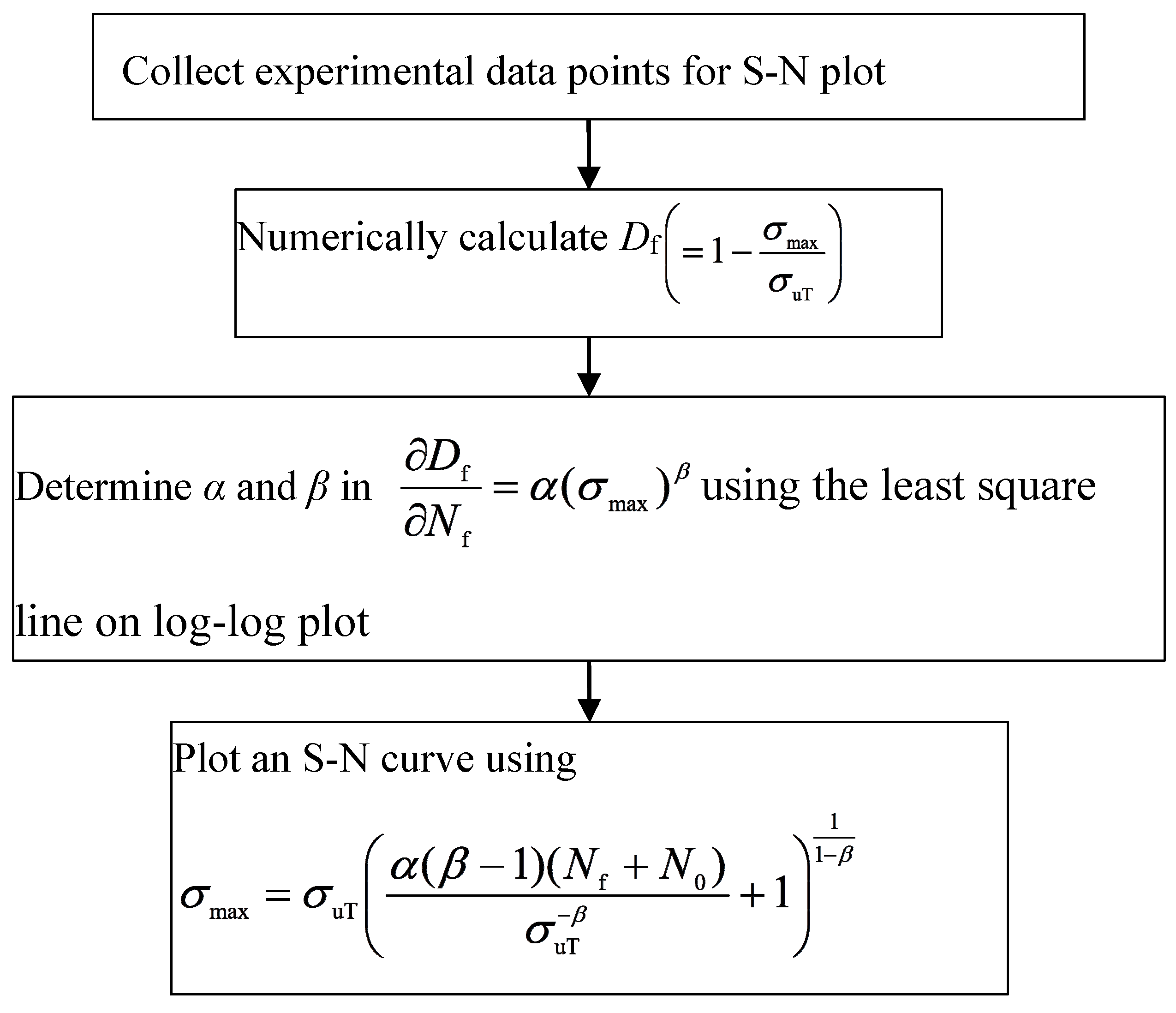
3.1. For Fatigue Data Characterisation
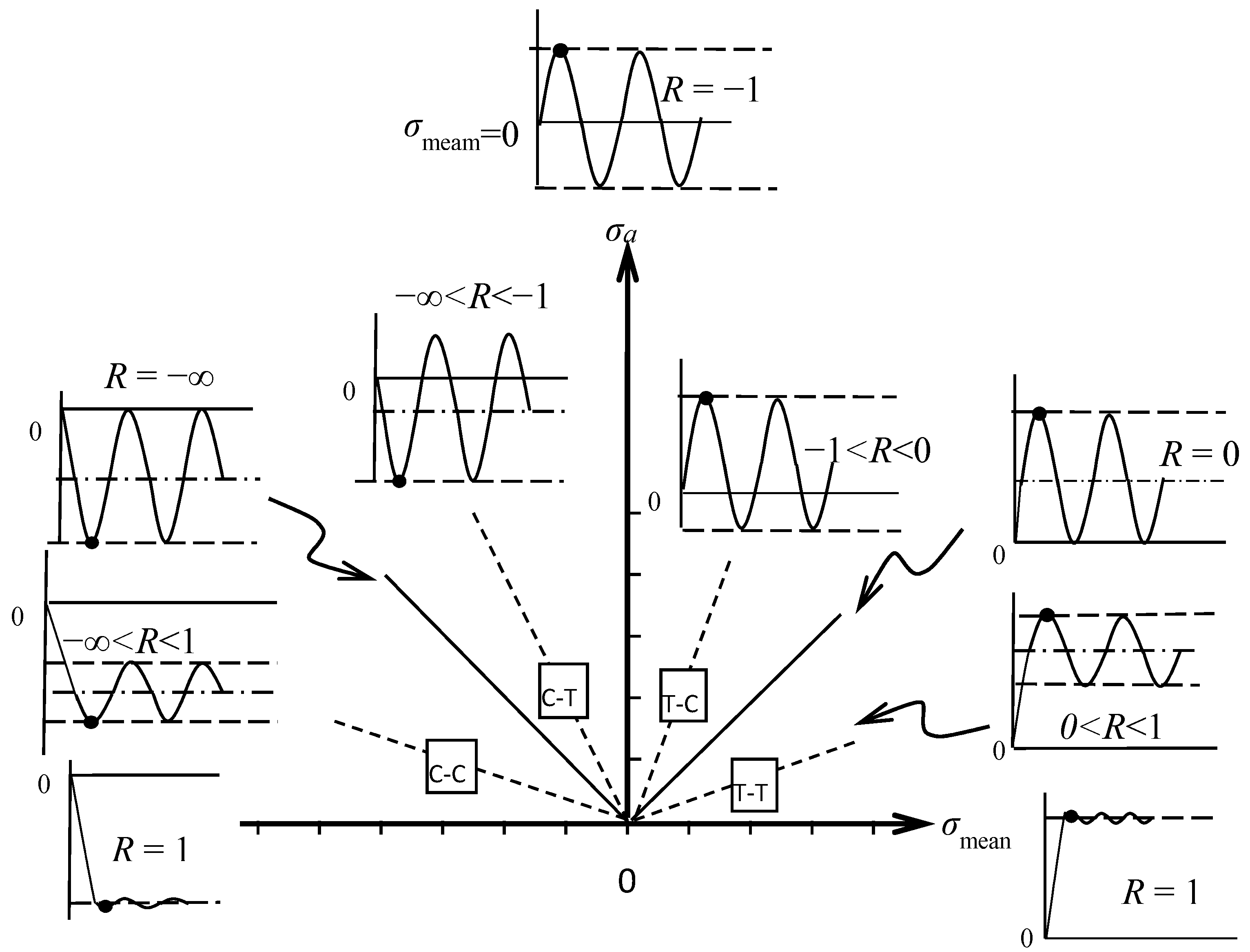
3.2. As a Function of Stress Ratio
3.3. Associated with Stress Intensity Factor
4. Evaluation of S-N Curve Model Capability
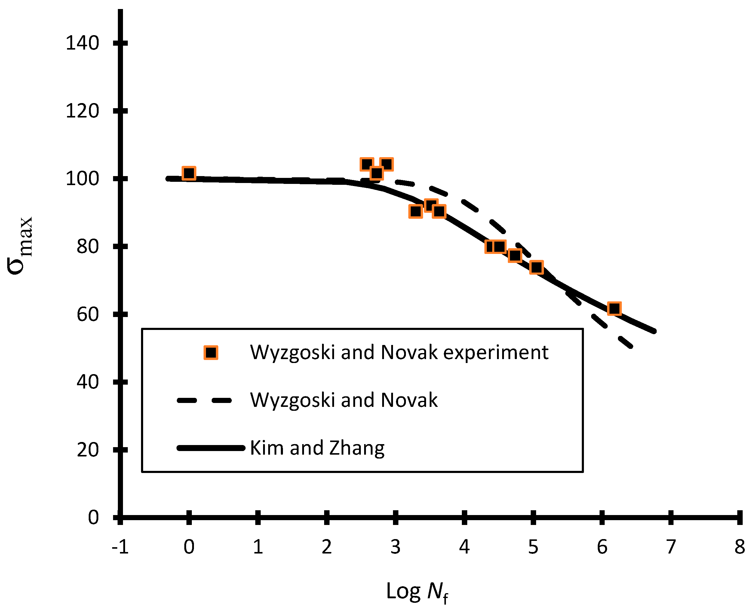
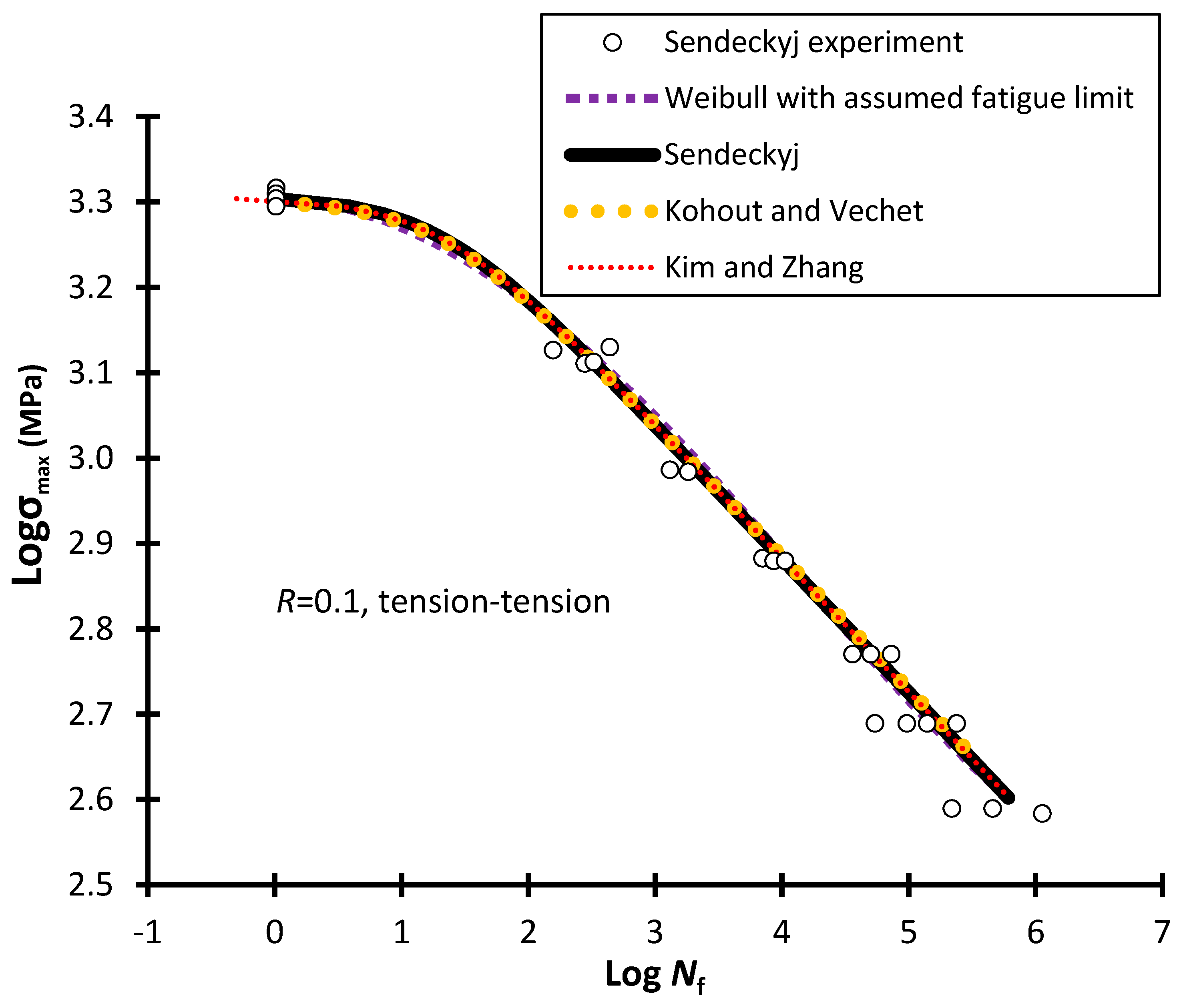
4.1. S-N Curve Models for Data Characterisation
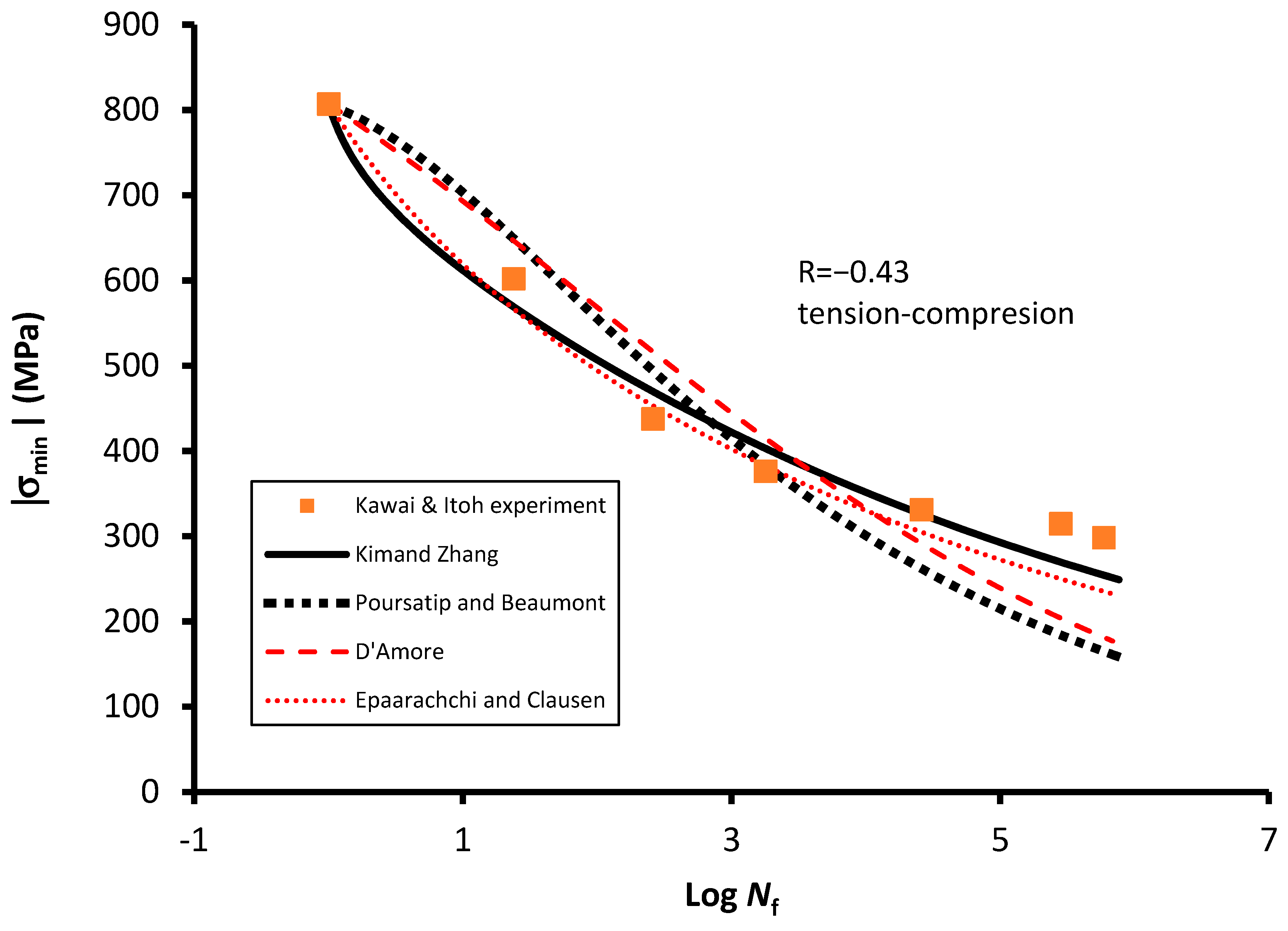
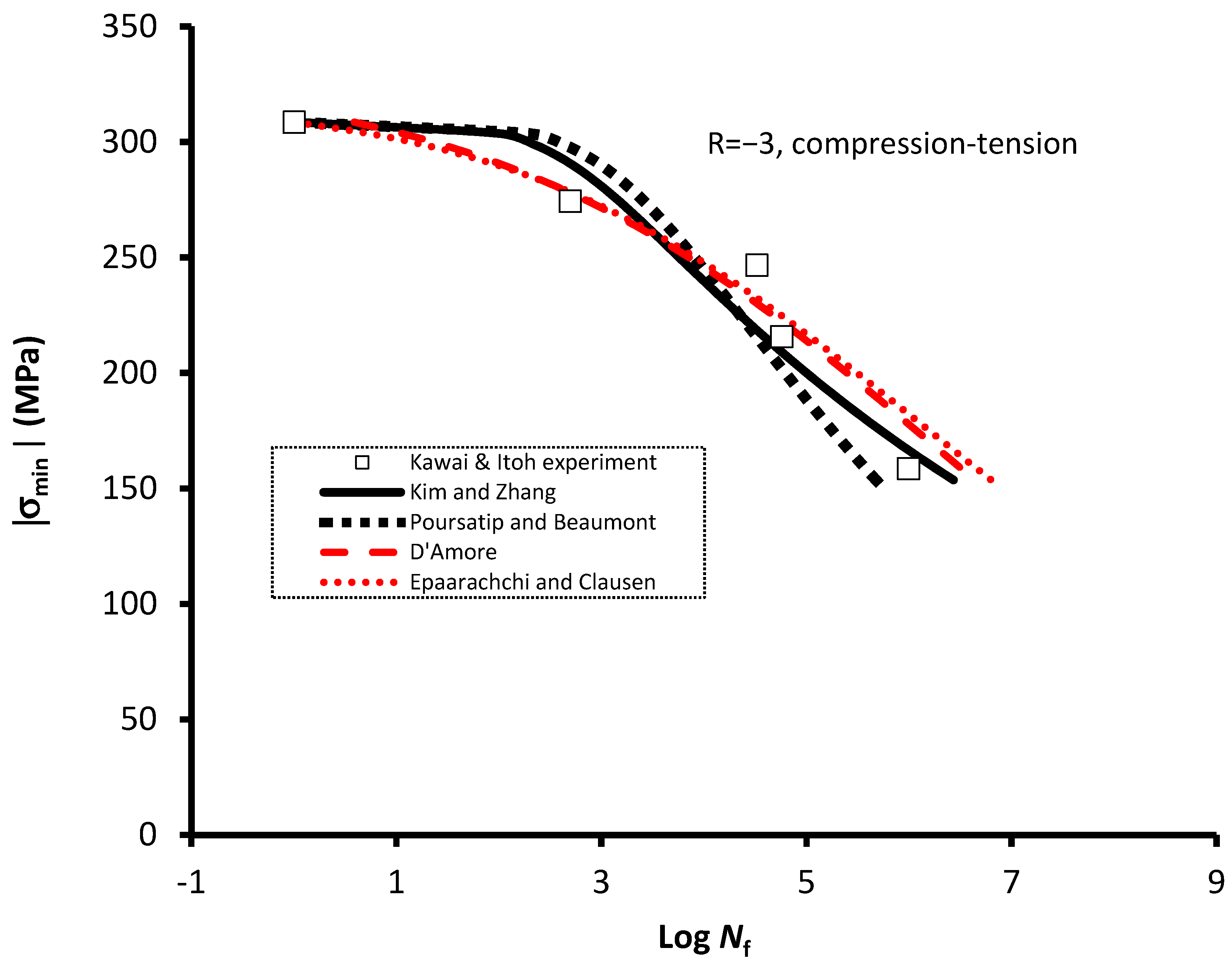
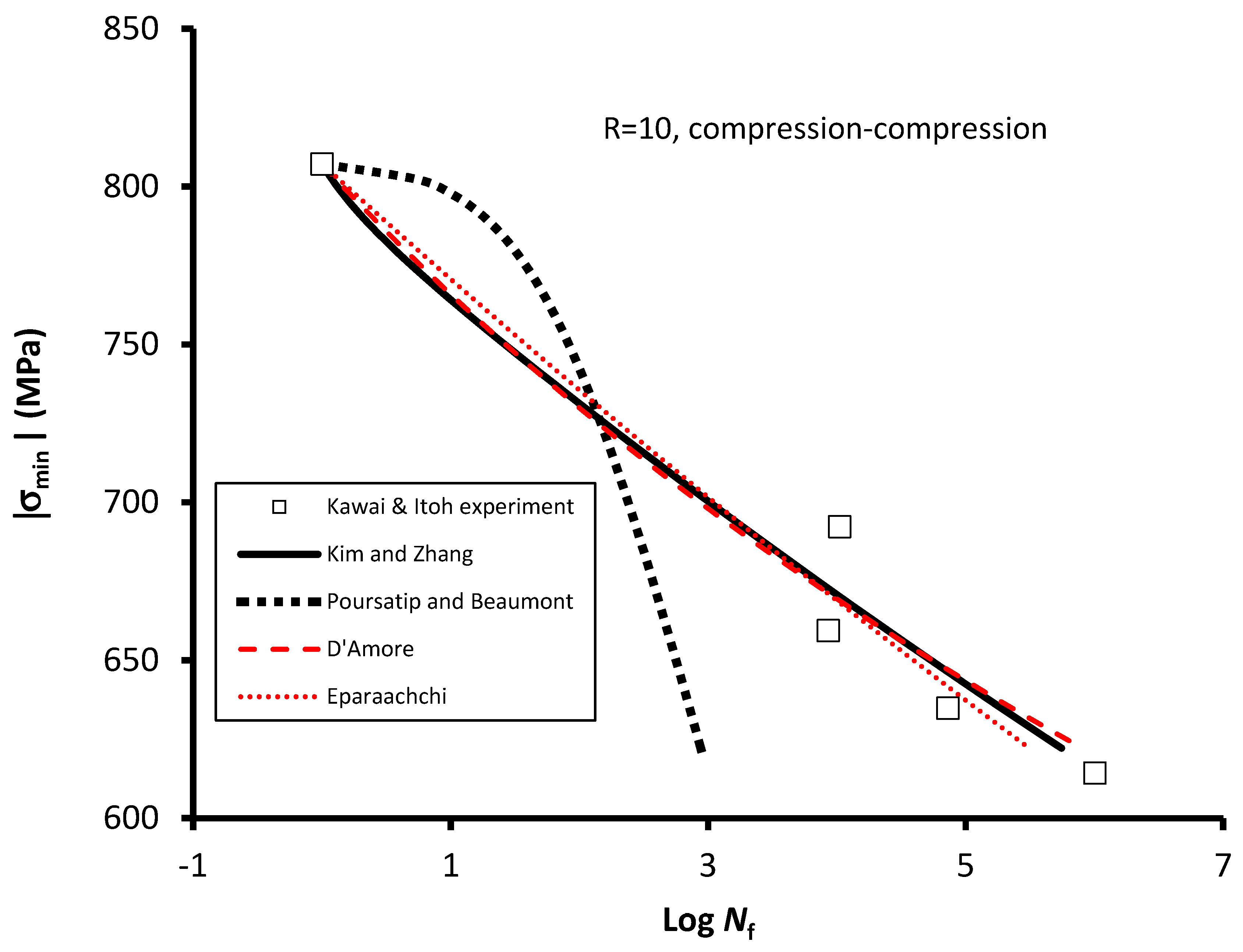
4.2. S-N Curve Models for Predicting Stress Ratio Effect
5. Conclusions
Funding
Acknowledgments
Conflicts of Interest
References
- Broek, D. Elementary Engineering Fracture Mechanics; Sijthoff & Noordhoff: Amsterdam, The Netherlands, 1978; ISBN 90-286-0208-9. [Google Scholar]
- Kitagawa, H.; Takashima, S. Application of fracture mechanics to very small fatigue cracks or the cracks in the early stage. In Proceedings of the Second International Conference on Mechanical Behavior of Materials, American Society for Metals, Materials Park, Boston, MA, USA, 16–20 August 1976; pp. 627–631. [Google Scholar]
- Weibull, W. A Statistical Distribution Function of wide Applicability. J Appl. Mech. 1951, 18, 293–297. [Google Scholar]
- Wang, S.S.; Chim, E.S.-M. Fatigue Damage and Degradation in Random Short-Fiber SMC Composite. J. Compos. Mater. 1983, 17, 114–134. [Google Scholar] [CrossRef]
- Kawai, M.; Hachinohe, A. Two-stress level fatigue of unidirectional fiber–metal hybrid composite: GLARE 2. Int. J. Fatigue 2002, 24, 567–580. [Google Scholar] [CrossRef]
- Kawai, M.; Saito, S. Off-axis strength differential effects in unidirectional carbon/epoxy laminates at different strain rates and predictions of associated failure envelopes. Compos. Part A 2009, 40, 1632–1649. [Google Scholar] [CrossRef]
- Rhines, F.N. Quantitative microscopy and fatigue mechanisms. In Fatigue Mechanisms, Proceedings of the ASTM-NBS-NSF Symposium, Kansas City, MO, USA, 21–22 May 1978; ASTM STP 675; Fong, J.T., Ed.; American Society for Testing and Materials: Philadelphia, PA, USA, 1979; pp. 23–46. [Google Scholar]
- Rupean, J.; Bhowal, P.; Eylon, D.; McEvily, A.J. On the process of subsurface fatigue crack initiation in Ti-6Al-4V. In Fatigue Mechanisms, Proceedings of the ASTM-NBS-NSF Symposium, Kansas City, MO, USA, 21–22 May 1978; ASTM STP 675; Fong, J.T., Ed.; American Society for Testing and Materials: Philadelphia, PA, USA, 1979; pp. 47–68. [Google Scholar]
- Karadag, M.; Stephens, R.I. The influence of high R ratio on unnotched fatigue behavior of 1045 steel with three different heat treatments. Int. J. Fatigue 2003, 25, 191–200. [Google Scholar] [CrossRef]
- Schütz, W. A history of fatigue. Eng. Fract. Mech. 1996, 54, 263–300. [Google Scholar] [CrossRef]
- Braithwaite, F. On the fatigue and consequent fracture of metals. In Minutes of the Proceedings of Civil Engineers; Institution of Civil Engineers: London, UK, 1854; Volume 13, pp. 463–467. [Google Scholar]
- Wöhler, A. Ueber die Festigkeits-Versuche mit Eisen und Stahl; Ernst & Korn: Berlin, German, 1870; pp. 74–106. [Google Scholar]
- Gerber, W.Z. Bestimmung der zulassigen Spannungen in Eisen-Constructionen. [Calculation of the allowable stresses in iron structures]. Z Bayer Arch. Ing. Ver. 1874, 6, 101–110. [Google Scholar]
- Weyrauch, P.J.J. Strength and Determination of the Dimensions of Structures of Iron and Steel with Reference to the Latest Investigations, 3rd ed.; Du Bois, A.J., Translator; John Wiley and Sons: New York, NY, USA, 1891. [Google Scholar]
- Goodman, J. Mechanics Applied to Engineering, 1st ed.; Longmans, Green and Co.: London, UK, 1899. [Google Scholar]
- Soderberg, C.R. Factor of safety and working stress. Trans. Am. Soc. Test Matls. 1930, 52, 13–28. [Google Scholar]
- Basquin, O.H. The exponential law of endurance test. ASTM STP 1910, 10, 625–630. [Google Scholar]
- Weibull, W. The statistical aspect of fatigue failures and its consequences. In Fatigue and Fracture of Metals; Massachusetts Institute of Technology; John Wiley & Sons: New York, NY, USA, 1952; pp. 182–196. [Google Scholar]
- Sendeckyj, G.P. Fitting models to composite materials fatigue data. In Test Methods and Design Allowables for Fibrous Composites; ASTM STP 734; Chamis, C.C., Ed.; ASTM International: West Conshohocken, PA, USA, 1981; pp. 245–260. [Google Scholar]
- Hwang, W.; Han, K.S. Cumulative damage models and multi-stress fatigue life prediction. J. Compos. Mater. 1986, 20, 125–153. [Google Scholar] [CrossRef]
- Kawai, M.; Koizumi, M. Nonlinear constant fatigue life diagrams for carbon/epoxy laminates at room temperature. Compos. Part A Appl. Sci. Manuf. 2007, 38, 2342–2353. [Google Scholar] [CrossRef]
- Kawai, M.; Itoh, N. A failure-mode based anisomorphic constant life diagram for a unidirectional carbon/epoxy laminate under off-axis fatigue loading at room temperature. J. Compos. Mater. 2014, 48, 571–592. [Google Scholar] [CrossRef]
- Palmgren, A. Die Lebensdauer von Kugellagern. Schwed Warmewirtschaft 1924, 68, 339–341. [Google Scholar]
- Hwang, W.; Han, K.S. Fatigue of Composites—Fatigue Modulus Concept and Life Prediction. J. Compos. Mater. 1986, 20, 154–165. [Google Scholar] [CrossRef]
- Poursartip, A.; Ashby, M.F.; Beaumont, P.W.R. The fatigue damage mechanics of carbon fibre composite laminate: I—Development of the model. Compos. Sci. Technol. 1986, 25, 193–218. [Google Scholar] [CrossRef]
- Poursartip, A.; Beaumont, P.W.R. The fatigue damage mechanics of carbon fibre composite laminate: II—Life prediction. Compos. Sci. Technol. 1986, 25, 283–299. [Google Scholar] [CrossRef]
- Eskandari, H.; Kim, H.S. A Theory for mathematical framework and fatigue damage function for the S-N plane. In Fatigue and Fracture Test Planning, Test Data Acquisitions, and Analysis; ASTM STP1598; Wei, Z., Nikbin, K., McKeighan, P.C., Harlow, D.G., Eds.; ASTM International: West Conshohocken, PA, USA, 2017; pp. 299–336. [Google Scholar]
- Mao, W.; Ringsberg, J.W.; Rychlik, I.; Li, Z. Theoretical development and validation of a fatigue model for ship routing. Ships Offshore Struct. 2012, 7, 399–415. [Google Scholar] [CrossRef]
- Miner, M.A. Cumulative damage in fatigue. Am. Soc. Mech. Eng. J. Appl. Mech. 1945, 12, 159–164. [Google Scholar]
- Philippidis, T.P.; Passipoularidis, V.A. Residual strength after fatigue in composites: Theory vs. experiment. Int. J. Fatigue 2007, 29, 2104–2116. [Google Scholar] [CrossRef]
- Post, N.; Case, S.; Lesko, J. Modeling the variable amplitude fatigue of composite materials: A review and evaluation of the state of the art for spectrum loading. Int. J. Fatigue 2008, 30, 2064–2086. [Google Scholar] [CrossRef]
- Eskandari, H.; Kim, H.S. A theory for mathematical framework of fatigue damage on S-N plane. Key Eng. Mater. 2015, 627, 117–120. [Google Scholar] [CrossRef]
- Rege, K.; Pavlou, D.G. A one-parameter nonlinear fatigue damage accumulation model. Int. J. Fatigue 2017, 98, 234–246. [Google Scholar] [CrossRef]
- Weibull, W. Chapter VIII, Presentation of Results. In Fatigue Testing and Analysis of Results; Pergaman Press: Oxford, UK; London, UK; New York, NY, USA; Paris, France, 1961. [Google Scholar]
- Kohout, J.; Vechet, S. A new function for fatigue curves characterization and its multiple merits. Int. J. Fatigue 2001, 23, 175–183. [Google Scholar] [CrossRef]
- Nijssen, R.P.L. Phenomenological fatigue analysis and life modelling. In Fatigue Life Prediction of Composites and Composite Structures; Vassilopolos, A.P., Ed.; Woodhead publishing Limited: Oxford, UK; Cambridge, UK; New Delhi, India, 2010; pp. 45–78. [Google Scholar]
- Xiong, J.J.; Shenoi, R.A. Fatigue and Fracture Reliability Engineering; Springer: London, UK; Dordrecht, The Netherlands; Heidelberg, German; New York, NY, USA, 2011. [Google Scholar]
- Burhan, I.; Kim, H.S.; Thomas, S. A refined S-N curve model. In Proceedings of the International Conference on Sustainable Energy, Environment and Information (SEEIE 2016), Bangkok, Thailand, 20–21 March 2016; pp. 412–416. [Google Scholar]
- Passipoularidis, V.A.; Philippidis, T.P.; Brondsted, P. Fatigue life prediction in composites using progressive damage modelling under block and spectrum loading. Int. J. Fatigue 2011, 33, 132–144. [Google Scholar] [CrossRef]
- Fatemi, A.; Yang, L. Cumulative fatigue damage and life prediction theories: A survey of the state of the art for homogeneous materials. Int. J. Fatigue 1998, 23, 9–34. [Google Scholar] [CrossRef]
- Yang, L.; Fatemi, A. Cumulative Fatigue Damage Mechanisms and Quantifying Parameters: A Literature Review. J. Test. Eval. 1998, 26, 89–100. [Google Scholar]
- Bathias, C.; Pineau, A. Fatigue of Materials and Structures-Application to Design and Damage; ISTE: London, UK; Wiley: Hoboken, NJ, USA, 2011. [Google Scholar]
- Christian, L. Chapter 2, Fatigue Damage. In Mechanical Vibration and Shock Analysis, 3rd ed.; John Wiley & Sons: London, UK; Hoboken, NJ, USA, 2014; Volume 4. [Google Scholar]
- O’Brian, T.K.; Reifsnider, K.L. Fatigue damage evaluation through stiffness measurements in boron-epoxy laminates. J. Compos. Mater. 1981, 15, 55–70. [Google Scholar]
- Marin, J. Mechanical Behavior of Engineering Materials; Prentice-Hall: Englewood Cliffs, NJ, USA, 1962. [Google Scholar]
- Subramanyan, S. A cumulative damage rule based on the knee point of the SN curve. J. Eng. Mater. Technol. 1976, 98, 316–321. [Google Scholar] [CrossRef]
- Mandell, J.F.; Meier, U. Effects of stress ratio, frequency, and loading time on the tensile fatigue of glass-reinforced epoxy. In Long-Term Behavior of Composites; ASTM STP 813; O’Brien, T.K., Ed.; American Society for Testing and Materials: Philadelphia, PA, USA, 1983; pp. 55–77. [Google Scholar]
- Bond, I.P.; Farrow, I.R. Fatigue life prediction under complex loading for XAS/914 CFRP incorporating a mechanical fastener. Int. J. Fatigue 2000, 22, 633–644. [Google Scholar] [CrossRef]
- Tamuz, V.; Dzelzitis, K.; Reifsnider, K. Fatigue of Woven Composite Laminates in Off-Axis Loading II. Prediction of the Cyclic Durability. Appl. Compos. Mater. 2004, 11, 281–292. [Google Scholar] [CrossRef]
- Gathercole, N.; Reiter, H.; Adam, T.; Harris, B. Life prediction for fatigue of T800/5245 carbon-fibre composites: I. Constant-amplitude loading. Fatigue 1994, 16, 523–532. [Google Scholar] [CrossRef]
- Adam, T.; Gathercole, N.; Reiter, H.; Harris, B. Life prediction for fatigue of T800/5245 carbon-fibre composites: II. Variable amplitude loading. Fatigue 1994, 16, 533–547. [Google Scholar] [CrossRef]
- Beheshty, M.H.; Harris, B.; Adam, T. An empirical fatigue-life model for high-performance fibre composites with and without impact damage. Compos. Part A Appl. Sci. Manuf. 1999, 30, 971–987. [Google Scholar] [CrossRef]
- Bathias, C. There is no infinite fatigue life in metallic materials. Fatigue Fract. Eng. Mater. Struct. 1999, 22, 559–565. [Google Scholar] [CrossRef]
- Stromeyer, C.E. The Determination of Fatigue Limits under Alternating Stress Conditions. Proc. R. Soc. A Math. Phys. Eng. Sci. 1914, 90, 411–425. [Google Scholar] [CrossRef] [Green Version]
- Henry, D.L. A Theory of Fatigue-Damage Accumulation in Steel. Trans. ASME 1955, 913–918. [Google Scholar]
- Ellyin, F. Cyclic Strain Energy Density as a Criterion for Multiaxial Fatigue Failure, Biaxial and Multiaxial Fatigue, EGF2; Brown, M.W., Miller, K.J., Eds.; Mechanical Engineering Publications: London, UK, 1989; pp. 571–583. [Google Scholar]
- Ellyin, F.; El-Kadi, H. A fatigue failure criterion for fibre reinforced composite laminae. Compos. Struct. 1990, 15, 61–74. [Google Scholar] [CrossRef]
- Kensche, C.W. Influence of composite fatigue properties on lifetime predictions of sailplanes. In Proceedings of the XXIV OSTIV Congress, Vol XIX, No 3, Omarama, New Zealand, 12–19 January 1995; pp. 69–76. [Google Scholar]
- Kulawinski, D.; Kolmorgen, R.; Biermann, H. Application of Modified Stress_Strain Approach for the Fatigue-Life Prediction of a Ferritic, an Austenitic and a Ferritic-Austenitic Duplex Steel under Isothermal and Thermo-Mechanical Fatigue. Steel Res. Int. 2016, 87, 1095–1104. [Google Scholar] [CrossRef]
- Kim, H.S.; Zhang, J. Fatigue Damage and Life Prediction of Glass/Vinyl Ester Composites. J. Reinf. Plast. Compos. 2001, 20, 834–848. [Google Scholar] [CrossRef]
- Kassapoglou, C. Fatigue life prediction of composite structures under constant amplitude loading. J. Compos. Mater. 2007, 41, 2737–2754. [Google Scholar] [CrossRef]
- Kassapoglou, C. Fatigue of composite materials under spectrum loading. Compos. Part A 2010, 41, 663–669. [Google Scholar] [CrossRef]
- Owen, M.; Howe, R. The accumulation of damage in a glass-reinforced plastic under tensile and fatigue loading. J. Phys. D Appl. Phys. 1972, 5, 1637–1649. [Google Scholar] [CrossRef]
- Yang, J.N.; Liu, M.D. Residual Strength Degradation Model and Theory of Periodic Proof Tests for Graphite/Epoxy Laminates. J. Compos. Mater. 1977, 11, 176–203. [Google Scholar] [CrossRef]
- Yang, J.N. Fatigue and Residual Strength Degradation for Graphite/Epoxy Composites Under Tension-Compression Cyclic Loadings. J. Compos. Mater. 1978, 12, 19–39. [Google Scholar] [CrossRef]
- Rotem, A. Residual Strength after Fatigue Loading. Int. J. Fatigue 1988, 10, 27–31. [Google Scholar] [CrossRef]
- D’Amore, A.; Caprino, G.; Stupak, P.; Zhou, J.; Nicolais, L. Effect of stress ratio on the flexural fatigue behaviour of continuous strand mat reinforced plastics. Sci. Eng. Compos. Mater. 1996, 5, 1–8. [Google Scholar] [CrossRef]
- Caprino, G.; Giorlea, G. Fatigue lifetime of glass fabric/epoxy composites. Compos. Part A Appl. Sci. Manuf. 1999, 30, 299–304. [Google Scholar] [CrossRef]
- Epaarachchi, J.A.; Clausen, P.D. An empirical model for fatigue behavior prediction of glass fibre-reinforced plastic composites for various stress ratios and test frequencies. Compos. Part A Appl. Sci. Manuf. 2003, 34, 313–326. [Google Scholar] [CrossRef]
- Epaarachchi, J.A. Effects of static-fatigue (tension) on the tension-tension fatigue life of glass fibre reinforced plastic composites. Compos. Struct. 2006, 74, 419–425. [Google Scholar] [CrossRef]
- Wyzgoski, M.G.; Novak, G.E. Predicting fatigue S-N (stress-number of cycles to fail) behavior of reinforced plastics using fracture mechanics theory. J. Mater. Sci. 2005, 40, 295–308. [Google Scholar] [CrossRef]
- Paris, P.; Erdogan, F. A critical Analysis of Crack Propagation Laws. Trans. ASME 1963, 85, 528–534. [Google Scholar] [CrossRef]
- Wyzgoski, M.G.; Novak, G.E. An improved model for predicting fatigue S–N (stress–number of cycles to fail) behavior of glass fiber reinforced plastics. J. Mater. Sci. 2008, 43, 2879–2888. [Google Scholar] [CrossRef]
- Murakami, Y. Stress Intensity Factors Handbook; Pergamon Press: Oxford, UK, 1987. [Google Scholar]
- Bond, I.P.; Ansell, M.P. Fatigue properties of jointed wood composites-Part I Statistical analysis, fatigue master curves and constant life diagrams. J. Mater. Sci. 1998, 33, 2751–2762. [Google Scholar] [CrossRef]
- Li, Z.; Zou, H.; Dai, J.; Feng, X.; Sun, M.; Peng, L. A comparison of low-cycle fatigue behavior between the solutionized and aged Mg-3Nd-0.2Zn-0.5Zr alloys. Mater. Sci. Eng. 2017, 695, 342–349. [Google Scholar] [CrossRef]
- Liu, Y.B.; Li, Y.D.; Li, S.X.; Yang, Z.G.; Chen, S.M.; Hui, W.J.; Weng, Y.Q. Prediction of the S–N curves of high-strength steels in the very high cycle fatigue regime. Int. J. Fatigue 2010, 32, 1351–1357. [Google Scholar] [CrossRef]


| S-N Curve Models | Capability of Curve Fitting | Adaptability to Different Stress Ratios | Relation with Physical Properties | Remarks | ||
|---|---|---|---|---|---|---|
| Boundary at Initial Nf | Damage Representation | Satisfaction of | ||||
| Basquin (1910) | Poor | Poor | N/A | N/A | N/A | |
| Stromeyer (1914) | Poor | Poor | N/A | N/A | N/A | |
| Weibull (1952) | Good | Good | Yes | N/A | N/A | Fatigue limit is required |
| Henry (1955) | Poor | N/A | N/A | N/A | N/A | |
| Marin (1962) | Poor | N/A | N/A | N/A | N/A | Same form as Basquin model. |
| Sendeckyj (1981) | Good | Good | Yes | N/A | N/A | |
| Hwang and Han (1986) | Poor | Poor | No | N/A | N/A | |
| Kohout and Vechet (2001) Equation (19) | Good | Good | No | N/A | N/A | With limited curve shaping (e.g., R = −0.43) |
| Kim and Zhang (2001) | Good | Good | Yes | Yes | Yes | |
| Experimental Data | Loading | S-N Curve Models | Fitting Parameters | |||
|---|---|---|---|---|---|---|
| α | β | σ∞ (MPa) | N0 | |||
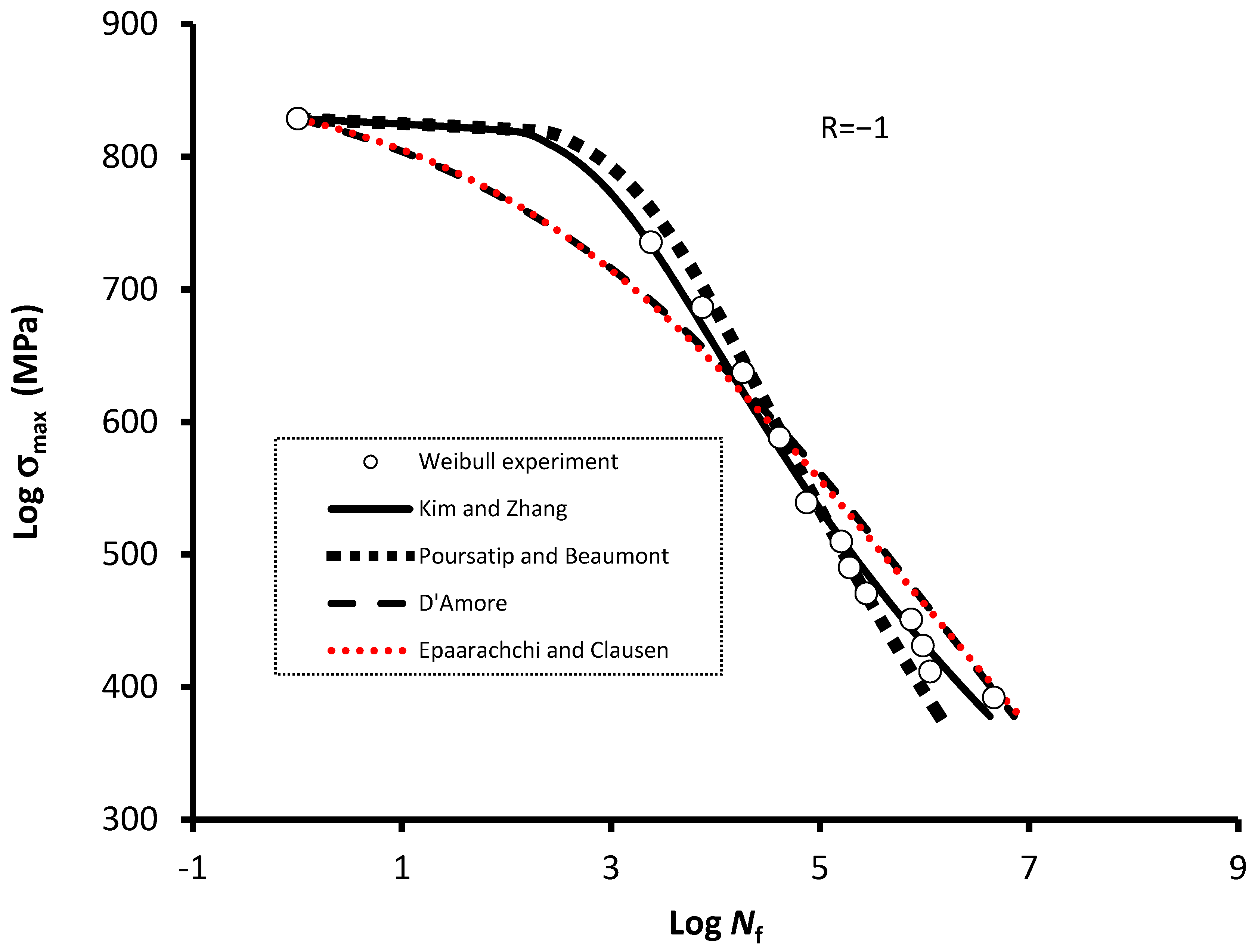
| Weibull (1952) [18] with σuT = 829 MPa | R = −1 for T-C or C-T loading | Weibull (1952) | 2.1 × 10⁻⁵ | 3.8 | 353 | - |
| 0.003 | 3.1 | 0 | - | |||
| Sendeckyj (1981) | 0.001 | 0.093 | - | - | ||
| Kohout and Vechet (2001) | 776.25 | −0.090 | - | - | ||
| Kim and Zhang (2001) | 10−38.44 | 11.81 | - | 0.5 | ||
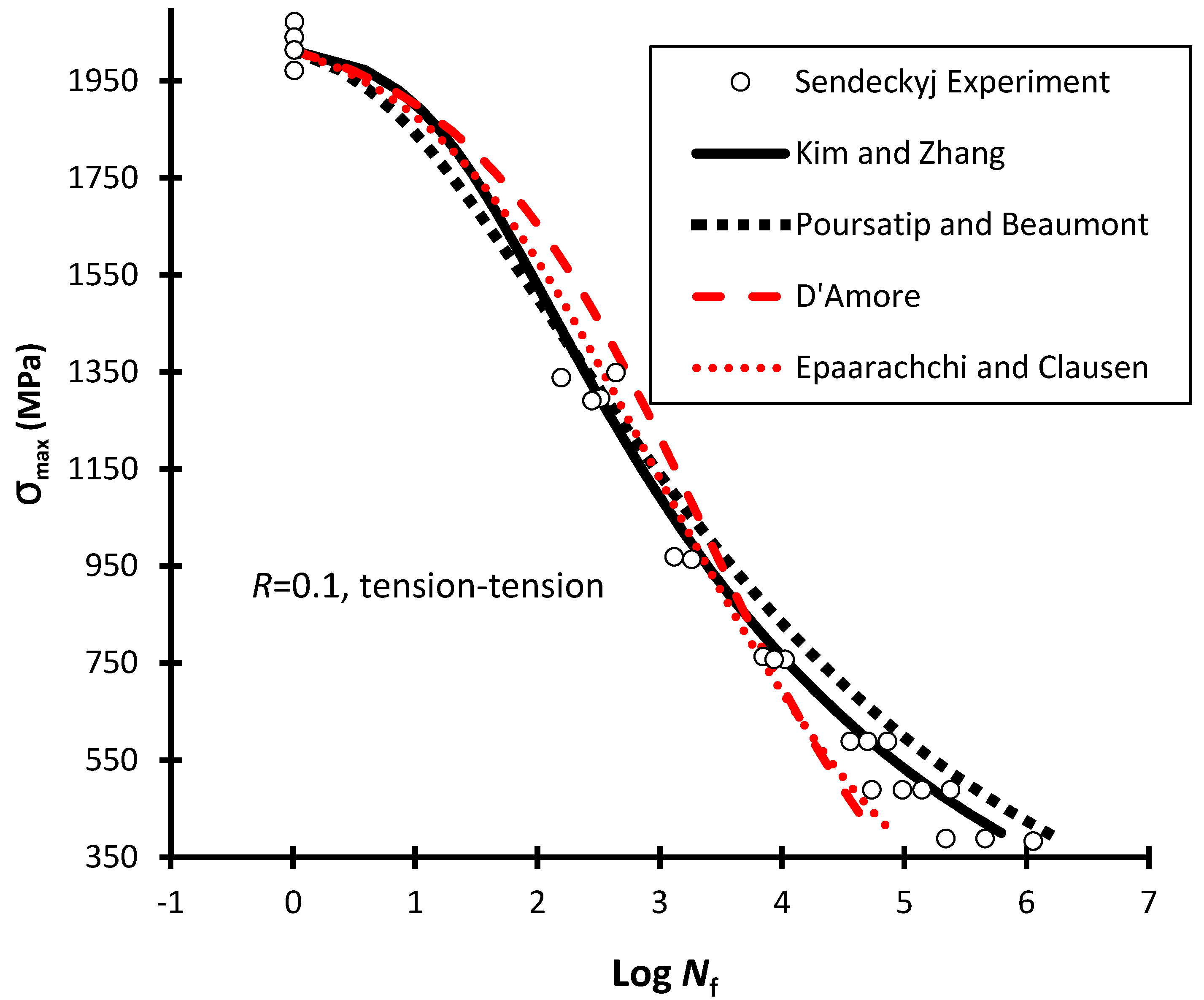
| Sendeckyj (1981) [19] σuT = 2013 MPa | R = 0.1 for T-T loading | Weibull (1952) | 0.088 | 1.9 | 250 | - |
| Sendeckyj (1981) | 0.0485 | 0.157 | - | - | ||
| Kohout and Vechet (2001) | 19.953 | −0.155 | - | |||
| Kim and Zhang (2001) | 3.13 × 10⁻²⁷ | 7.381 | - | 0.5 | ||
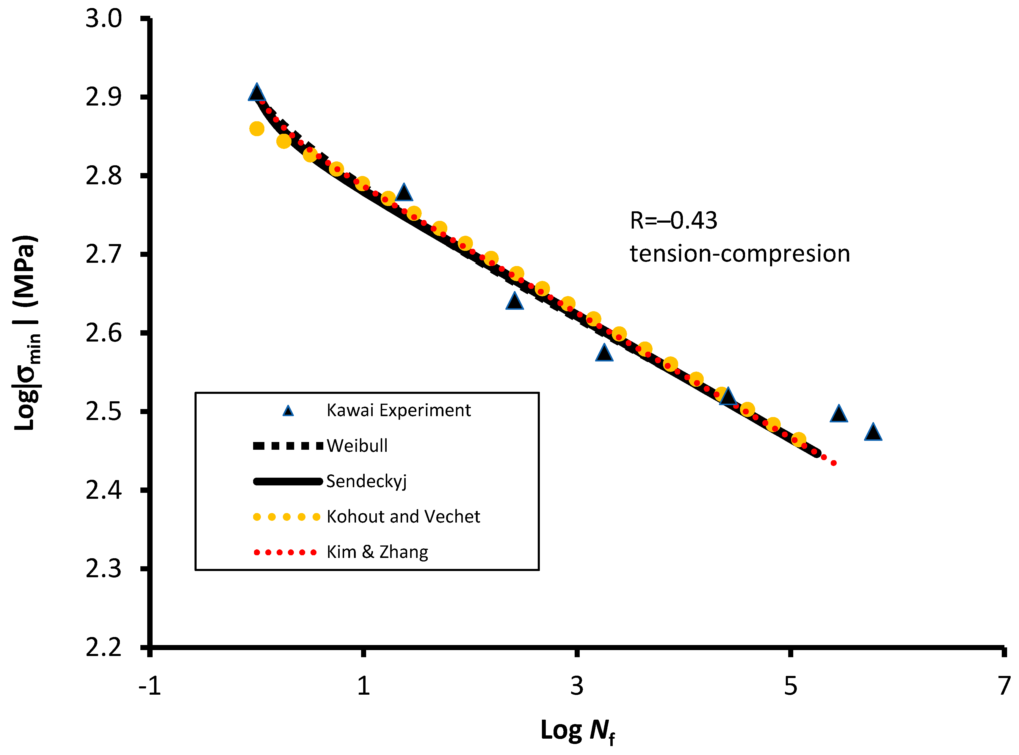
| Kawai and Itoh (2014) [22] with σuC = 807 and σuT = 1887 MPa | R = −0.43 for T-C loading | Weibull | 2.5 × 10⁻¹ | 0.83 | 0 | 1 |
| Sendeckyj (1981) | 4.485 | 0.078 | - | 1 | ||
| Kohout and Vechet (2001) | 0.35 | −0.08 | - | - | ||
| Kim and Zhang (2001) | 2.88 × 10−160 | 54.39 | - | 1 | ||
| Kawai and Itoh (2014) [22] with σuC = 807MPa and σuT = 1887 MPa | R = −3 for C-T loading | Weibull (1952) | 3.5 × 10⁻³ | 3.59 | 150 | - |
| Sendeckyj (1981) | 1.985 × 10⁻³ | 0.08 | - | - | ||
| Kohout and Vechet (2001) | 398.1 | −7.75 × 10⁻² | - | - | ||
| Kim and Zhang (2001) | 4.295 × 10−38 | 13.506 | - | 0.5 | ||
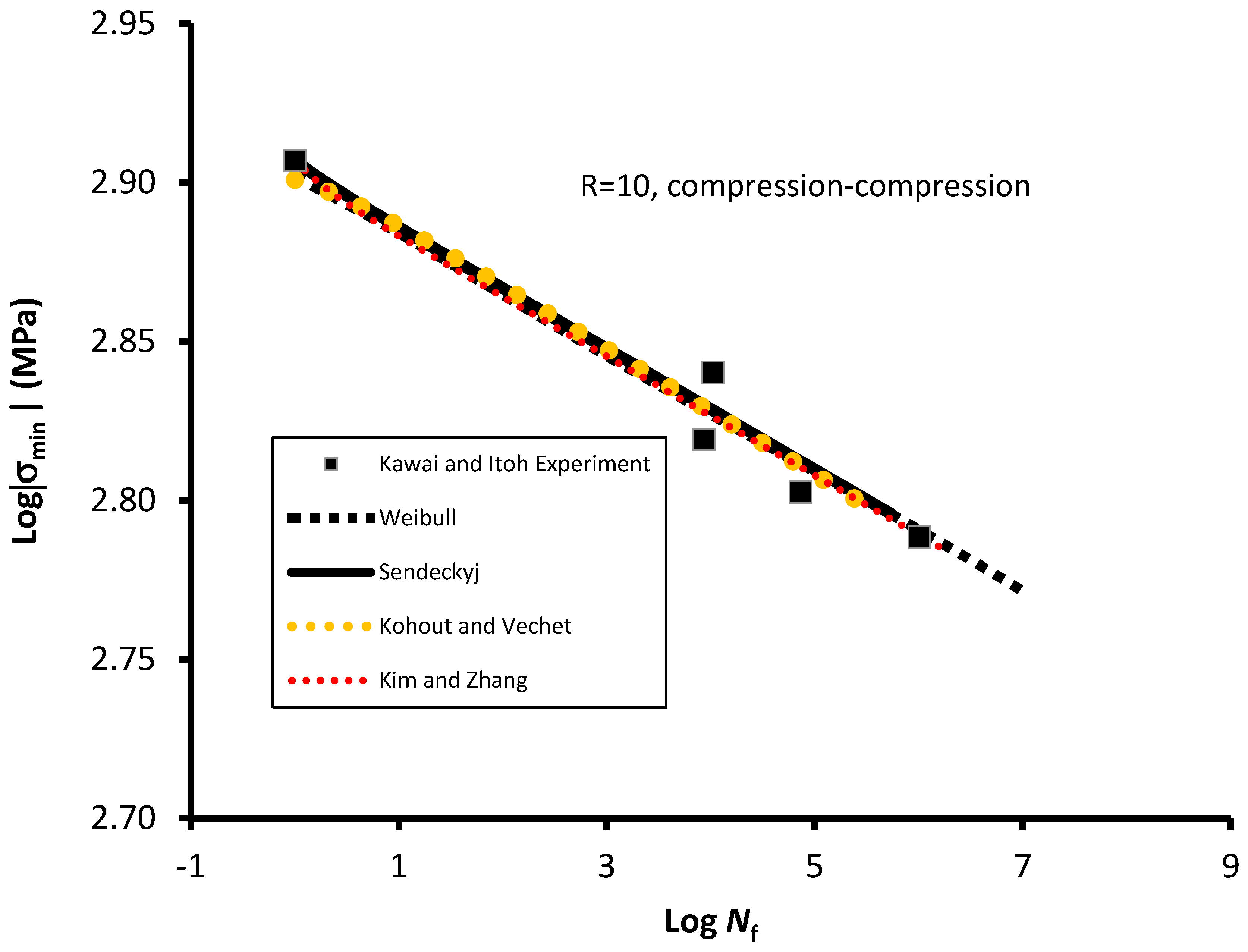
| Kawai and Itoh (2014) [22] with σuC = 807 MPa and σuT = 1887 MPa | R = 10 for C-C loading | Weibull (1952) | 0.138 | 0.66 | 185 | 1 |
| Sendeckyj (1981) | 1.3 | 0.019 | - | 1 | ||
| Kohout and Vechet (2001) | 1 | −0.02 | - | - | ||
| Kim and Zhang (2001) | 2.88 × 10−160 | 54.388 | - | 1 | ||
| S-N Models | Google Scholar Citations | Citation Rates/Year |
|---|---|---|
| Basquin (1910) | 1311 | 12 |
| Weibull (1952) | 14 | 0.21 |
| Sendeckyj (1981) | 111 | 3.0 |
| Kohout and Vechet (2001) | 73 | 4.3 |
| Kim and Zhang (2001) | 15 | 0.88 |
| S-N Curve Models | Capability of Curve Fitting and Applicability to Different Stress Ratios | Number of Fitting Parameters | Relation with Physical Properties | |||
|---|---|---|---|---|---|---|
| Boundary at Initial Nf | Damage Representation | Satisfaction of | ||||
| R | Capability | |||||
| Poursartip and Beaumont (1986) | 1 | Good | 1 | Yes | Partially Yes | Yes |
| 0.1 | Good | |||||
| −0.43 | Poor | |||||
| −3 | Reasonable | |||||
| 10 | Poor | |||||
| D’Amore et al. (1996) | −1 | Poor | 2 | Yes | N/A | N/A |
| 0.1 | Reasonable | |||||
| −0.43 | Poor | |||||
| −3 | Reasonable | |||||
| 10 | Good | |||||
| Epaarachchi and Clausen (2003) | −1 | Poor | 2 | Yes | N/A | N/A |
| 0.1 | Reasonable | |||||
| −0.43 | Good | |||||
| −3 | Reasonable | |||||
| 10 | Good | |||||
© 2018 by the authors. Licensee MDPI, Basel, Switzerland. This article is an open access article distributed under the terms and conditions of the Creative Commons Attribution (CC BY) license (http://creativecommons.org/licenses/by/4.0/).
Share and Cite
Burhan, I.; Kim, H.S. S-N Curve Models for Composite Materials Characterisation: An Evaluative Review. J. Compos. Sci. 2018, 2, 38. https://doi.org/10.3390/jcs2030038
Burhan I, Kim HS. S-N Curve Models for Composite Materials Characterisation: An Evaluative Review. Journal of Composites Science. 2018; 2(3):38. https://doi.org/10.3390/jcs2030038
Chicago/Turabian StyleBurhan, Ibrahim, and Ho Sung Kim. 2018. "S-N Curve Models for Composite Materials Characterisation: An Evaluative Review" Journal of Composites Science 2, no. 3: 38. https://doi.org/10.3390/jcs2030038