Reactive Molecular Dynamics Study of the Thermal Decomposition of Phenolic Resins
by
 , and
, and
Marcus Purse
1, 
Grace Edmund
1,
Stephen Hall
1,
Brendan Howlin
1,*,
Ian Hamerton
2 and
and
Stephen Till
3 1
Department of Chemistry, Faculty of Engineering and Physical Sciences, University of Surrey, Guilford, Surrey GU2 7XH, UK
2
Bristol Composites Institute (ACCIS), Department of Aerospace Engineering, School of Civil, Aerospace, and Mechanical Engineering, University of Bristol, Bristol BS8 1TR, UK
3
Defence Science and Technology Laboratory, Porton Down, Salisbury SP4 0JQ, UK
*
Author to whom correspondence should be addressed.
J. Compos. Sci. 2019, 3(2), 32; https://doi.org/10.3390/jcs3020032
Submission received: 6 March 2019
/
Revised: 21 March 2019
/
Accepted: 23 March 2019
/
Published: 28 March 2019
(This article belongs to the Special Issue Durability of Composites Under Severe Environmental Conditions)
Abstract
:The thermal decomposition of polyphenolic resins was studied by reactive molecular dynamics (RMD) simulation at elevated temperatures. Atomistic models of the polyphenolic resins to be used in the RMD were constructed using an automatic method which calls routines from the software package Materials Studio. In order to validate the models, simulated densities and heat capacities were compared with experimental values. The most suitable combination of force field and thermostat for this system was the Forcite force field with the Nosé–Hoover thermostat, which gave values of heat capacity closest to those of the experimental values. Simulated densities approached a final density of 1.05–1.08 g/cm3 which compared favorably with the experimental values of 1.16–1.21 g/cm3 for phenol-formaldehyde resins. The RMD calculations were run using LAMMPS software at temperatures of 1250 K and 3000 K using the ReaxFF force field and employing an in-house routine for removal of products of condensation. The species produced during RMD correlated with those found experimentally for polyphenolic systems and rearrangements to form cyclopropane moieties were observed. At the end of the RMD simulations a glassy carbon char resulted.
1. Introduction
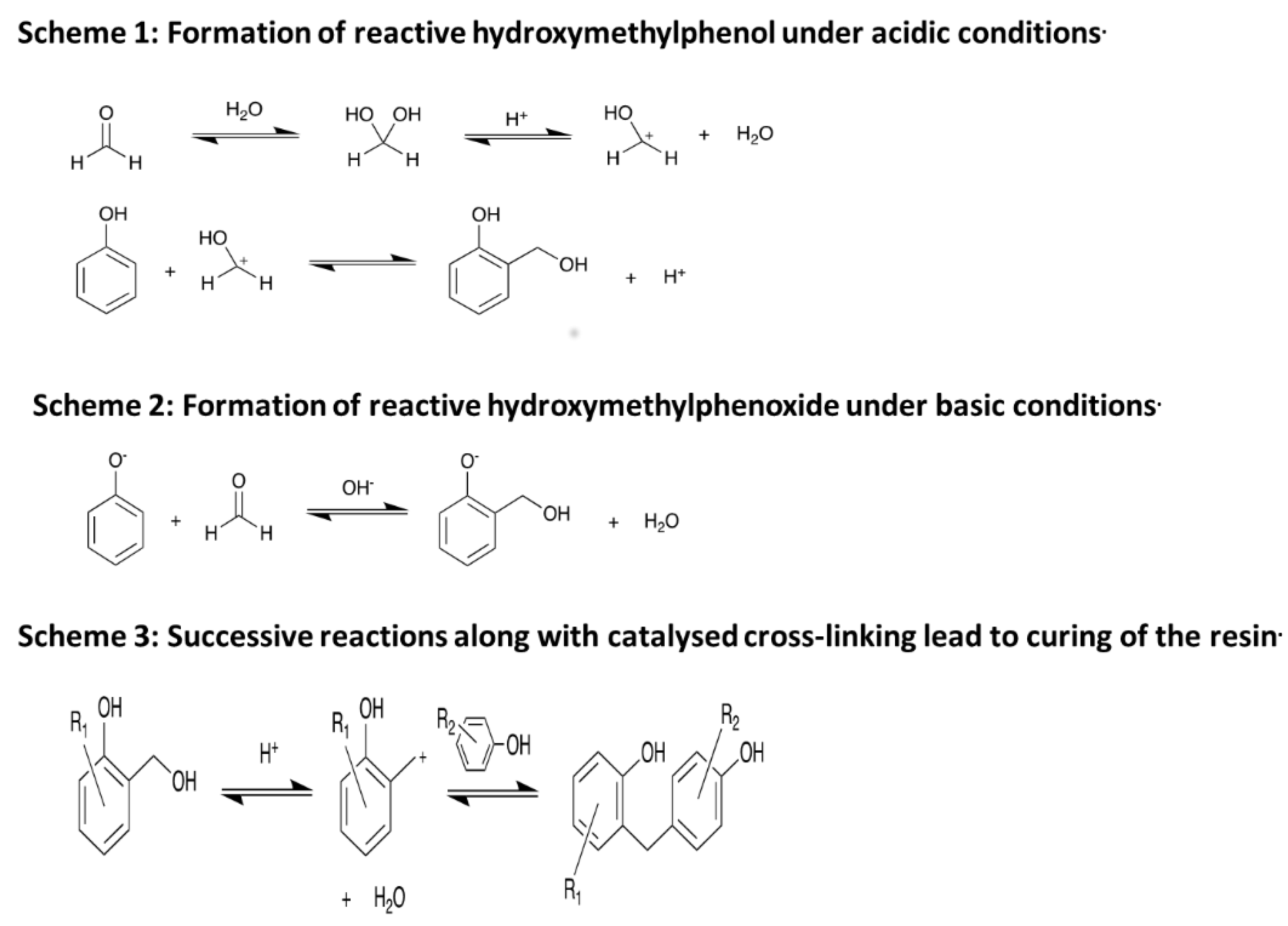
The field of reactive molecular dynamics of polymers has progressed considerably since the review by Lyon et al. in 2003 that studied models consisting of 20 monomer chains of the polymers under investigation [1]. There have been several papers on reactive molecular dynamics (RMD) of bituminous coal in particular. Bhoi, Banerjee, and Mohanty [2] studied the combustion and pyrolysis of brown coal by RMD, and they concluded that hydrogen was abstracted to form water and that the levels of simulated formaldehyde agreed with the experimental literature. Zan et al. [3] studied the initial reaction of sub-bituminous coal using RMD and Illinois no. 6 coal was simulated in a study by van Duin et al. [4]. Most relevant to this work, Liu at al. [5] studied the pyrolysis of high-density polyethylene using RMD and a model of 7000 atoms and they found that the reaction time for 90% of the loss of structure agreed with the experimental values. This study used a new graphical interface to help interpret the results [6]. An interesting study [7] used RMD to probe the oxidation resistance in hydrogen peroxide of ultra-high molecular weight polyethylene and polyoxymethylene. Two recent studies looked at energetic materials [8,9] and composites featured in a study of carbon nanofiber supported particles [10], graphene sheets [11], and lignite [12]. Tetrabutylphosphonium glycinate/CO2 mixtures were also investigated by van Duin [13]. A new force field was derived for Pt-O systems by Fantauzzi et al. [14], and an organic mechanistic study was carried out on polymerization by Schoenfelder [15]. Adaptive accelerated RMD on hydrogen was published by Goddard et al. [16], and an implementation of RMD on GPU’s was developed by Kylasa et al. [17]. The second generation of RMD methods were reviewed by Farah et al. in 2012 [18], which used empirical reactive force fields to generate the new species. Recently, a transferable reactive force field was developed by Xiao, Shi, Hao, Liao, Zhang, and Chen for phosphorous and hydrogen which showed a distinct improvement in predicting the mechanical properties of pristine- and defect-laden black phosphorous [19]. In this study we concentrate on phenol-formaldehyde resins (PFRs), also known as phenolic resins, which are a subclass of synthetically derived thermosetting polymers obtained from a reaction of phenol with formaldehyde (Figure 1).
Although substituted derivatives of either may also be used [20], under aqueous acidic conditions formaldehyde reacts with water to form methylene glycol, a difunctional monomer that is the key to linking the phenol units. A 0.8:1 mixture of phenol and methylene glycol produces an alternating copolymer, known as a novolac, with only a small amount of branching. The addition of a hardener, hexamethylenetetramine, crosslinks the novolac prepolymers, forming the thermoset [20]. Under aqueous basic conditions, phenol is converted to the phenoxide ion which is substituted in the ortho- or para-positions by a formaldehyde molecule. A 1.5:1 mixture of formaldehyde and phenol is used along with water and a suitable catalyst. These reactants are heated to produce a prepolymer which is rich in hydroxymethylphenols [20]. Further heating of this prepolymer causes reactions of the hydroxymethyl groups with other phenols to form large cross-linked structures, known as resoles, without the need for a hardener [20]. PFRs have found a wide variety of uses in the modern world ranging from work surfaces to circuit boards to billiard balls. They have been utilized by the aerospace industry to construct ablative heat shields for space vehicles which work by charring and subliming on re-entry. The expulsion of gaseous pyrolysis products creates a comparatively cool cushion of gas that protects the vehicle from the hot shock gas layer. These PFR-based heat shields have been used by both the National Aeronautics and Space Administration (NASA) and the Soviet Union [21]. When possible, it is important that a model reproduces experimental parameters, and in particular as in this case, when the model is going to be used to study decomposition. There is a wide range of experimental comparisons that can be used, e.g., density, elastic moduli, and glass transition temperature, many of which we have previously reported [22]. Because we were interested in decomposition, in this study the simulated heat capacity was chosen as an experimental comparison that would be suitable for this system. There are various temperature scaling algorithms available in the software that were used and we have evaluated their effects on the simulated heat capacity of the model. The first method is the Velocity Scaling thermostat, which is a very simplistic method of maintaining the temperature of a system by taking all the atomic velocities generated after the passing of a single time step (dt), and rescaling them such that the new total kinetic energy of the system is consistent with the desired temperature of the system [23].
The velocity scaling factor is calculated from the square root of the ratio between the instantaneous and desired temperatures or kinetic energies, as shown in the literature [24]. It has been shown that the instantaneous temperature () can be defined in terms of the instantaneous kinetic energy of the system () [24].
When using velocity scaling, the kinetic energy does not fluctuate with time because it is proportional to the system’s temperature which is rescaled at each time step. This indicates that this thermostat algorithm does not accurately represent the behavior of kinetic energy in the canonical ensemble. The second method is the Andersen thermostat [25,26]. One obvious disadvantage of this thermostat is that the random collisions interfere with the normal behavior of the system because momentum is not transported naturally. Therefore, true molecular kinetics will not be preserved. This makes it non-deterministic and non-smooth, and it also means that reversing the simulation will not revert it to its previous states (time-irreversible). The third method is the Berendsen thermostat [27,28]. The Berendsen thermostat fails to generate a canonical ensemble unless in the limit τ → dt. In the limit τ → ∞ a microcanonical ensemble is generated, and in all other situations an abnormal ensemble, referred to as a “weak coupling“ensemble, can be observed [28]. The Berendsen thermostat ignores the role of stochastic collisions, therefore it will always underestimate the magnitude of temperature fluctuations regardless of the value of the coupling constant, and thus will never produce a true canonical ensemble. This thermostat generates smooth trajectories and is deterministic, and also time-irreversible [27]. The fourth method is the Nosé–Hoover thermostat [24,29,30,31]. When running RMD simulations to generate a particular ensemble, one or more of the parameters is assigned a macroscopic average value that the simulation attempts to fix. Other parameters in the system may fluctuate about a mean value, and these fluctuations provide a useful way to determine certain properties of the system. In practice, RMD simulations will display energy drifts due to successive rounding errors at each time step, however, studying fluctuations on picosecond timescales has still provided useful insight [23]. Fluctuations of various values in the different ensembles have been used to derive various properties such as the heat capacity, isothermal compressibility, and thermal expansion coefficient [32]. Heat capacity (C) is considered to be the change in energy of a system divided by the observed change in temperature of that system. It may be quoted as a value for a system with a constant parameter such as volume (Cv) or pressure (Cp), or as specific heat capacity (S) which is heat capacity per unit of mass [33].
In RMD, the Hamiltonian () equations of motion return the total energy of the system, and thus fluctuation in the Hamiltonian can be related to fluctuations in the total energy of the system. The equations for the canonical ensemble that relates the fluctuations in the Hamiltonian to the isochoric heat capacity are shown below [32].
Cv can be further modified to get the heat capacity per atom by dividing by N, or the heat capacity per kilogram by dividing by the mass of the model. As Cv is related to PE by T, an alternative method to determine the value would be to run several simulations at different temperatures and calculate the heat capacity from a plot of PE against T, which has the advantage of reducing statistical error, but the disadvantage of being far more time-consuming. Therefore, in this work, molecular models of polyphenolic resins are generated with differing degrees of crosslinking, and the experimental comparisons of their densities and heat capacities are explored. These models are then subjected to reactive molecular dynamics at two simulated temperatures and the breakdown products monitored. The results of the RMD are then compared to the literature to better understand the systems.
2. Materials and Methods
2.1. Automatic Construction of Models
A modification of the existing software written by Dr. Hall [22] was developed to automatically construct cross-linked models of polyphenolics. The software used the commercial package Materials Studio (http://accelrys.com/products/collaborative-science/biovia-materials-studio/) to build the models by calling routines from the package from a controlling Perl interface (https://www.perl.org/), see supplementary information. The software packed a unit cell with the selected monomers, at the required density, then searched for groups that should be bonded in the final structure. If these groups were within a 5 Å distance of each other, the program bonded them and then carried out conventional energy minimization to reduce the bond lengths to strain free lengths. Conventional molecular dynamics were then carried out for 5 ps to shake up the contents of the box, and the bonding search was repeated. When the cross-link density had reached the required values (33%, 66% and 100%), the resulting structure was energy minimized again and outputted in a format for reading into the LAMMPS (Large-scale Atomic/Molecular Massively Parallel Simulator) software (http://lammps.sandia.gov/). The models produced were: 986 atoms at 33%, 66%, and 100% cured.
2.2. Heat Capacity Simulation
The heat capacity simulation was carried out using the Materials Studio software. A time step of 1 fs was picked in order to ensure the simulations captured atomic movements without unnecessary time expenditure. This was chosen because a frequency of 3000 cm−1 is ~1014 s−1, and therefore 10 time steps of 1 fs sample a vibration. Energy deviation (50,000.0 kcal/mol) and initial velocities were left at their default values (chosen randomly) and the temperature was picked as an arbitrary and common value so that the RMD simulations could be easily compared to empirical data. Heat capacity was calculated using Equation (4). The heat capacity per atom (Cv/N) was calculated by dividing the calculated heat capacity by the number of atoms in the model (N) and the specific heat capacity (later referred to as S) was calculated by dividing the heat by the approximate mass of the model. The Materials Studio software offered two molecular dynamics implementations, i.e., Forcite and Discover, and each of these was used with the 4 thermostats discussed earlier.
2.3. RMD Simulation of Polyphenolics
RMD was carried out on the models using the LAMMPS software. The polymer models were subjected to RMD at temperatures of 1000 K and 3000 K using the ReaxFF force field [9] and the evolution of breakdown products were monitored. The ReaxFF force field used bond orders instead of the specific atomic connectivity (Forcite and Discover), which allowed atoms to break and form bonds with other atoms during the simulation. A VB.NET program (see supplementary information) was written to remove the volatile species from each snapshot and the results visualized using the Visual Molecular Dynamics Programme (VMD, http://www.ks.uiuc.edu/Research/vmd/). An analysis of the thermal breakdown products of polyphenolics was carried out by solid state nuclear magnetic resonance (NMR) [34]. The breakdown products were also correlated experimentally to pyrolysis gas chromatography (GC) coupled to mass spectrometry to verify the results. This work was carried out in collaboration with Dr. Stephen Till of Dstl.
3. Results
The model is shown in Figure 2 along with the development of the density of the system over the buildup of the model.
The models approach a final density of 1.05–1.08 g/cm3 which compares favorably with the experimental values of 1.16–1.21 g/cm3 for phenol-formaldehyde resins [35]. As some of our models are not 100% cured one would expect a lower density than the experimental ones. Additionally, as many of our models are “wet”, i.e., water produced during the polymerization has not been removed, then the density would also be expected to be lower. Nevertheless, only two of the models, 33% and 66% cured, demonstrated a trend to increasing density. One would expect the density of the two different levels of cure to show different final densities but the levels of cure are not yet high enough to make a significant difference. To compare the characteristics of each of the four thermostats to one another and contrast the differences between the implementations of the thermostats in the Forcite and Discover modules, a series of eight simulations were run, one for each thermostat in each module. After preliminary testing, a time period of 10 ps was deemed sufficient to show differences in thermostats and to stabilize the temperature of the system. On completion of the simulations, the standard deviation of the total energy, an approximate measure of fluctuations, and the average temperature of the simulation were extracted from the output files (these are displayed in Table 1). The graphs of energy and temperature plotted against time were then exported.
For the 1000 atom, 100% cured model, in the Forcite RMD simulation, all energies other than the nonbond showed initial oscillations about their mean values. All energies other than kinetic showed an initial exponential decay curve which almost levelled off by 30 ps (Figure 3).
Kinetic energy remained level throughout the simulation, although all others steadily reduced with time as the system relaxed. Fluctuations in the latter half of the simulation displayed large variations in separation from the mean value. A more prominent curve in the data was visible and lower fluctuations occurred about the mean values in the Discover simulation than in the Forcite module. The Berendsen thermostat in Forcite showed a rapid initial stabilization of kinetic energy in the first picosecond of the simulation, while all the other energies showed slow relaxations over the course of the simulation (stabilized by the end). While the Berendsen thermostat does not accurately approximate the canonical ensemble, it does appear to equilibrate the system faster than the other thermostats which is a useful characteristic. Both modules’ implementations of the Andresen thermostat showed very similar energy and temperature variations. Poor temperature control was observed in both modules, however, the Discover was significantly worse than the Forcite. The Velocity Scale thermostat in the Forcite displayed the usual slow relaxation of the system accompanied by a series of small, unexplained, and instantaneous drops in all energies that were separated by progressively longer intervals. There temperature control displayed by both modules was good, with the Discover slightly outperforming the Forcite. As this thermostat suppresses changes in kinetic energy (and therefore does not sample the canonical ensemble), it is not useful for studying properties dependent on fluctuations in the canonical ensemble, such as the isochoric heat capacity. The Nosé–Hoover thermostat initially showed large oscillations in all energies and temperatures in the Forcite that became smaller with time, becoming almost trivial by the end of the simulation. The very good temperature control achieved with the Forcite, the relatively quick equilibration, and the fact that this thermostat samples a true canonical ensemble makes it ideal for further use in simulations which are to be analyzed. However, the poor temperature control in Discover may present problems. Therefore, the results were considered under the Nosé–Hoover thermostat. It can be seen from Table 2 that the shortest simulations have the largest computed specific heat capacities when compared with other simulations of the same model. These values are, incidentally, also the farthest from the empirical value. In this case, the standard deviation will be highest as the energy variability is greatest in the initial few picoseconds of the simulation. Conversely, as would be expected, the longest simulations have smaller heat capacities which are closest to the empirical value. In most (but not all) cases, the specific heat capacities computed from RMD simulations run using the Discover module have lower values than the equivalent values computed from the Forcite RMD simulations. Given that the average energy values in the Discover simulations were lower than in the Forcite, it is reasonable to hypothesize that the level of fluctuation may also have been lower. It may also be possible that because the Nosé–Hoover thermostat ran at a lower temperature in Discover than in Forcite, the computed heat capacities are also lower for the Discover simulations. Epoxy thermosets were shown to have increased heat capacities at elevated temperatures [35] so the same temperature-dependent behavior may apply to polyphenolics.
None of the computed heat capacities (shown in Table 2) agreed with the empirical value of 1.181–1.206 kJ·kg−1·K−1 at 298 K [36], although the longer simulations gave values closest to the experimental ones.
3.1. RMD Simulations
3.1.1. The 33% Cured 986 Atom Model Simulated at 1250 K
Reactive molecular dynamics were performed at 1250 K in 0.5 fs time steps over a total simulation period of 1.5 ns. At 0.5 ps intervals prechosen products are removed if present, i.e., H, H2, CH4, H2O, C2H2, CO, C3H5, and C3H6 to approximate a Grand Canonical Ensemble. Without product removal the simulation ran successfully for 1.5 ns, graphitization was not observed, and complete fragmentation occurred at 0.6 ns. With product removal every 0.5 ps and by reducing the time step to 0.01 fs the simulation ran successfully to completion at 1.5 ns (Figure 4).
A carbon only system was achieved at 565 ps, however, no graphitization was observed, but a number of long-chain carbon structures were observed. After running a further 1.5 ns RMD simulation, again no graphitization was observed, but once again a number of long-chain carbon structures were formed along with two cyclopropane structures. Plotting the number of species evolved over a time period of 5 ps, with products removed every 0.5 ps, showed a shift from hydrogen and water evolved initially to ethylene, carbon monoxide, and dihydrogen (Figure 4). Trick and Saliba [36] proposed 10 elementary reactions for polyphenolic breakdown in three temperature regions from experimental data (Table 3). Our data agrees with region 3.
3.1.2. The 33% Cured 986 Atom Model Simulated at 3000 K
In this simulation, product removal was used and it was necessary to reduce the time step to 0.01 fs to allow the simulation to run successfully to completion. The simulation was run for 1.5 ns and a carbon only system was achieved at 340 ps with no graphitization observed at 1.5 ns. The simulation contained a number of long-chain carbon structures along with a number of cyclopropane structures at the end of the simulation. There were more cyclopropane structures than those that were observed at 1250 K, and after 3 ns of simulation structures were observed that were similar to those found after the 1.5 ns simulation. A series of snapshots of the evolution of the structure in this simulation are available in the supplementary information.
3.1.3. The 66% Cured 986 Atom Model Simulated at 1250 K
Without product removal, the program ran successfully for 1.5 ns (supplementary information, part C) and graphitization was not observed with complete fragmentation occurring at 0.85 ns. With product removal and a time step of 0.25 fs, the LAMMPS software ran successfully with product removal for the whole simulation time and a carbon only system achieved at 470 ps. At 1.5 ns, long-chain carbon systems with a number of interconnecting cyclopropane systems were observed, and at 3 ns longer long-chain systems were observed but with no cyclopropane structures observed. When a 1.5 ns cooling step was added to this simulation, graphitization was not observed, although significant lengthening and movement of carbon chains into a closer structure occurred. During this simulation the cyclopropane structures combined into new structures and only five dicarbon molecules and one atomic carbon molecule were unaccounted for by the long-chain systems (Supplementary data part D).
3.1.4. The 66% Cured 986 Atom Model Simulated at 3000 K
Without product removal, the model ran successfully for 1.5 ns and graphitization was not observed, with complete fragmentation occurring at 0.4 ns. With product removal and a time step of 0.01 fs, the model ran to completion and a carbon only system was achieved at 405 ps. At 1.5 ns, long-chain carbon systems were observed with a larger number of cyclopropanes than previously observed.
3.1.5. The 100% Cured 986 Atom Model Simulated at 1250 K
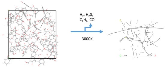
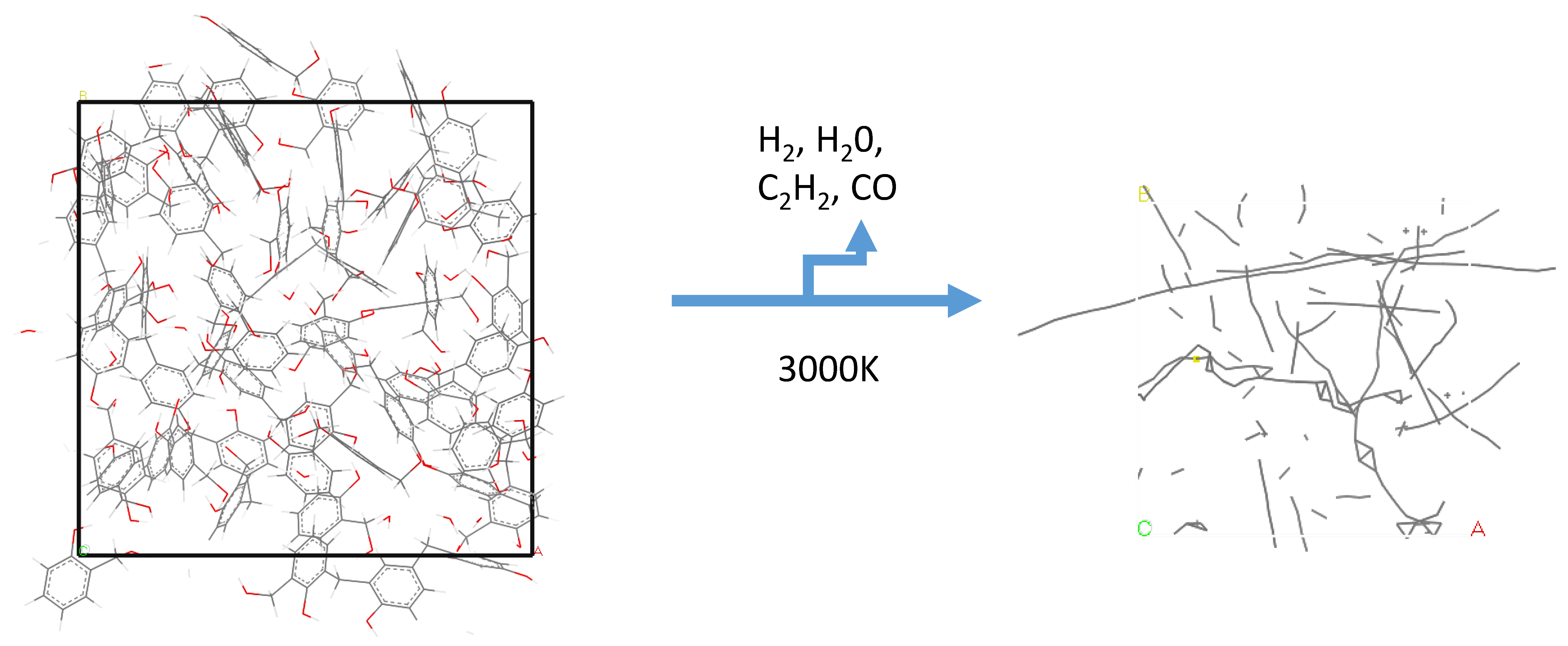
Without product removal, the model ran successfully for 1.5 ns, there was no graphitization observed and complete fragmentation occurred at 0.5 ns. With product removal and at a time step of 0.25 fs a carbon only system was achieved at 805 ps and at 1.5 ns long-chain carbon systems and cyclopropane rings were observed (Figure 5).
Figure 6 shows the array of disconnected atoms and groups at the end of the simulation, which is tending towards the glassy carbon char that is found experimentally.
4. Discussion
The thermal decomposition of polyphenolic resins was studied by reactive molecular dynamics (RMD) simulation at elevated temperatures. However, it should be noted that when multiple elementary reactions with different Arrhenius parameters are possible, the ratio of products is likely to be temperature-dependent. Atomistic models of the polyphenolic resins were constructed using an automatic method which calls routines from the software package Materials Studio. In order to perform some validation of the models, simulated densities and heat capacities were compared with experimental values. There are two molecular dynamics routines in the Materials Studio software and four options for thermostatic control, so these were compared. The most suitable combination for this system was the Forcite with the Nosé–Hoover thermostat, which gave values of heat capacity closest to the experimental values. Simulated densities approached a final density of 1.05–1.08 g/cm3 which compares favorably with experimental values of 1.16–1.21 g/cm3 for phenol-formaldehyde resins [36]. As some of our models were not 100% cured one would expect a lower density than experimental ones, and additionally, as many of our models are "wet”, i.e., water produced during the polymerization has not been removed, then the density would also be expected to be lower. Nevertheless, with only two models, 33% and 66% cured, a trend to increasing density was observed. None of the computed heat capacities agreed with the empirical value of 1.181–1.206 kJ·kg−1·K−1 at 298 K [35], although the longer simulations gave the closest values to the experimental ones, which were between 6 and 9 kJ·kg−1·K−1. The RMD calculations were run using the LAMMPS software, the ReaxFF force field, and an in-house routine for product removal. The species produced during RMD correlated with those found experimentally for polyphenolic systems and rearrangements to form cyclopropane moieties were observed. At the end of the RMD simulations a glassy carbon char resulted.
Supplementary Materials
The following are available online at https://www.mdpi.com/2504-477X/3/2/32/s1, Figure S1: (A) Model of 1000 atoms, 33% cured at 1250 K after 5 ps. (B) close up of (A), showing broken chains, (C) Model of 1000 atoms, 66% cured at 1250 K after 10 ps. (D) Model of 1000 atoms, 66% cured at 1250 K after 1.5 ns, showing cyclopropane rings.
Author Contributions
M.P., G.E., and S.H. carried out the work. All authors analysed the data and M.P. and B.H. wrote the paper.
Funding
The authors would like to thank the UK Ministry of Defence (MOD) for financial support for Stephen Hall and Grace Edmund, through MOD Centre for Defence Enterprise grant, contract number DSTLX1000089116.
Conflicts of Interest
The authors declare no conflict of interest.
References
- Stoliarov, S.; Nyden, M.; Lyon, R.E. Reactive dynamics model of thermal decomposition in polymers. In Proceedings of the 48th International SAMPE Symposium, Long Beach, CA, USA, 11–15 May 2003. [Google Scholar]
- Sanjukta, B.; Tamal, B.; Mohanty, K. Molecular dynamic simulation of spontaneous combustion and pyrolysis of brown coal using ReaxFF. FUEL 2014, 136, 326–333. [Google Scholar]
- Zhan, J.H.; Wu, R.; Liu, X.; Gao, S.; Xu, G. Preliminary understanding of initial reaction process for subbituminous coal pyrolysis with molecular dynamics simulation. FUEL 2014, 134, 283–292. [Google Scholar] [CrossRef]
- Castro-Marcano, F.; Russo Jr, M.F.; Van Duin, A.C.; Mathews, J.P. Pyrolysis of a large-scale molecular model for Illinois no. 6 coal using the ReaxFF reactive force field. J. Anal. Appl. Pyrolysis 2014, 109, 79–89. [Google Scholar] [CrossRef]
- Liu, X.; Li, X.; Liu, J.; Wang, Z.; Kong, B.; Gong, X.; Yang, X.; Lin, W.; Guo, L. Study of High Density polyethylene (HDPE) pyrolysis with reactive Molecular Dynamics. Polym. Degrad. Stab. 2014, 104, 62–70. [Google Scholar] [CrossRef]
- Liu, J.; Li, X.; Guo, L.; Zheng, M.; Han, J.; Yuan, X.; Nie, F.; Liu, X. Reaction analysis and visualization of ReaxFF molecular dynamics simulations. J. Mol. Graph. Model. 2014, 53, 13–22. [Google Scholar] [CrossRef]
- Chen, W.; Duan, H.T.; Hua, M.; Gu, K.L.; Shang, H.F.; Li, J. Comparison of Oxidation Resistance of UHMWPE and POM in H2O2 Solution from ReaxFF Reactive Molecular Dynamics Simulations. J. Phys. Chem. B 2014, 118, 10311–10318. [Google Scholar] [CrossRef]
- Zhou, T.; Liu, L.; Goddard, I.I.I.W.A.; Zybin, S.V.; Huang, F. ReaxFF reactive molecular dynamics on silicon pentaerythritol tetranitrate crystal validates the mechanism for the colossal sensitivity. Phys. Chem. Chem. Phys. 2014, 16, 23779–23791. [Google Scholar] [CrossRef] [Green Version]
- Zhou, T.; Song, H.; Liu, Y.; Huang, F. Shock initiated thermal and chemical responses of HMX crystal from ReaxFF molecular dynamics simulation. Phys. Chem. Chem. Phys. 2014, 16, 13914–13931. [Google Scholar] [CrossRef]
- Cheng, H.; Zhu, Y.A.; Chen, D.; Åstrand, P.O.; Li, P.; Qi, Z.; Zhou, X.G. Evolution of Carbon Nanofiber-Supported Pt Nanoparticles of Different Particle Sizes: A Molecular Dynamics Study. J. Phys. Chem. C 2014, 118, 23711–23722. [Google Scholar] [CrossRef] [Green Version]
- Zhang, C.; Wen, Y.; Xue, X. Self-Enhanced Catalytic Activities of Functionalized Graphene Sheets in the Combustion of Nitromethane: Molecular Dynamic Simulations by Molecular Reactive Force Field. ACS Appl. Mater. Interfaces 2014, 6, 12235–12244. [Google Scholar] [CrossRef]
- Li, G.Y.; Xie, Q.A.; Zhang, H.; Guo, R.; Wang, F.; Liang, Y.H. Pyrolysis Mechanism of Metal-Ion-Exchanged Lignite: A Combined Reactive Force Field and Density Functional Theory Study. Energy Fuels 2014, 28, 5373–5381. [Google Scholar] [CrossRef]
- Zhang, B.; van Duin, A.C.T.; Johnson, J.K. Development of a ReaxFF Reactive Force Field for Tetrabutylphosphonium Glycinate/CO2 Mixtures. J. Phys. Chem. B 2014, 118, 12008–12016. [Google Scholar] [CrossRef]
- Fantauzzi, D.; Bandlow, J.; Sabo, L.; Mueller, J.E.; van Duin, A.C.; Jacob, T. Development of a ReaxFF potential for Pt-O systems describing the energetics and dynamics of Pt-oxide formation. Phys. Chem. Chem. Phys. 2014, 16, 23118–23133. [Google Scholar] [CrossRef]
- Schönfelder, T.; Friedrich, J.; Prehl, J.; Seeger, S.; Spange, S.; Hoffmann, K.H. Reactive force field for electrophilic substitution at an aromatic system in twin polymerization. Chem. Phys. 2014, 440, 119–126. [Google Scholar] [CrossRef]
- Cheng, T.; Jaramillo-Botero, A.; Goddard, I.I.I.W.A.; Sun, H. Adaptive Accelerated ReaxFF Reactive Dynamics with Validation from Simulating Hydrogen Combustion. J. Am. Chem. Soc. 2014, 136, 13467. [Google Scholar] [CrossRef]
- Kylasa, S.B.; Aktulga, H.M.; Grama, A.Y. PuReMD-GPU: A reactive molecular dynamics simulation package for GPUs. J. Comput. Phys. 2014, 272, 343–359. [Google Scholar] [CrossRef]
- Farah, K.; Muller-Plathe, F.; Bohm, M.C. Classical Reactive Molecular Dynamics Implementations: State of the Art. Minireview. ChemPhysChem 2012, 13, 1127–1151. [Google Scholar] [CrossRef]
- Xiao, H.; Shi, X.; Hao, F.; Liao, X.; Zhang, Y.; Chen, Y. Development of a Transferable Reactive Force Field of P/H Systems: Application to the Chemical and Mechanical Properties of Phosphorene. J. Phys. Chem. A 2017, 121, 6135–6149. [Google Scholar] [CrossRef] [Green Version]
- Gardziella, A.; Knop, A.; Pilato, L.A. Phenolic Resins, 2nd ed.; Springer: Berlin, Germany, 2000; pp. 83–90. [Google Scholar]
- Fakirov, S. Fundamentals of Polymer Science for Engineers; Wiley-VCH: Weinheim, Germany, 2017. [Google Scholar]
- Hall, S.A.; Howlin, B.J.; Hamerton, I.; Baidak, A.; Billaud, C.; Ward, S. Solving the Problem of Building Models of Crosslinked Polymers: An Example Focussing on Validation of the Properties of Crosslinked Epoxy Resins. PloS ONE 2012. [Google Scholar] [CrossRef]
- Jensen, F. Introduction to Computational Chemistry, 2nd ed.; Wiley: Chichester, UK, 2007; pp. 445–471. [Google Scholar]
- Woodcock, L.V. Isothermal molecular dynamics calculations for liquid salts. Chem. Phys. Lett. 1971, 10, 257–261. [Google Scholar] [CrossRef]
- Hünenberger, P.H. Thermostat Algorithms for Molecular Dynamics Simulations. Adv. Polym. Sci. 2005, 173, 105–149. [Google Scholar]
- Andersen, H.C.J. Molecular dynamics simulations at constant pressure and/or temperature. Chem. Phys. 1980, 72, 2384–2393. [Google Scholar] [CrossRef]
- Berendsen, H.J.C.; Postma, J.P.M.; van Gunsteren, W.F.; DiNola, A.; Haak, J.R. Molecular dynamics with coupling to an external bath. J. Chem. Phys. 1984, 81, 3684–3690. [Google Scholar] [CrossRef]
- Morishita, T.J. Fluctuation formulas in molecular-dynamics simulations with the weak coupling heat bath. Chem. Phys. 2000, 113, 2976–2982. [Google Scholar] [CrossRef]
- Nosé, S. A molecular dynamics method for simulations in the canonical ensemble. Mol. Phys. 1984, 52, 255–268. [Google Scholar] [CrossRef]
- Nosé, S.J. A unified formulation of the constant temperature molecular dynamics methods. Chem. Phys. 1984, 81, 511–519. [Google Scholar]
- Hoover, W.G. Canonical dynamics: Equilibrium phase-space distributions. Phys. Rev. A 1985, 31, 1695–1697. [Google Scholar] [CrossRef]
- Allen, M.P.; Tildesley, D.J. Computer Simulation of Liquids; Oxford University Press: New York, NY, USA, 1989. [Google Scholar]
- McNaught, A.D.; Wilkinson, A. Compendium of Chemical Terminology, 2nd ed.; Blackwell Scientific Publications: Oxford, UK, 1997. [Google Scholar]
- Fyfe, C.A.; McKinnon, A.R.; Tchir, W.J. Investigation of the Mechanism of the Thermal Decomposition of Cured Phenolic Resins by High-Resolution 13C CP/MAS Solid-state NMR Spectroscopy. Macromolecules 1983, 16, 1216–1219. [Google Scholar] [CrossRef]
- Erä, V.A.; Mattila, A.; Lindberg, J. Determination of specific heat of phenol formaldehyde resol resins by differential scanning calorimetry. J. Angew. Makromol. Chem. 1977, 64, 235–238. [Google Scholar] [CrossRef]
- Trick, K.A.; Saliba, T.E. Mechanisms of the pyrolysis of phenolic resin in a carbon/phenolic composite. Carbon 1995, 33, 1509–1515. [Google Scholar] [CrossRef]
Figure 1.
Scheme for the formation of polyphenolic resins.

Figure 2.
(A) Model of 1000 atoms, 33% cured and temperature cycle data for 1000 atoms, 33% cured. (B) Model of 1000 atoms, 66% cured and temperature cycle data for 1000 atoms, 66% cured.
Figure 2.
(A) Model of 1000 atoms, 33% cured and temperature cycle data for 1000 atoms, 33% cured. (B) Model of 1000 atoms, 66% cured and temperature cycle data for 1000 atoms, 66% cured.

Figure 3.
Convergence of energies in the model under conventional molecular dynamics simulation. Figure 2A (left) and Figure 2B (right): Variation in energy across a 200 ps RMD simulation of the 1000 atom, 100% cured phenol-formaldehyde resin (PFR) model generated by Forcite (Left) and Discover (Right).
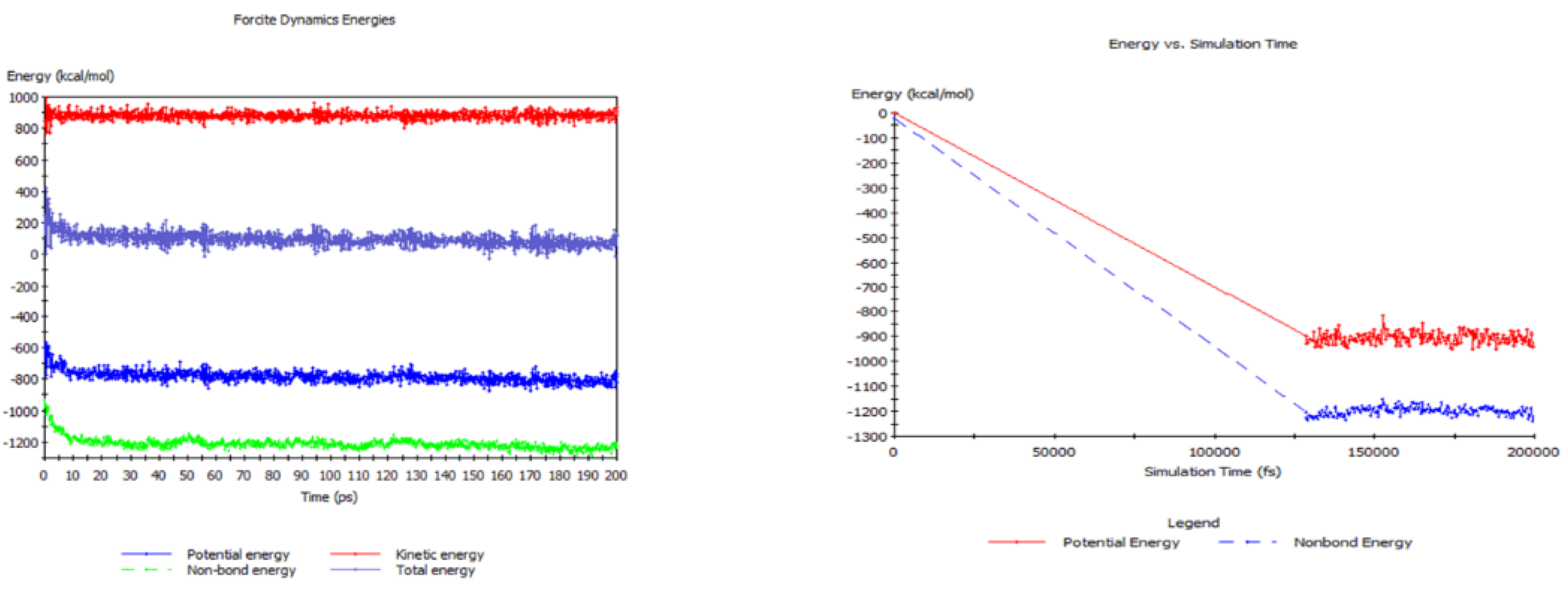
Figure 4.
Evolution of small molecule species versus RMD simulation time.
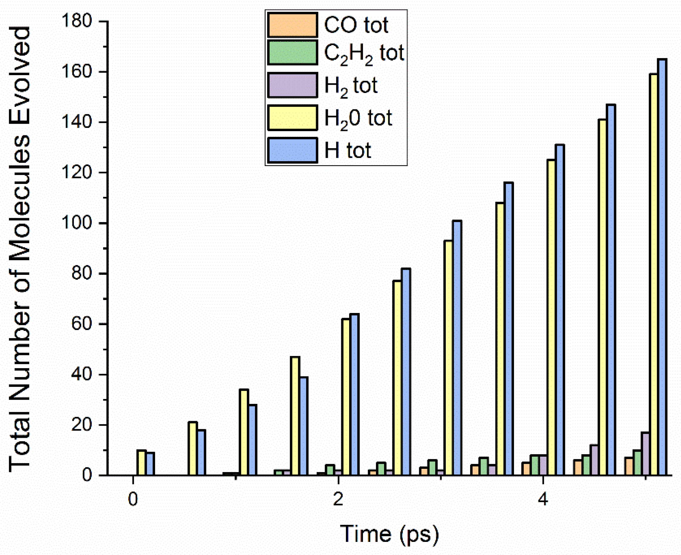
Figure 5.
(A) Model of 1000 atoms, 100% cured (wet). (B) Model of 1000 atoms, 100% cured after 5 ps RMD simulation at 1250 K.
Figure 5.
(A) Model of 1000 atoms, 100% cured (wet). (B) Model of 1000 atoms, 100% cured after 5 ps RMD simulation at 1250 K.

Figure 6.
Model of 1000 atoms, 100% cured at 1250 K after 1.5 ns.


Table 1.
Average temperature and standard deviation of total energy retrieved from the reactive molecular dynamics (RMD) simulations of each of the models using the Nosé–Hoover thermostat in the Discover module.
Table 1.
Average temperature and standard deviation of total energy retrieved from the reactive molecular dynamics (RMD) simulations of each of the models using the Nosé–Hoover thermostat in the Discover module.
| tsim (ps) | Cure % of 1000 Atom Model | Forcite | Discover | ||
|---|---|---|---|---|---|
| Tavg (K) | E (kJ·mol−1) | Tavg (K) | E (kJ·mol−1) | ||
| 5 | 33% Cured | 299.728 | 843 | 277.924 | 617 |
| 50 | 33% Cured | 300.002 | 318 | 275.732 | 257 |
| 200 | 33% Cured | 299.997 | 229 | 276.660 | 183 |
| 5 | 66% Cured | 299.714 | 707 | 277.059 | 661 |
| 50 | 66% Cured | 300.014 | 310 | 276.983 | 277 |
| 200 | 66% Cured | 300.004 | 245 | 276.000 | 186 |
| 5 | 100% Cured | 297.883 | 632 | 276.527 | 677 |
| 50 | 100% Cured | 300.001 | 285 | 277.012 | 272 |
| 200 | 100% Cured | 300.005 | 196 | 275.565 | 186 |
Table 2.
Computed values of the heat capacity per atom (Cv/N) and specific heat capacity (S) for the 48 RMD simulations of each of the models using the Nosé–Hoover thermostat in Discover and Forcite over 5, 50, and 200 ps.
Table 2.
Computed values of the heat capacity per atom (Cv/N) and specific heat capacity (S) for the 48 RMD simulations of each of the models using the Nosé–Hoover thermostat in Discover and Forcite over 5, 50, and 200 ps.
| tsim (ps) | Cure % of 1000 Atom Model | Forcite | Discover | ||
|---|---|---|---|---|---|
| Cv/N (J·mol−1·K−1) | S (kJ·kg−1·K−1) | Cv/N (J·mol−1·K−1) | S (kJ·kg−1·K−1) | ||
| 5 | 33% Cure | 951.496 | 125.525 | 592.973 | 78.227 |
| 50 | 33% Cure | 135.554 | 17.883 | 104.376 | 13.770 |
| 200 | 33% Cure | 70.386 | 9.286 | 52.864 | 6.974 |
| 5 | 66% Cure | 670.403 | 88.442 | 685.086 | 90.379 |
| 50 | 66% Cure | 128.226 | 16.916 | 120.336 | 15.875 |
| 200 | 66% Cure | 80.072 | 10.563 | 54.822 | 7.232 |
| 5 | 100% Cure | 541.234 | 71.402 | 721.952 | 95.243 |
| 50 | 100% Cure | 108.441 | 14.306 | 116.422 | 15.359 |
| 200 | 100% Cure | 51.573 | 6.804 | 54.924 | 7.246 |
Table 3.
Small molecule species produced by temperature region (from Trick and Saliba).
| Region 1 (573–823 K) | Region 2 (673–1073 K) | Region 3 (833–1173 K) | |||
|---|---|---|---|---|---|
| Species | Molar % | Species | Molar % | Species | Molar % |
| H | 0 | H | 59.4 | H | 0 |
| H2 | 0 | H2 | 0 | H2 | 85.7 |
| H2O | 49.8 | H2O2 | 12.7 | H2O | 4.70 |
| CO | 0 | CO | 12.7 | CO | 9.5 |
| O2 | 0.1 | O2 | 0 | O2 | 0 |
| CO2 | 0 | CO2 | 0.2 | CO2 | 0.1 |
| CH4 | 0 | CH4 | 14.9 | CH4 | 0 |
| C2H6 | 0 | C2H6 | 0.1 | C2H6 | 0 |
| Phenol, Cresol | 50.1 | Phenol, Cresol | 0 | Phenol, Cresol | 0 |
© 2019 by the authors. Licensee MDPI, Basel, Switzerland. This article is an open access article distributed under the terms and conditions of the Creative Commons Attribution (CC BY) license (http://creativecommons.org/licenses/by/4.0/).
Share and Cite
MDPI and ACS Style
Purse, M.; Edmund, G.; Hall, S.; Howlin, B.; Hamerton, I.; Till, S. Reactive Molecular Dynamics Study of the Thermal Decomposition of Phenolic Resins. J. Compos. Sci. 2019, 3, 32. https://doi.org/10.3390/jcs3020032
AMA Style
Purse M, Edmund G, Hall S, Howlin B, Hamerton I, Till S. Reactive Molecular Dynamics Study of the Thermal Decomposition of Phenolic Resins. Journal of Composites Science. 2019; 3(2):32. https://doi.org/10.3390/jcs3020032
Chicago/Turabian StylePurse, Marcus, Grace Edmund, Stephen Hall, Brendan Howlin, Ian Hamerton, and Stephen Till. 2019. "Reactive Molecular Dynamics Study of the Thermal Decomposition of Phenolic Resins" Journal of Composites Science 3, no. 2: 32. https://doi.org/10.3390/jcs3020032