Durability of Composite Materials under Severe Temperature Conditions: Influence of Moisture Content and Prediction of Thermo-Mechanical Properties During a Fire

Abstract

The main objective of the present study was to develop a fire thermal model able to predict the evolution of the temperature and decomposition gradient across a laminated composite structure when exposed to fire. The thermal response of composite laminate made of organic polymer matrix was investigated under severe temperature conditions as samples were exposed to high temperatures up to 750 °C. The highlight is that a behavior law for water is included in our thermo-mechanical model to estimate effects due to a moisture content field on the thermal response of composite laminates. In particular, porosity and gas pressure are strongly influenced by the presence of water in the material and modify the thermal behavior accordingly. This enabled us to propose a new approach that can be used for the prediction of hygro-thermo-chemico-mechanical post-combustion properties in a very large number of material and fire scenarios.

1. Introduction

Analyses under extreme conditions make it possible to put a material in non-ambient conditions. The properties of that material are often drastically modified and new properties can then be studied. These properties could change when a material is subjected to severe environmental conditions of low or high temperatures [1,2], often coupled to a second stress such as an intense magnetic field, a light irradiation [3,4], a mechanical stress [5,6], or a high pressure [7,8]. Under these extreme conditions, the studied material undergoes important physical and/or chemical modifications, often leading to the appearance of phase transitions [9,10] or metastable states. It is then very challenging to understand the behavior of materials under extreme conditions in order to predict and optimize their properties under normal conditions of pressure and temperature, thus allowing their use for new sensors having piezo- or thermo-chromic applications, for instance. Measurements in extreme conditions are both a scientific challenge, to understand the properties of materials, and a technical challenge to study the material in specific and very severe environments. The field of composite materials with organic matrix does not escape this trend [11] and, in this work, we focus on the analysis of the hygro-thermo-chemico-mechanical properties of laminated composite materials (organic polymer matrixes such as vinylester, polyester, or phenolic, with ceramic reinforcements such as E-glass or carbon fibers) in the case of fire resistance, i.e., in high temperature conditions and in the presence of an initial moisture content field.

The use of composite materials has grown exceptionally in the last forty years, substituting traditional engineering materials, such as steels and aluminum alloys, in many industries. This is particularly true in the marine, aircraft, aerospace, and car industries. For certain applications, their properties exceed those of metallic materials, in particular by their high strength-to-weight ratio. Laminated composite materials can present some disadvantages, such as a moderate resistance to heat, mechanical load, or hygroscopic aging, which will be more or less important depending on the choice of the constituents (matrix and reinforcement) of the composite laminate. As a consequence, mechanical properties of composite laminates are susceptible to be reduced in extreme conditions. As a result, the use of this type of composite materials must be done with care, especially in situations that involve risk of damage due to fire [12]. Because of this, a better understanding of the phenomena providing improved fire resistance of laminated composite materials is mandatory for designing safer structures.

In this study, we focused our work on the description and evaluation of a hygro-thermal model capable of estimating the thermal degradation as well as the evolution of the temperature through the thickness of composite laminates with organic polymer matrixes and ceramic reinforcements with the internal presence of water. It will enable us to formulate another model for the computation of the mechanical properties and post-combustion of laminated composite materials, which will be useful to predict the durability of composite laminates exposed to extreme conditions of temperature and humidity (i.e., accounting for the presence of an initial moisture content field).

2. Materials and Methods

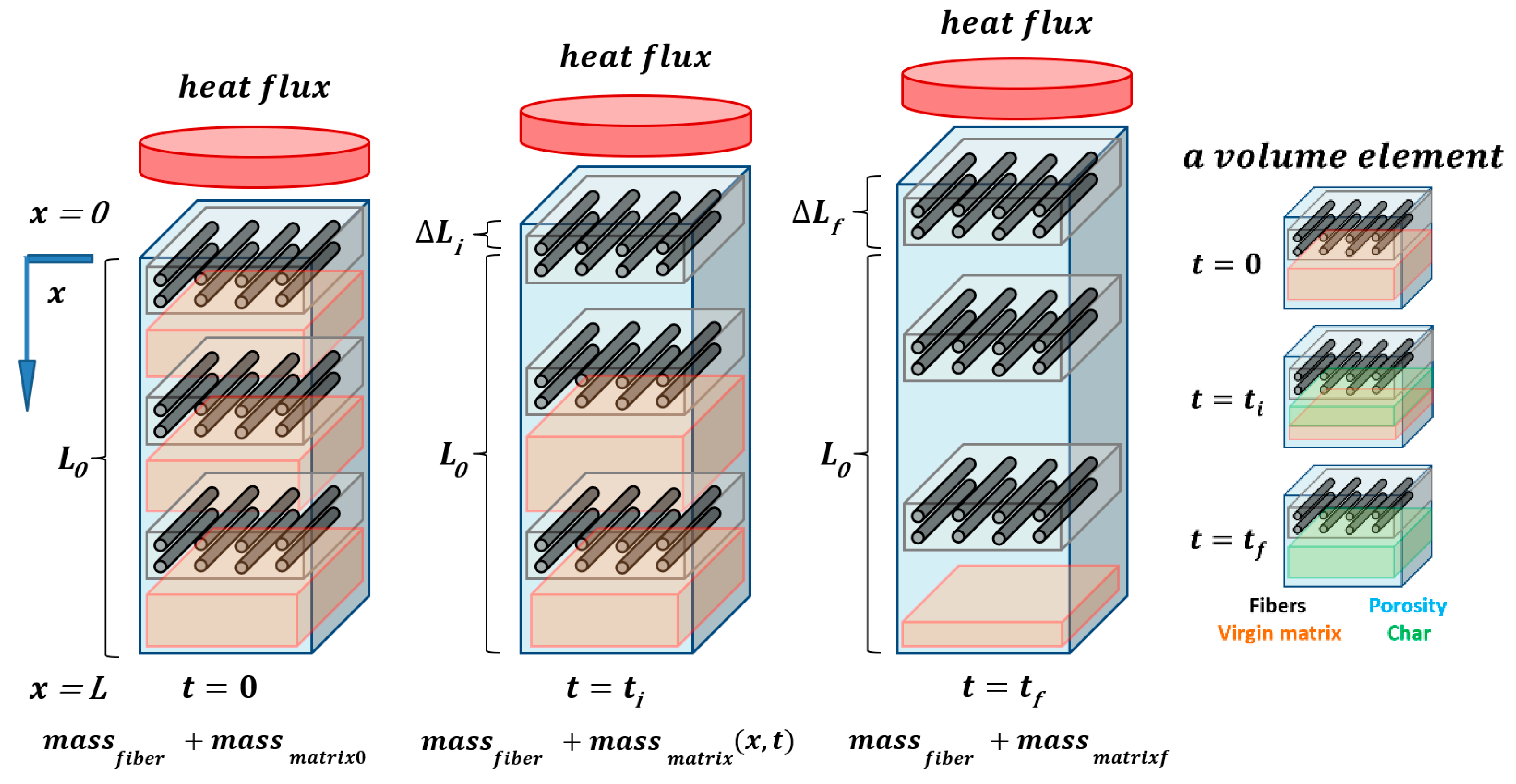
2.1. Thermal Model Development

The thermal model that we propose lets us obtain the mass loss produced due to the polymer matrix decomposition and the temperature field through the thickness of laminated composite materials exposed to fire. Most of the models in the literature are developed on this principle. Our model is based on other quantities of interest, such as the thermal expansion, the porosity, the permeability, the stocked gases mass, and the internal pressure, which are not usually modeled or not evaluated in common models proposed by other authors [13,14]. The mathematical model is developed for the case of unidirectional heat transfer in a polymer composite laminate and is based on the work published by Henderson and Wiecek [15]. Certain assumptions must be introduced to simplify this model: Thermal exchanges between the decomposition gases and the solid material occur until thermal equilibrium; moreover, a decoupling of the composite fire is considered, which means the flame itself is not modeled. The latter is represented as a constant heat flux which is not modified by the thermal degradation of the material. The initiation and development of fire are not taken into account in the analysis. Moreover, the behavior of the decomposition gases is assumed to be ideal. The gas flow will be governed by Darcy’s law and the absence of reaction of the decomposition gases is supposed.

Our model expresses the heat transfer and analyzes the three most influential energy transfer processes that take place during the degradation of a composite exposed to fire that are susceptible to significantly affect the temperature field through the material thickness. It also considers a thermo-chemical expansion produced only on the heat flux direction. These processes are the conductive heat transfer through the composite laminate, the heat production or consumption by the decomposition reaction of the polymer matrix, and the convective mass transfer of volatile products from the decomposed regions to the hot composite surface. The one-dimensional energy conservation equation that we propose is expressed by:

$$\begin{array}{c}[m_s(x,t)c_p(x,t)+m_g(x,t)c_{pg}(x,t)]\frac{\partial T(x,t)}{\partial t}=\frac{\partial }{\partial x}\{[k_g(x,t)\varphi (x,t)+k_x(x,t)(1-\\ \varphi (x,t))]\frac{\partial T(x,t)}{\partial x}\}\Delta x(x,t)\Delta A-{\dot{m}}_g(x,t)c_{pg}(x,t)\frac{\partial T(x,t)}{\partial x}\Delta x(x,t)+\\ m_s(x,t) A {[\alpha (x,t)]}^n{e}^{-\frac{E_a}{R T(x,t)}}[Q_p+h_s(x,t)-h_g(x,t)].\end{array}$$

(1)

With the heat Equation (1) mentioned above, we explain the thermal behavior through thickness of laminated composite materials exposed to a constant unidirectional heat flux. The first term of the right member of Equation (1) represents the induced effect on temperature T(x, t) by heat conduction through the thickness of the solid material $k_x\left(x,t\right)$ and the gases $k_g\left(x,t\right)$, as well as that due to the influence of the transverse thermal conductivity transformation by increasing the temperature. The second term corresponds to the convection of the volatile species: The internal convection of the thermal energy due to the transport of decomposition gases ${\dot{m}}_g\left(x,t\right)$, which heats up by flowing toward the surface exposed to fire. The last term describes the change in temperature due to the generation or to the heat consumption resulting from the decomposition of the resin. This term is negative when the decomposition process is endothermic and positive when it is exothermic. These terms are influenced by the increase of the internal pressure through the porosity $\varphi \left(x,t\right)$, as well as the thermal expansion through the variable $\Delta x\left(x,t\right),$ which represent the instantaneous expansion/contraction of solid matrix having a thickness $L\left(x,t\right)$, with respect to the initial thickness $L_0$ of the sample. In Equation (1), T(x, t) is the instantaneous temperature at a considered point of interest, where t and x are the time and the through-thickness coordinate respectively, placed through the direction of the thickness at the distance x from the front surface. The parameters $m_s\left(x,t\right)$, $m_g\left(x,t\right)$, $c_p\left(x,t\right)$,$c_{pg}\left(x,t\right)$, $k_x\left(x,t\right)$, and $k_g\left(x,t\right)$ are the solid laminate and gases mass, specific heat of solid laminate and gases, and the thermal conductivity of the solid composite and gases in the direction of thickness. $Q_p$ is the endothermic decomposition energy of the polymer matrix. The term ${\dot{m}}_g\left(x,t\right)$ is the mass flow of the volatile products. The terms $h_s\left(x,t\right)$ and $h_g\left(x,t\right)$ are the enthalpies of the solid laminated composite material and volatiles, respectively, expressed as follows:

$$h_s\left(x,t\right)={{\displaystyle \int }}_{T_{\infty }}^{T\left(x,t\right)}{c}_p\left(x,t\right) dT,$$

(2)

$$h_g\left(x,t\right)={{\displaystyle \int }}_{T_{\infty }}^{T\left(x,t\right)}{c}_{pg}\left(x,t\right) dT,$$

(3)

with $T_{\infty }$ referring to the ambient temperature.

In the present work, a modification of Equation (1) is proposed in order to account for the mass loss rate of the polymer matrix directly in the last term of Equation (1), similarly to what is proposed by Gibson et al. [14], who proposed to express the material decomposition rate $\left(\frac{\partial m\left(x,t\right)}{\partial t}\right)$ in their known thermal model. In the following, the mass decomposition of the resin will be assumed to satisfy a typical Arrhenius law:

$$\frac{1}{m_{m0}-m_{mf}}\frac{\partial m_m\left(x,t\right)}{\partial t}=-A {\left[\alpha \left(x,t\right)\right]}^n{e}^{-\frac{E_a}{R T\left(x,t\right)}},$$

(4)

where $A$, $E_a$, and $n$ are the reaction rate constant, the activation energy of the decomposition reaction, and the reaction order, respectively. All of these quantities can be determined in practice owing to the thermo-gravimetric analysis (TGA) of the polymer matrix. Certain polymer degradation kinetics must be modeled by several steps due to different reactions happening during the thermal degradation. Moreover, the application of a high heat flux also impose the modeling of fiber degradation. These aspects can be included in the model, expanding Equation (2) in the appropriate number of steps related to the numbers of material degradation reactions.

In Equation (1) and Equation (4) mentioned above, $\alpha \left(x,t\right)$ represents the fraction of virgin material remaining in the solid matrix:

$$\alpha \left(x,t\right)=\frac{m_m\left(x,t\right)-m_{mf}}{m_{m0}-m_{mf}},$$

(5)

where $m_m\left(x,t\right)$, $m_{m0}$, and $m_{mf}$ are the instantaneous, initial, and final masses of the polymer matrix, respectively, which are experimentally determined analyzing the TGA curve of resin decomposition. The term $\alpha \left(x,t\right)$ is used as a local variable to account for the advancement of the decomposition process. It will make it possible to distinguish between the instantaneous fraction of the virgin material and the remaining material (i.e., char material) which appears during the decomposition of the material.

In addition, another partial differential equation must be formulated for the through-thickness thermal expansion [16]:

$$\frac{1}{L_0}\frac{\partial L\left(x,t\right)}{\partial t}={\alpha }_v \alpha \left(x,t\right)\frac{\partial T\left(x,t\right)}{\partial t}+{\alpha }_c\left[1-\alpha \left(x,t\right)\right]\frac{\partial T\left(x,t\right)}{\partial t}+\frac{\eta }{m_{m0}}\frac{\partial m_m\left(x,t\right)}{\partial t},$$

(6)

with ${\alpha }_v$ and ${\alpha }_c$ referring to linear expansion coefficient of virgin and char materials, respectively. $\eta$ is the non-dimensional expansion factor resulting from the pyrolytic decomposition of a solid matrix. Equation (6) allows us to define the thermal through-thickness expansion profiles (fraction length change, (FLC)) as shown in the following.

A similar partial differential equation let us model the variation of material permeability [15]:

$$\frac{1}{{\gamma }_0}\frac{\partial \gamma \left(x,t\right)}{\partial t}={\psi }_v \alpha \left(x,t\right)\frac{\partial T\left(x,t\right)}{\partial t}+{\psi }_c\left[1-\alpha \left(x,t\right)\right]\frac{\partial T\left(x,t\right)}{\partial t}+\frac{\zeta }{m_{m0}}\frac{\partial m_m\left(x,t\right)}{\partial t},$$

(7)

where $\gamma \left(x,t\right)$ is the instantaneous permeability of a material element located in the thickness at coordinate x, ${\gamma }_0$ is the initial permeability, ${\psi }_v$ and ${\psi }_c$ represent the permeability coefficient of virgin and char materials, respectively, and $\zeta$ is the non-dimensional permeability factor introduced in order to account for the contribution resulting from the pyrolytic decomposition of solid matrix.

The gas storage in the solid matrix and the gas mass flux are calculated by the mass conservation equation, which is simplified as follows [17]:

$$-\frac{\partial m_s\left(x,t\right)}{\partial t}=\frac{\partial m_g\left(x,t\right)}{\partial t}+\frac{\partial {\dot{m}}_g\left(x,t\right)}{\partial t}\Delta x\left(x,t\right).$$

(8)

In Equation (8), the transport phenomena of decomposition gas through the material thickness is related to the decomposition rate, which is assumed to follow a typical Arrhenius expression (Equation (4)).

Thanks to the assumptions on the ideal behavior of the decomposition gases and the gas flow governed by Darcy’s law, the transport velocity of the gases mass flow, ${\dot{m}}_g\left(x,t\right)$, can be expressed using Darcy’s equation:

$${\dot{m}}_g\left(x,t\right)=-\frac{\gamma \left(x,t\right) m_g\left(x,t\right)}{\mu \varphi \left(x,t\right) \Delta x\left(x,t\right)}\frac{\partial P\left(x,t\right)}{\partial x},$$

(9)

where $\mu$ stands for the viscosity of decomposition gases.

The pressure $P\left(x,t\right)$ is defined by the ideal gas state equation, modified as follows by the material porosity:

$$P\left(x,t\right)=-\frac{m_g\left(x,t\right) R T\left(x,t\right)}{M \varphi \left(x,t\right) \Delta x\left(x,t\right)},$$

(10)

where R is the ideal gas constant and M is the average molecular weight of decomposition gases.

The influence of the pressure due to the gas storage in the material is still implicitly taken into account in the equation of heat (Equation (1)), whose term of conductivity heat transfer is modified by the porosity. Equation (1) is also coupled with the thermal expansion equation, which is due in part to these pressure changes. Figure 1 represents a scheme of the thermal degradation of composite materials considering thermal expansion. The idea is to discretize the thickness of the material in n elements, for example three elements in the case of Figure 1. Each element consists of an amount of fibers (black cylinder), an amount of matrix (orange), and an amount of air porosity (blue). This constitutes 100% of one element, with the proportions changing as the combustion time increases. It is thus noted that at t_f, the first element contains only fibers and a greater porosity, the medium element is in the same state of degradation, and finally that the lower element always contains the same amount of fibers (because they do not decompose at this temperature) and that it still contains a little matrix quantity while the amount of porosity has increased. This schematization makes it possible to have a close look at the thermal behavior in every through-thickness position of the material.

We note $\Delta x\left(x,t\right),$ the variable control cell during decomposition of the resin matrix. First, the material is supposed to consist of different elements in the through-thickness direction x and in each element there is a mass of fibers and a mass of polymer matrix. Over time, the polymer matrix begins to decompose with the release of volatile substances and a loss of matrix mass progressively evolves through the thickness, according to Equation (4). At the end, the entire matrix degrades, leaving a char residue and fibers. One has to note that fibers in the present study are assumed not to decompose due to the considered heat flux. This modeling makes it possible to evaluate local quantities, at each through-thickness coordinate x and over time, based on certain global quantities, such as the initial and final mass of the matrix, the fibers mass, and the initial and final matrix volume fractions before and after its decomposition.

Following the presented modeling, thermal properties of partially degraded composite material are modeled using homogenization laws, because information on the progress of the pyrolysis reaction is not easily available with current means. Then, the conductivity and specific heat of composite material during decomposition can be modeled through mixture laws between the virgin and char states of the composite material [15]:

$$k_x\left(x,t\right)=\alpha \left(x,t\right) k_v\left(T\left(x,t\right)\right)+\left[1-\alpha \left(x,t\right)\right] k_c\left(T\left(x,t\right)\right),$$

(11)

$$c_p\left(x,t\right)=\alpha \left(x,t\right) c_{pv}\left(T\left(x,t\right)\right)+\left[1-\alpha \left(x,t\right)\right] c_{pc}\left(T\left(x,t\right)\right),$$

(12)

where $k_v\left(T\right)$, $c_{pv}\left(T\right)$, $k_c\left(T\right)$, and $c_{pc}\left(T\right)$ are the thermal conductivity and specific heat of virgin and char materials, respectively. These thermal properties can be determined experimentally as a function of temperature for the analyzed composite material before the start of decomposition and after carbonization.

Mixture laws let us estimate values of the effective macroscopic thermal behavior of composite materials from the knowledge of local quantities. It is possible to model thermal properties as a function of time and through-thickness coordinate according to mean field approaches, considering the progress of decomposition reaction through the parameter $\alpha \left(x,t\right)$.

Initial and boundary conditions must be established to make it possible to numerically solve the thermal problem. Initial conditions involve all unknowns of the problem:

$$T\left(x,0\right)=T_{\infty },\hspace{1em}{m}_m\left(x,0\right)=m_{m0},\hspace{1em}{\dot{m}}_g\left(x,0\right)=0\hspace{1em}\mathrm{for} 0\le x\le L,$$

(13)

$$m_g\left(x,0\right)=m_{g0},\hspace{1em}P\left(x,0\right)=P_0,\hspace{1em}L\left(x,0\right)=L_0\hspace{1em}\mathrm{for} 0\le x\le L.$$

(14)

The heat transfer from the heating source to the composite during exposure to fire is the result of a thermal interaction between the frontal hot surface of the composite sample and the source itself. When the heating source is represented by fire, the heat is transferred mainly by radiative mechanisms [17]. The energy balance at the hot surface $\left(x=0\right)$ of the composite sample is described by the Stefan–Boltzmann law, considering also the thermal convection of the heating source:

$$\begin{gathered} -\left[k_g\left(x,t\right)\varphi \left(x,t\right)+k_x\left(x,t\right)\left(1-\varphi \left(x,t\right)\right)\right]{\frac{\partial T\left(x,t\right)}{\partial x}|}_{x=0} \\ =\left[{\epsilon }_s q_{radiation}^{″}-\sigma {\epsilon }_{msup}{T}^4\left(x,t\right)\right]+h_{convsup}\left[T_{\infty }-T\left(x,t\right)\right] \\ \mathrm{for} x=0 \mathrm{and} \forall t>0 \end{gathered}$$

(15)

In Equation (15), the right-hand term represents the net surface heat flux received by the frontal surface of the composite [18]. The net surface heat flux is the combination of the radiative and convective contributions. ${\epsilon }_s$ is the emissivity of the source, ${\epsilon }_{msup}$ is the emissivity of the front surface of the composite, and $h_{convsup}$ is the convection coefficient in the front surface of the composite. $\sigma$ is Stefan–Boltzmann’s constant.

The boundary condition on the face of the composite not being exposed to the heat source $\left(x=L\right)$ is also written as the sum of radiative and convective contributions:

$$\begin{gathered} -\left[k_g\left(x,t\right)\varphi \left(x,t\right)+k_x\left(x,t\right)\left(1-\varphi \left(x,t\right)\right)\right]{\frac{\partial T\left(x,t\right)}{\partial x}|}_{x=L} \\ =\sigma {\epsilon }_{minf}\left[T^4\left(x,t\right)-T_{\infty }^4\right]+h_{convinf}\left[T\left(x,t\right)-T_{\infty }\right] \\ \mathrm{for} x=L \mathrm{and} \forall t>0, \end{gathered}$$

(16)

where ${\epsilon }_{minf}$ and $h_{convinf}$ refer to the emissivity and convection coefficients of heat in the back surface of the composite material. The emissivity and the convection coefficients are different for the hot and the cold surfaces. These parameters can be functions of temperature $T\left(x,t\right)$ and the degree of decomposition $\alpha \left(x,t\right)$. However, these variations are quite small, thus both coefficients are often considered as constant values for each of the two surfaces, with the cold surface being characterized by lower values of these quantities resulting from the partial thermal insulation of the back surface (supposedly diffuse, grey, and opaque), which is typically used in order to achieve experimental tests of thermal degradation of composites.

The boundary conditions expressed by Equation (15) and Equation (16) are implicitly influenced by internal pressure rise through the volume fraction of porosity $\varphi \left(x,t\right)$.

Other boundary conditions on the back surface $\left(x=L\right)$ involving the mass flow of gases ${\dot{m}}_g\left(x,t\right)$ and the internal pressure $P\left(x,t\right)$ are necessary to close the thermal problem:

$${\dot{m}}_g\left(L,t\right)=0, P\left(L,t\right)=P_0 \mathrm{for} x=L \mathrm{and} \forall t>0.$$

(17)

The thermo-chemical degradation problem for composite materials is well defined by Equations (1), (4), (6)–(10) with initial and boundary conditions (Equations (13)–(17)). All variables involved in their formulation, which represent the unknowns of the problem, are instantaneous local quantities during the time of exposure to fire, i.e., they are functions of both the abscissa x and time t. They are all coupled with each other. Thus, the problem is mathematically represented by a non-linear system of partial differential equations (PDEs), with variable source terms and boundary conditions (in time and in space) that must be solved numerically for each step of time and through-thickness coordinate and simultaneously for the mass, the temperature, the transport velocity of the gases, the thermal expansion, the gas storage, the pressure, and the permeability, due to the complexity of the coupling of all the variables involved.

A numerical method was implemented in Mathematica 10, using the command NDSolve in order to solve the problem by the finite difference method [19]. This command uses the method of lines to solve partial differential equations by discretizing along the thickness direction, then by integrating the semi-discrete problem as a system of ordinary differential equations (ODEs) or a system of differential algebraic equations (DAEs). It is necessary that the PDEs problem is well posed as an initial value problem (Cauchy) in at least one dimension, since the ODE and DAE integrators used are solvers of initial value problems. The thermal problem verifies this condition, with initial Dirichlet conditions $\left(t=0\right)$ and with Neumann boundary conditions $\left(x=0\right)$ and $\left(x=L\right)$, expressed as a function of the temperature $T\left(x,t\right)$ and its derivative with respect to $\left(\frac{\partial T\left(x,t\right)}{\partial x}\right)$. The resolution of the PDE system follows a scheme of explicit differences, where the spatial variables are represented by central differences, since conditions are imposed at the limits of the x-coordinate, while the terms derived from time are represented by direct differences due to the fixed initial conditions at time t = 0. This numerical method provides interpolation functions as the results to unknowns, in order to evaluate them as a function of time and through-thickness coordinate.

2.2. Post-Combustion Mechanical Response

Post-combustion properties enable us to evaluate the decrease of the residual mechanical properties of the material after a certain time of exposure to fire, once the fire is extinguished after this time, and when the material reaches the ambient temperature. These properties are used to evaluate the residual mechanical integrity and safety of the structure where the material is used. It can be experimentally measured by three-point bending flexural tests, which must be done on thermal aged samples at different combustion times in order to measure the evolution of the flexural modulus as a function of degradation time (i.e., duration of exposition to fire). Residual post-combustion mechanical properties of composite materials depend on the thermal model, due to their dependence on the temperature $T\left(x,t\right)$ on the one hand and on the mass loss of the analyzed material through $\alpha \left(x,t\right)$ (as a function of fire exposure time) on the other hand.

For numerical computation of the normalized flexural modulus, we assume that the material thermally aged can be represented by a two-layer model [20,21,22] as shown in Figure 2. The first one represents the region of the supposed completely decomposed material (char material) after exposure to a heat flux, in which thes mechanical properties are weakened, while the second one represents the region of the material that retains the mechanical properties of virgin material. The calculation takes into account the evolution of the boundary between the two regions (char and virgin materials), which is called the combustion advancing front.

In Figure 2, $d$ represents the total thickness of the sample, $d_c$ is the thickness of the carbonized layer which is calculated from the combustion advancing front, $d_n$ is the thickness of the frontal surface at the neutral axis of the material, where the balance of the bending forces exists across the thickness of the sample depending on the total thickness $d$ and on the thickness $d_c$, and $d_c$ is the key parameter that controls the calculation of post-combustion properties, being a function of the material degradation and evolving with the exposure time to fire [20,23].

The post-combustion model makes it possible to evaluate the loss of rigidity, by calculating the decrease of the flexural modulus as a function of the combustion advancing front [20]. The interface between the two regions (char and virgin materials) is defined as the thickness at which the mass loss fraction due to decomposition and volatilization of the matrix reaches a certain level of degradation, evaluated through the parameter $\alpha \left(x,t\right)$. The following expressions can be used to calculate the flexural modulus:

$$\langle EI\rangle =\left\{\frac{4{\left[d-d_n\left(x,t\right)\right]}^3+4{\left[d_n\left(x,t\right)-d_c\left(x,t\right)\right]}^3}{d^3}+4\frac{E_c}{E_0}\frac{{\left[d_n\left(x,t\right)\right]}^3-{\left[d_n\left(x,t\right)-d_c\left(x,t\right)\right]}^3}{d^3}\right\}{\langle EI\rangle }_0,$$

(18)

$$d_n\left(x,t\right)=\frac{d^2{E}_0-d_c^2\left(x,t\right)\left[E_0-E_c\right]}{2d{E}_0+2d_c\left(x,t\right)E_c-2d_c\left(x,t\right)E_0},$$

(19)

where $E_0$ and $E_c$ are the initial and final Young’s moduli related to virgin and char materials, respectively. $I$ denotes the quadratic moment of the section of the analyzed sample and ${\langle EI\rangle }_0$ is the initial flexural modulus. If the properties of the carbonized material are considered negligible compared to the initial properties ($E_0\gg E_c$), we can simplify the previous expressions, assuming that $E_c=0$, and we obtain the following expressions for the calculation of the normalized flexural modulus:

$$\frac{\langle EI\rangle }{{\langle EI\rangle }_0}=4\left\{\frac{{\left[d-d_n\left(x,t\right)\right]}^3+{\left[d_n\left(x,t\right)-d_c\left(x,t\right)\right]}^3}{d^3}\right\},$$

(20)

$$d_n\left(x,t\right)=\frac{d^2-d_c^2\left(x,t\right)}{2\left[d-2d_n\left(x,t\right)\right]}.$$

(21)

3. Results

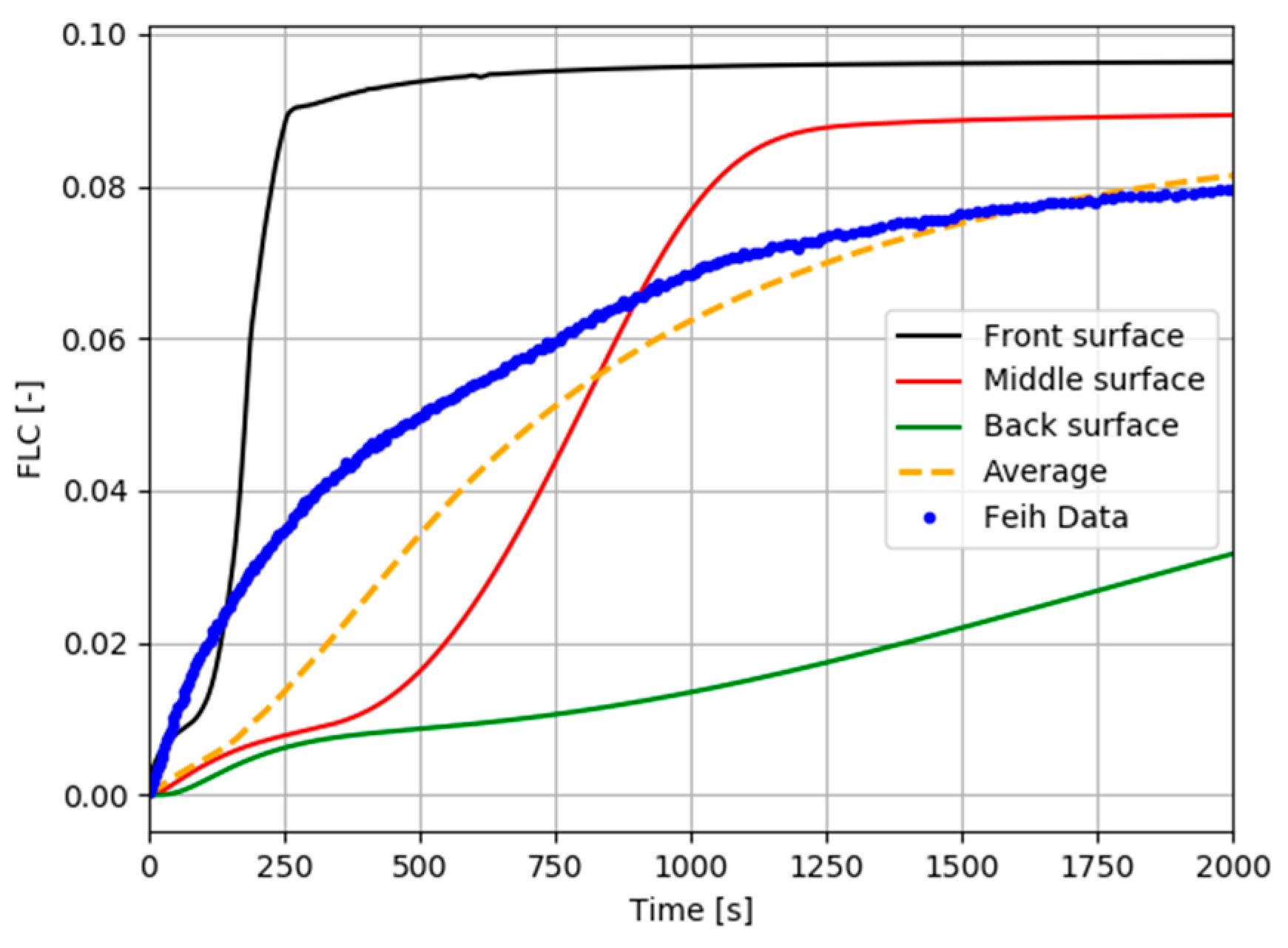
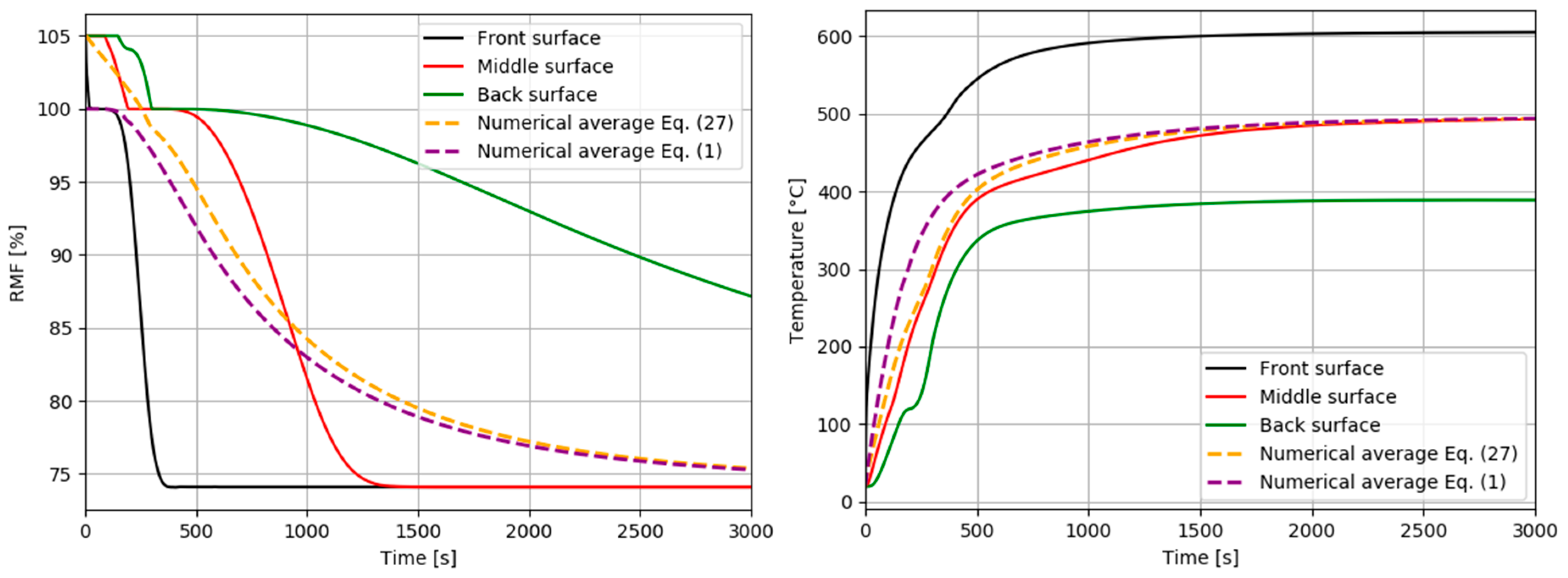
3.1. Thermal Degradation Prediction

The thermal degradation of three different composite materials was simulated. Temperature profiles and mass loss evolution were calculated using the thermal model exposed in the previous Section 2.1. These results are confronted with experimental data from other Authors [15,24,25] to probe and check the validity of our advanced thermal model. Other quantities of interest, such as internal pressure, gas storage or permeability profiles are available with the present model, but they are hardly comparable with experimental data, due to difficulty met for characterizing these parameters in practice.

The first material consists of a 9 mm-thick laminate made of plain woven E-glass fabric (800 g/m²) and vinyl ester resin (Derakane 411-350; Ashland Composite Polymers, Covington, KY, USA), which does not contain flame retardant fillers or additives. The fiber stacking sequence of the laminate is [0/90] and the fraction volume of fibers is 55%. It was used by Feih et al. [24] to validate their thermo-mechanical model, so similar properties were considered. Other properties related to thermal expansion, porosity, internal pressure, gas storage, and permeability were estimated using other bibliographic references. Thus, material data to run our thermal model are summed up in

Table 1. Material Properties for E-glass/vinyl ester composite laminate.

Property	Value	Source
Volume fraction of fibers (-)	0.55	[24]
Kinetics rate constant (1/s)	2 × 1013	[24]
Activation energy (J/mol)	2.12 × 105	[24]
Reaction order (-)	1	[24]
Remaining matrix mass fraction (-)	0.03	[24]
Heat of decomposition of the matrix (J/kg)	378,800	[24]
Density of glass fiber (kg/m3)	2560	[24]
Density of vinyl ester (kg/m3)	1140	[24]
Thermal conductivity of glass fiber (W/(m·K))	1.09	[24]
Thermal conductivity of vinyl ester (W/(m·K))	0.19	[26]
Specific heat of glass fiber (J/(kg·K))	760	[24]
Specific heat of vinyl ester (J/(kg·K))	1509	[17]
Initial specific heat of glass/vinyl ester (J/(kg·K))	960	[24]
Final specific heat of glass/vinyl ester (J/(kg·K))	1360	[24]
Specific heat of gas (vinyl ester) (J/(kg·K))	2386.5	[24]
Coefficient of convection (frontal surface) (W/(m2·K))	15	[25]
Coefficient of convection (back surface) (W/(m2·K))	0	[25]
Radiation source emissivity (-)	0.8	[25]
Emissivity of the front surface (-)	0.8	[25]
Emissivity of the back surface (-)	0.4	[25]
Room temperature (°C)	20	[24]
Thickness of the sample (m)	9 × 10−3	[24]
Virgin coefficient of linear thermal expansion (1/K)	2.52 × 10−5	[27]
Char coefficient of linear thermal expansion (1/K)	6.3 × 10−5	[27]
Dimensionless expansion factor (-)	−7.778 × 10−2	[15]
Virgin material permeability (m2)	8.29 × 10−17	[28]
Char material permeability (m2)	1.56 × 10−10	[28]
Virgin coefficient of permeability (1/K)	0	[15]
Char coefficient of permeability (1/K)	0	[15]
Dimensionless permeability factor (-)	−225	[15]
Molecular weight of gases (kg/mol)	18.35 × 10−3	[15]
Room pressure (normal pressure) (Pa)	101,325	–
Pressure on the back surface (Pa)	101,325	–
Gas viscosity (Pa·s)	1.5 × 10−5	[15]

.

For a heat flux of 50 kW/m², the thermal model provides the numerical thermal response of laminate exposed to fire. Figure 3 shows the mass loss and temperature profiles as a function of time, through laminate thickness, for three representative surfaces of the sample (front: x = 0 mm; middle: x = 4.5 mm; and back: x = 9 mm surface). We included in the graphics a numerical average curve (100 integration points through thickness) and experimental results measured by Feih et al. [24].

The mass loss shown in Figure 3 represents the amount of matrix that is thermally decomposed when the laminate is exposed to a constant heat flux. As the matrix decomposes, it releases volatile substances that reduce the mass of the laminate. As the decomposition rate of the matrix increases, it releases volatile gases at a faster rate (heat release rate), which is measured by an increase in the rate of mass loss.

The kinetics of mass loss is relatively fast for our prediction for a heat flux of 50 kW/m², but it is in very strong agreement with the measured values from the literature [24]. These material kinetics cause sufficiently high temperatures, which induce complete decomposition of the polymer matrix. For a heat flux of 50 kW/m², we observe very fast kinetics at the beginning of exposure to the heat flux, with maximum temperatures reached within 1000 s approximately. For a long enough exposure time, leading to a stationary temperature, the laminate is heated to a maximum temperature of about 600 °C on the upper front surface and at a minimum temperature of about 425 °C on the lower back surface, as shown in Figure 3. This is a consequence of the thermal conductivity decrease during the material degradation and also of the porosity creation and volume fraction increase, which are two parameters accounted for in the numerical thermal model.

Comparing the remaining mass fraction and temperature profiles shown in Figure 3, it could be seen that the loss of mass begins at the frontal surface starting from a temperature of about 350 °C, which means that the vinyl ester matrix does not decompose below this temperature. A decomposition gradient of the matrix is observed as a function of the exposure time and the through-thickness coordinate, so that the decomposition is slower when it moves away from the frontal surface directly in contact with the radiative hot source.

The thermal model enables the evaluation of other variables that are not available with typical thermal models presented in the literature [13,14,24,25], such as thermal expansion, density (modified by the volume change in the through-thickness direction), gas mass storage, permeability, porosity volume fraction, and internal pressure change. Figure 4 and Figure 5 present the evolution of thermal expansion through the fraction length change (FLC) and the internal pressure rise, respectively, for the E-glass/vinyl ester material submitted to a heat flux of 50 kW/m².

The FLC in Figure 4 represents the thermal deformation in the through-thickness direction. Strong agreement is obtained between the numerical average curve and the experimental curve published by Feih et al. [24]. The laminate expands continuously during exposure to a constant heat flux. However, the expansion rate slows down with time. Expansion profiles depend on temperature and degradation in Equation 6, so that the hot surface expands more rapidly at first and reaches the maximal expansion much more rapidly than the middle and back surface, respectively, where the material decomposition reaction advances more slowly. The internal pressure shown in Figure 5 is also dependent on the process of material degradation. The maximum pressure is predicted just after the onset of material decomposition, when the porosity is still low but the permeability is greater than the final permeability of the carbonized material. After reaching an absolute maximum, the internal pressure decreases within the material until it returns to ambient pressure. This is because the amount of volatiles decreases in the bulk of material due to the flow of gas to the outer surface where it is eventually evacuated in the ambient environment.

In order to ensure the validation and robustness of the present thermal model, another laminate was modeled. We simulated the thermal behavior of a different laminate made of E-glass fiber mat (800 g/m²) and an unsaturated polyester resin, with a hardener of methyl ethyl ketone (MEK) peroxide, which must be mixed with resin at a resin to MEK weight ratio of 100:1. The thickness of the composite laminate is 3.5 mm, as is the one used by Zhuge et al. [25], in order to validate their thermal model.

Table 2. Material properties for E-glass/polyester composite laminate.

Property	Value	Source
Fraction volume of fibers (-)	0.3	[25]
Kinetics rate constant (1/s)	1000	[25]
Activation energy (J/mol)	5 × 104	[25]
Reaction order (-)	1	[25]
Remaining matrix mass fraction (-)	0.01	[25]
Heat of decomposition of the matrix (J/kg)	−234,460	[25]
Density of glass fiber (kg/m3)	2694.7	[25]
Density of polyester (kg/m3)	1102.4	[25]
Thermal conductivity of glass fiber (W/(m·K))	1.04	[25]
Thermal conductivity of polyester (W/(m·K))	0.20	[25]
Specific heat of glass fiber (J/(kg·K))	760	[25]
Specific heat of polyester (J/(kg·K))	1600	[25]
Specific heat of gas (polyester) (J/(kg·K))	2386.5	[24]
Coefficient of convection (frontal surface) (W/(m2·K))	10	[25]
Coefficient of convection (back surface) (W/(m2·K))	0	[25]
Radiation source emissivity (-)	0.97	[25]
Emissivity of the front surface (-)	0.8	[25]
Emissivity of the back surface (-)	0.4	[25]
Room temperature (°C)	20	[25]
Thickness of the sample (m)	3.5 × 10−3	[25]
Virgin coefficient of linear thermal expansion (1/K)	9 × 10−6	[29]
Char coefficient of linear thermal expansion (1/K)	1.1 × 10−5	[29]
Dimensionless expansion factor (-)	−1 × 10−1	[15]
Virgin material permeability (m2)	3.19 × 10−16	[28]
Char material permeability (m2)	1 × 10−10	[28]
Virgin coefficient of permeability (1/K)	0	[15]
Char coefficient of permeability (1/K)	0	[15]
Dimensionless permeability factor (-)	−225	[15]
Molecular weight of gases (kg/mol)	18.35 × 10−3	[15]
Room pressure (normal pressure) (Pa)	101,325	–
Pressure on the back surface (Pa)	101,325	–
Gas viscosity (Pa·s)	1.5 × 10−5	[15]

summarizes the material properties.

Numerical prediction of the thermal response was also obtained for a heat flux of 50 kW/m². Figure 6 presents the mass loss–time and temperature–time profiles for three representative surfaces of the sample (front: x = 0 mm; middle: x = 1.75 mm; and back: x = 3.5 mm). Experimental results measured by Zhuge et al. [25] are also superposed in these figures, showing the very strong agreement with our numerical results. The remaining mass fraction (RMF) in Figure 6 shows that polyester resin is completely decomposed by a heat flux of 50 kW/m² in a faster way than vinyl ester resin (Figure 3), because of different decomposition kinetic parameters and the thinner thickness of the sample compared to Figure 3, which is devoted to the 9 mm-thick E-glass/vinyl ester composite. Consequently, we observe in Figure 6 that the maximum temperature of each surface is reached faster in comparison with the E-glass/vinyl ester sample. Observed discrepancies between the average numerical temperature and the measured data might be due to the temperature sensor used in experimental tests, which measures a disturbed temperature after resin degradation is complete.

Very satisfactory agreements are obtained between numerical results and experimental data [24,25] enabling the validation of the present thermal degradation model for composite materials based on polymer matrixes. Previous results only consider matrix degradation, although the thermal model is able to be adapted for different temperature conditions in order to account for fiber decomposition too, appropriately modifying Equation (4) to simulate different phases of decomposition. Following this approach, we also predicted the thermal behavior of a 2.9 cm-thick laminate of glass fiber and a phenol-formaldehyde (phenolic) matrix exposed to a heat flux of 279.7 kW/m², similar to the analyzed material presented by Henderson et al. [15]. Thermal properties, transport properties, and boundary conditions are summarized in [15]. The authors measured temperature variations as a function of time in order to obtain the thermal response of the material in a suitable range of temperature up to around 1000 °C. Figure 7 shows the temperature–time profiles for four representative surfaces of the sample (x = 0.1 cm, x = 0.5 cm, x = 1 cm and back surface at x = 2.9 cm) and the average numerical curve of temperature, which is the normalized sum of all degradation states for each element in the through-thickness of the material. It also shows experimental results measured by Henderson et al. [15] at the same points. Again, the agreement between the measured and calculated temperatures is very strong for the heat flux of 279.7 kW/m².

All these results let us trust in our advanced thermal model to predict thermal behavior of polymer composite laminates exposed to a constant heat flux. Other conditions (different heat flux, fiber/matrix rate or laminate thickness) can be evaluated, predicted, and compared with this model.

3.2. Mechanical Properties Prediction

The temperature and mass loss profile predictions obtained in the previous section are used as input to calculate the post-combustion mechanical properties of composite materials. The combustion advancing front can be calculated for different rates of decomposition, supposing that the material reaches progressively a certain value of $\alpha \left(x,t\right)$ at each surface through the thickness direction. Then, we can calculate the normalized flexion modulus using Equation (20). Figure 8 shows the combustion advancing front for three different degradation rates: $\alpha \left(x,t\right)=0.5$ (intermediate decomposition), $\alpha \left(x,t\right)=0.1$ (almost total decomposition), and $\alpha \left(x,t\right)=0.9$ (low decomposition). Figure 9 shows a normalized flexural modulus. Both figures show a 3.5 mm-thick E-glass/polyester composite laminate, similar to the one presented in the previous section for a heat flux of 50 kW/m². Figure 9 also presents a comparison between experimental measured data obtained by Zhuge et al. [25] and our numerical results calculated with Equation (20), supposing three different degradation rates $\alpha \left(x,t\right)$ as a definition of combustion advancing front. It is observed in Figure 9 that the fall of the flexural modulus depends directly on the time of exposure to fire. In fact, the increase in the combustion time is related to the position of the advancing front of the combustion, as shown in Figure 8. Over time, the thickness of the carbonized layer increases, as well as its contribution to the overall properties of the composite laminate. One can observe that the experimental data of the normalized flexural modulus are located between a low and an intermediate decomposition of the matrix material (black and red curves respectively in Figure 9). One could appreciate that there are small differences between the numerical results and the experimental data at first instance. This is a consequence of the assumption of the definition of combustion advancing front for an intermediate state of decomposition, because theb normalized flexural modulus starts to reduce since material starts to decompose at the front region, even before we consider a change of the material behavior or the possible occurrence of damage [30]. It might be possible to obtain more accurate results with a more complex definition of combustion advancing front, such as a combination of all states of material degradation. However, the agreement of the curve considering a degradation rate $\alpha \left(x,t\right)=0.5$ with experimental data is good enough to validate the present approach for the prediction of post-combustion mechanical properties in polymer composite materials.

4. Discussion: Hygro-Thermal Durability in Fire Conditions

4.1. Hygro-Thermal Model Development

Water content in composite materials can considerably affect thermal behavior. Thus, the thermal model presented in Section 2 was improved in order to consider the water mass fraction that can be contained inside the material. It is important to consider this moisture absorption in composite materials as it can dramatically affect the durability and global properties (physical and mechanical) [31,32,33,34]. Moreover, depending on the nature of its polymer matrix, composite materials experiencing aging in humid environments could contain a possibly high moisture content prior to fire exposure. To our knowledge, combined hygro-thermal durability of composite materials submitted to fire conditions was never studied in the literature. Of course, one could find numerous hygro-thermal durability studies but for quite moderately high temperatures (until 200–250 °C) [35,36,37]. Due to the complexity of the problem, we made some additional assumptions to properly model the hygro-thermal response of polymer composite materials exposed to a constant heat flux, related to desorption mechanism. The initial water content is taken into account as an additional mass contribution to the control volume of the analyzed solid material. The problem is then treated as a law of mixtures with all the constituents of the materials, making it possible to define an equivalent homogeneous elementary volume. Water does not have a privileged position in the volume. We consider a first step of free water desorption. Free water does not form bonds with the molecular network of the matrix and will be assumed firstly to be stored in material porosities. Then, in a second step, bounded water is considered, which will be evacuated at slightly higher temperatures because of the weak bonds formed between these water molecules and the molecular network of the matrix.

Water desorption was modeled using Equation (22), which represents an additional equation to include in the PDE system to be solved. It is based on a dehydration equation proposed by Sand et al. [38], but this is modified and expressed as a partial differential equation for the water mass loss as a function of time, though-thickness coordinate, total mass of the composite, and instantaneous temperature:

$$\frac{\partial m_{H_{2}O}\left(x,t\right)}{\partial t}=-\frac{\partial }{\partial t}\left(\frac{m_{composite}\left(x,t\right) c_p\left(x,t\right)\left[T\left(x,t\right)-T_{sat}\right]}{\Delta h_{fg}\left(x,t\right)}\right).$$

(22)

In Equation (22), $m_{H_{2}O}\left(x,t\right)$ is the instantaneous water mass contained inside the material. $T_{sat}$ is the fiber’s saturation temperature, which is equal to the water evaporation temperature (T_sat = 373.15 K) in the first step of the desorption of free water (boiling water which has not formed any bonds with the polymer network). This temperature is considered to be slightly higher in the second step of bounded water and is calculated as the temperature at which the instantaneous mass fraction of water reaches the value $X_{fsp}$, which represents the water mass fraction at the fiber saturation point. $\Delta h_{fg}\left(x,t\right)$ is the latent heat of water, depending on temperature $T\left(x,t\right)$ and the water mass fraction $\left(X_{H_{2}O}\left(x,t\right)=\frac{m_{H_{2}O}\left(x,t\right)}{m_{composite}\left(x,t\right)}\right)$ for the step of desorption of bound water. It takes different expressions for free liquid and bound water [36] as proposed in Equation (23–26):

$$\Delta h_l\left(x,t\right)\left[J/kg\right]=1000\left[3179-2.5 T\left(x,t\right)\right],$$

(23)

$$\Delta h_{desorp}\left(x,t\right)\left[J/kg\right]=1000\left[1176.2e^{-15X_{H_{2}O}\left(x,t\right)}\right],$$

(24)

$$\Delta h_{fg}\left(x,t\right)=\Delta h_l\left(x,t\right)\mathrm{for} X_{H_{2}O}\left(x,t\right)\ge X_{fsp},$$

(25)

$$\Delta h_{fg}\left(x,t\right)=\Delta h_l\left(x,t\right)+\Delta h_{desorp}\left(x,t\right)\mathrm{for} X_{H_{2}O}\left(x,t\right)<X_{fsp}.$$

(26)

With Equation (23–26), one can explain the processes of composite material dehydration. For the first step of free water desorption, only evaporation heat $\Delta h_l\left(x,t\right)$ of free liquid water is required up to $X_{fsp}$. Then, for the second step, which corresponds to bound water desorption, an additional heat of desorption $\Delta h_{desorp}\left(x,t\right)$ must be introduced to account for the energy necessary to break the weak bonds existing between water molecules and the matrix network.

Following this approach, it is possible to express the water mass loss in a similar way as resin mass loss. That is schematized in Figure 10: Each volume element consists now of an amount of fibers (black cylinder), an amount of matrix (orange), an amount of air porosity (light blue), and an amount of water (dark blue). The numerical solution of the problem allows us to evaluate the influence of the water content on the hygro-thermal response of composite materials.

The heat equation (Equation (1)) must be modified in order to explicitly consider the water content:

$$\begin{array}{c}[m_{composite}(x,t)(c_p(x,t)+c_{pv{H}_{2}O}(x,t))+m_g(x,t)c_{pg}(x,t)]\frac{\partial T(x,t)}{\partial t}=\frac{\partial }{\partial x}\{[k_g(x,t)\varphi (x,t)+\\ k_x(x,t)(1-\varphi (x,t))]\frac{\partial T(x,t)}{\partial x}\}\Delta x(x,t)\Delta A-{\dot{m}}_{gtotal}(x,t)c_{pg}(x,t)\frac{\partial T(x,t)}{\partial x}\Delta x(x,t)-\\ \frac{\partial m_{composite}(x,t)}{\partial t}[Q_p+h_s(x,t)-h_g(x,t)-h_{v{H}_{2}O}(x,t)],\end{array}$$

(27)

with

$$m_{composite}\left(x,t\right)=m_m\left(x,t\right)+m_{fiber}+m_{H_{2}O}\left(x,t\right),$$

(28)

and

$${\dot{m}}_{gtotal}\left(x,t\right)={\dot{m}}_g\left(x,t\right)+{\dot{m}}_{v{H}_{2}O}\left(x,t\right),$$

(29)

and

$$\frac{\partial m_{composite}\left(x,t\right)}{\partial t}=m_{composite}\left(x,t\right) A {\left[\alpha \left(x,t\right)\right]}^n{e}^{-\frac{E_a}{R T\left(x,t\right)}}\mathrm{for} m_{H_{2}O}\left(x,t\right)=0.$$

(30)

In Equation (27), the influence of water is explicitly considered in the total mass of the composite and in the production rate of volatiles, which consists in water vapor because of material desorption, and lastly, gases that flow due to the pyrolysis reaction and matrix decomposition. The specific heat of the composite material was modified by adding an additional contribution of the water mass contained in the material [39] due to the modeling of the loss of water mass as a simple mechanism of evaporation depending on the temperature:

$$c_{pv{H}_{2}O}\left(x,t\right)=\frac{f_c \Delta h_{fg}\left(x,t\right) X_{H_{2}O}\left(x,t\right)}{T\left(x,t\right)-T_{sat}}.$$

(31)

In Equation (31), $f_c$ is a correction factor that is introduced in order to account for additional energy due to the dehydration process. Finally, $c_{p{H}_{2}O}\left(x,t\right)$ allows us to calculate an additional contribution to enthalpy $h_{v{H}_{2}O}\left(x,t\right)$, which must be included in Equation (27) to ensure the energy conservation.

The mass conservation equation (Equation (8)) must be adapted in order to consider the water mass contribution. This enables us to distinguish the calculation of volatiles mass storage, pressure of evaporation, and matrix decomposition processes, in order to evaluate individually the contribution of each process, as shown in Equation (32–34):

$$-\frac{\partial m_{composite}\left(x,t\right)}{\partial t}=\frac{\partial m_g\left(x,t\right)}{\partial t}+\frac{\partial {\dot{m}}_g\left(x,t\right)}{\partial t}\Delta x\left(x,t\right)+\frac{\partial m_{v{H}_{2}O}\left(x,t\right)}{\partial t}+\frac{\partial {\dot{m}}_{v{H}_{2}O}\left(x,t\right)}{\partial t}\Delta x\left(x,t\right),$$

(32)

$$-\frac{\partial \left(m_m\left(x,t\right)+m_{fiber}\right)}{\partial t}=\frac{\partial m_g\left(x,t\right)}{\partial t}+\frac{\partial {\dot{m}}_g\left(x,t\right)}{\partial t}\Delta x\left(x,t\right),$$

(33)

$$-\frac{\partial m_{H_{2}O}\left(x,t\right)}{\partial t}=\frac{\partial m_{v{H}_{2}O}\left(x,t\right)}{\partial t}+\frac{\partial {\dot{m}}_{v{H}_{2}O}\left(x,t\right)}{\partial t}\Delta x\left(x,t\right),$$

(34)

with the subscripts g and $v{H}_{2}O$ referring to gases produced by matrix decomposition and water vapor, respectively. Thus, pressure is calculated following the procedure presented in Section 2.1 for the pyrolysis process and for the first step of desorption process up to $X_{fsp}$. For the second step of bound water desorption, the pressure is calculated following Equation (35), with $P_{v{H}_{2}O}^{sat}$ referring to the saturation pressure, when $X_{H_{2}O}\left(x,t\right)=X_{fsp}$:

$$P_{v{H}_{2}O}\left(x,t\right)=P_{v{H}_{2}O}^{sat} \left[1-{\left(1-\frac{ X_{H_{2}O}\left(x,t\right)}{X_{fsp}}\right)}^{6.453·{10}^{-3} T\left(x,t\right)}\right] \mathrm{for} X_{H_{2}O}\left(x,t\right)<X_{fsp}.$$

(35)

In order to obtain the hygro-thermal problem in a mathematically resoluble system of PDEs, it is necessary to include new initial and boundary conditions that involve the new variables related to water content. These new conditions are summarized in Equation (36) and Equation (37):

$$\begin{gathered} m_{H_{2}O}\left(x,0\right)=m_{H_{2}O0}, m_{v{H}_{2}O}\left(x,0\right)=m_{v{H}_{2}O0}, {\dot{m}}_{v{H}_{2}O}\left(x,0\right)=0, P_{v{H}_{2}O}\left(x,0\right)=P_{v{H}_{2}O0} \\ \mathrm{for} 0\le x\le L, \end{gathered}$$

(36)

$${\dot{m}}_{v{H}_{2}O}\left(L,t\right)=0, P\left(L,t\right)=P_s\mathrm{for} x=L \mathrm{and} \forall t>0.$$

(37)

This new formulation of the hygro-thermal problem lets us obtain the temporal and through-thickness evolution of all variables involved, such as thermal expansion, internal pressure, porosity, gas flux rate, gas mass storage, and permeability. In addition, the possibility to predict the evolution of all these parameters depending on the amount of water introduced into the material constitutes the highlight of our advanced model. Obviously, temperature and matrix mass loss profiles are influenced by water content. This information about the hygro-thermal behavior of laminated composite material is used to calculate the evolution of post-combustion mechanical properties through the numerical model presented in Section 2.2, which makes it possible to predict the durability of composite materials exposed to fire after having been aged in humid environmental conditions. It is also possible to consider a gradient of water content inside the composite material, which could simulate a wall in contact with two different environments. Numerical results are discussed in the next section.

4.2. Hygro-Thermo-Mechanical Durability

Numerical results were obtained using the hygro-thermal model for a heat flux of 50 kW/m² applied on a 9 mm-thick E-glass/vinyl ester and a 3.5 mm-thick E-glass/polyester composite laminate (similar to the one introduced in Section 3.2), of which the material properties are shown in Table 1 and Table 2, respectively.

Figure 11 presents the mass loss–time (remaining mass fraction) and temperature–time profiles at three representative surfaces of the E-glass/vinyl ester sample (front: x = 0 mm; middle: x = 4.5 mm; and back: x = 9 mm), with an initial water mass fraction content of 5% related to the solid mass of the laminate. We observe a first step of mass loss due to the material desorption from about 100 °C (water vaporization temperature), followed by a second decrease of mass due to the decomposition of the matrix by pyrolysis. The numerical average curve (orange discontinued line) is confronted against the average curve (purple discontinued line) from the previous thermal model (without water content consideration) presented in Section 3.2 in order to analyze the influence of water content. We notice in Figure 11 that matrix degradation is slower in the wet sample because of coupling between water desorption and pyrolysis reaction, of which the kinetics are different. Consequently, the evolution of temperature is also slower, particularly at the beginning of fire exposure, due to consummation of a part of the heat flux energy in order to produce the water evaporation.

An analogous study was carried out for the E-glass/polyester material exposed to a heat flux of 50 kW/m², with an initial water mass fraction content of 5% related to the solid mass of the laminate. Mass loss–time (remaining mass fraction) and temperature–time profiles are shown in Figure 12 for three representative surfaces of the sample (front: x = 0 mm; middle: x = 1.75 mm; and back: x = 3.5 mm). We observe, compared to the other material, the influence of considering water content in a hygro-thermal model, thanks to the comparison against a thermal model of numerical average results. This is due to thinner thickness and different kinetic parameters of the pyrolysis reaction compared to the E-glass/vinyl ester laminate. The mass loss and the increase of temperature of wet laminate (orange discontinued line) slow down compared to the dry specimen (purple discontinued line) due to the effect of evaporation process, which involves a significant consummation of initial heat flux energy.

Consistent results using a hygro-thermal model were obtained, which justifies assumptions made in Section 4.1 to formulate it. However, an experimental validation is envisaged in forthcoming works to validate numerical predictions.

The presented hygro-thermal model is able to predict the hygro-thermal behavior of polymer composite materials through a relatively simple approach, taking into account the evolution of water content through the material thickness as an additional variable of the thermal problem. Consequently, we can predict post-combustion mechanical properties for wet composite materials in a similar way to the methodology presented in Section 3.1 for dry composite materials. Indeed, water content modifies the thermal answer during the combustion and, therefore, post-fire mechanical properties are directly influenced by water content. Figure 13 shows the combustion advancing front defined for a degradation rate of 50%, corresponding to $\alpha \left(x,t\right)=0.5$ (intermediate decomposition) and Figure 14 shows a normalized flexural modulus, with both figures representing a 3.5 mm-thick E-glass/polyester composite laminate and a heat flux of 50 kW/m². Numerical results are superposed for a dry material and a wet material having an initial water mass fraction content of 5%, in order to compare them.

One could observe that the combustion advancing front and the normalized flexural modulus in the case of the wet material are both offset in time with respect to the predictions obtained for the dry material. This effect is due to the evaporation process of water, as it can obviously be predicted from the thermal degradation and temperature results shown in Figure 12. It is observed that a significant initial water content (green curves) slows down the rise of temperature, due to the fact that the water captures part of the incident heat flux, which is consumed to heat the water and vaporize it. This limits the heating of the composite, firstly as observed in Figure 12 and, as a consequence, the times of combustion and failure in flexion increase with respect to dry samples (black curves). Thus, the hygro-thermal model presented here enables the accurate prediction of post-combustion mechanical properties for composite laminates with an initially wet polymer matrix.

5. Conclusions

The present results show that the fire thermal response and decomposition of polymer composite laminates depend on several parameters that are strongly coupled to each other. A numerical 1D thermal model was developed considering the main phenomena concerning the exposure to fire of composite materials. The thermal decomposition of matrix and fibers and temperature fields can be evaluated as a function of time and of through-thickness coordinate. Other variables such as thermal expansion, internal pressure, porosity, gas flux rate, gas mass storage, and permeability are available with the present advanced thermal model. Taking these parameters into account is important because they directly and strongly affect, as shown in the numerical cases provided in this work, the time-dependent through-thickness temperature field. A more complex hygro-thermal model was developed in order to consider the effects related to the presence of an initial water content field within the polymer matrix. This is of outmost importance for understanding the durability of composite materials and the evolution of their properties, especially in a high temperature environment. Water was observed to act as a thermal barrier, which leads to a slower degradation and evolution of temperature, as a consequence of energy consumption during the water evaporation process. This last model enables to estimate the hygro-thermal durability in order to predict the combustion advancing front in extreme conditions of temperature and moisture, leading to the estimation of the material post-combustion mechanical properties. Numerical results were compared to literature for dry laminates showing an excellent agreement between both. However, such a comparison between our numerical simulation and measured data for a moisturized material could not be made due to a lack of measured data in the literature, this field of study being completely new. Mechanical properties are directly dependent of the thermal response of the material. It is thus envisaged to include explicitly mechanical aspects such as matrix-fiber debonding, matrix cracking, or ply delamination into the present numerical thermal model. In addition, thermal properties were defined as homogeneous laws, but they could be defined more precisely at the ply scale or even at the individual constituent scale as a function of temperature and of the degradation rate. Despite required improvement, the advanced model proposed in this paper enables one to predict the fire response of composite laminates at the macroscopic scale (post-combustion properties), from the local through-thickness estimates of temperature fields and degradation. The model presented here concerns a first approach to predict materials hygro-thermo-chemico-mechanical durability in severe conditions of temperature, providing a better understanding of the effects related to many parameters, such as thermal expansion, density (modified by the volume change in the through-thickness direction), gas mass storage, permeability, porosity, internal pressure, moisture content (free and bounded water), combustion advancing front, mechanical properties, etc. This is the first step to evaluate the behavior of composite materials from a more realistic point of view, which becomes important to assess the material behavior at the microscopic scale. The second step is to use the predictions obtained by our model to improve the properties and better design laminated composite materials. Indeed, our advanced numerical model makes it possible to obtain reliable results regarding the evolution of the thermo-mechanical properties as a function of the porosity rate (air), the quantity of water diffused or of other type of impurity rate (which can be treated as a different porosity having the properties of such or such resin). Our model then enables performing test-and-error tests, allowing an industrialist to save time and money by only changing a few material solutions through reliability tests. The present work was focused on the hygro-thermo-chemico-mechanical durability of fiber-reinforced polymer composites exposed to fire. We also develop a new hygro-thermo-chemico-mechanical model, based on the same approach with additional specificities, in the case of a balsa core sandwich composite material, taking into account water desorption and infused resin degradation into the balsa core.

References

1. Legrand, V.; Merdrignac-Conanec, O.; Paulus, W.; Hansen, T. Study of the thermal nitridation of nanocrystalline Ti(OH)4 by X-ray and in situ neutron powder diffraction. J. Phys. Chem. A 2012, 116, 9561–9567. [Google Scholar] [CrossRef]
2. Legrand, V.; Pillet, S.; Weber, H.P.; Souhassou, M.; Létard, J.-F.; Guionneau, P.; Lecomte, C. On the precision and accuracy of structural analysis of light induced metastable states. J. Appl. Crystallogr. 2007, 40, 1076–1088. [Google Scholar] [CrossRef]
3. Legrand, V.; Pillet, S.; Carbonera, C.; Souhassou, M.; Létard, J.-F.; Guionneau, P.; Lecomte, C. Optical, magnetic and structural properties of the spin crossover complex [Fe(btr)2(NCS)2].H2O in the light-induced and thermally quenched metastable states. Eur. J. Inorg. Chem. 2007, 5693–5706. [Google Scholar] [CrossRef]
4. Legrand, V.; Carbonera, C.; Pillet, S.; Souhassou, M.; Létard, J.-F.; Guionneau, P.; Lecomte, C. Photocrystallography: From the structure towards the electron density of metastable states. J. Phys. Conf. Ser. 2005, 21, 73–80. [Google Scholar] [CrossRef]
5. Gloaguen, D.; Oum, G.; Legrand, V.; Fajoui, J.; Moya, M.J.; Pirling, T.; Kockelmann, W. Intergranular strain evolution in titanium during tensile loading: Neutron diffraction and polycristalline model. Metall. Mater. Trans. A 2015, 46, 5038–5046. [Google Scholar] [CrossRef]
6. Hounkpati, V.; Fréour, S.; Gloaguen, D.; Legrand, V.; Kelleher, J.; Kockelmann, W.; Kabra, S. In situ neutron measurements and modelling of the intergranular strains in the near- titanium alloy Ti-β21S. Acta Mater. 2016, 109, 341–352. [Google Scholar] [CrossRef]
7. Legrand, V.; Kockelmann, W.; Frost, C.D.; Hauser, R.; Kaczorowski, D. Neutron diffraction study of the non-Fermi liquid compound CeNiGa2: Magnetic behaviour as a function of pressure and temperature. J. Phys. Condens. Matter 2013, 25, 206001. [Google Scholar] [CrossRef]
8. Legrand, V.; Le Gac, F.; Guionneau, P.; Létard, J.-F. Neutron powder diffraction studies of two spin transition Fe(II)-complexes under pressure. J. Appl. Crystallogr. 2008, 41, 637–640. [Google Scholar] [CrossRef]
9. Legrand, V.; Pechev, S.; Létard, J.-F.; Guionneau, P. Synergy between polymorphism, pressure, spin-crossover and temperature in [Fe(PM-BiA)2(NCS)2]: A neutron powder diffraction investigation. Phys. Chem. Chem. Phys. 2013, 15, 13872–13880. [Google Scholar] [CrossRef]
10. Legrand, V.; Pillet, S.; Souhassou, M.; Lugan, N.; Lecomte, C. Extension of the experimental electron density analysis to metastable states: A case example of the spin crossover complex Fe(btr)2(NCS)2.H2O. J. Am. Chem. Soc. 2006, 128, 13921–13931. [Google Scholar] [CrossRef]
11. Rizk, G.; Legrand, V.; Khalil, K.; Casari, P.; Jacquemin, F. Durability of sandwich composites under extreme conditions: Towards the prediction of fire resistance properties based on thermo-mechanical measurements. Compos. Struct. 2018, 186, 233–245. [Google Scholar] [CrossRef]
12. Mouritz, A.P.; Gibson, A.G. Fire Properties of Polymer Composite Materials, Solid Mechanics and Its Applications; Springer: Berlin/Heidelberg, Germany, 2006. [Google Scholar]
13. Henderson, J.B.; Wiebelt, J.A.; Tant, M.R. A model for the thermal response of polymer composite materials with experimental verification. J. Compos. Mater. 1985, 19, 579–595. [Google Scholar] [CrossRef]
14. Gibson, A.G.; Wu, Y.-S.; Chandler, H.W.; Wilcox, J.A.D.; Bettess, P. A model for the thermal performance of thick composite laminates in hydrocarbon fires. Rev. L’Inst. Fr. Pét. 1995, 50, 69–74. [Google Scholar] [CrossRef]
15. Henderson, J.B.; Wiecek, T.E. A Mathematical Model to Predict the Thermal Response of Decomposing, Expanding Polymer Composites. J. Compos. Mater. 1986, 21, 373–393. [Google Scholar] [CrossRef]
16. Buch, J.D. Thermal Expansion Behavior of a Thermally Degrading Organic Matrix Composite. In Thermomechanical Behavior of High-Temperature Composites; ASME Publication AD-04; ASME: New York, NY, USA, 1982. [Google Scholar]
17. Lattimer, B.Y.; Ouellette, J.; Trelles, J. Thermal Response of Composite Materials to Elevated Temperatures. Fire Technol. 2011, 47, 823–850. [Google Scholar] [CrossRef]
18. Ramroth, W.T. Thermo-Mechanical Structural Modelling of FRP Composite Sandwich Panels Exposed to Fire. Ph.D. Thesis, UC San Diego, San Diego, CA, USA, 2006. [Google Scholar]
19. The Numerical Method of Lines. Available online: https://reference.wolfram.com/language/tutorial/NDSolveMethodOfLines.html (accessed on 1 September 2017).
20. Mouritz, A.P.; Mathys, Z. Post-fire mechanical properties of marine polymer composites. Compos. Struct. 1999, 47, 643–653. [Google Scholar] [CrossRef]
21. Mouritz, A.P.; Mathys, Z. Post-fire mechanical properties of glass-reinforced polyester composites. Compos. Sci. Technol. 2001, 61, 475–490. [Google Scholar] [CrossRef]
22. Mouritz, A.P.; Feih, S.; Kandare, E.; Mathys, Z.; Gibson, A.G.; Des Jardin, P.E.; Case, S.W.; Lattimer, B.Y. Review of fire structural modelling of polymer composites. Compos. Part A 2009, 40, 1800–1814. [Google Scholar] [CrossRef]
23. Theulen, J.C.M.; Peijs, A.A.J.M. Optimization of the bending stiffness and strength of composite sandwich panels. Compos. Struct. 1991, 17, 87–92. [Google Scholar] [CrossRef] [Green Version]
24. Feih, S.; Mathys, Z.; Gibson, A.G.; Mouritz, A.P. Modelling the compression strength of polymer laminates in fire. Compos. Part A 2007, 38, 2354–2365. [Google Scholar] [CrossRef]
25. Zhuge, J.; Gou, J.; Chen, R.-H.; Kapat, J. Finite element modeling of post-fire flexural modulus of fiber reinforced polymer composites under constant heat flux. Compos. Part A 2012, 43, 665–674. [Google Scholar] [CrossRef]
26. Overall Heat Transfer Coefficient. Available online: https://www.engineeringtoolbox.com/overall-heat-transfer-coefficient-d_434.html (accessed on 1 September 2017).
27. Vinyl Ester Systems. Available online: https://www.epoxy.com/vester.htm (accessed on 1 September 2017).
28. Goodrich, T.W.; Lattimer, B.Y.; Case, S.W.; Ellis, M.W. Thermophysical Properties and Microstructural Changes of Composite Materials at Elevated Temperature. Ph.D. Thesis, Faculty of the Virginia Polytechnic Institute and State University, Blacksburg, VA, USA, 2009. [Google Scholar]
29. Polyester Resins. Available online: http://www.exelcomposites.com/fi-fi/english/composites/rawmaterials/resins.aspx (accessed on 1 September 2017).
30. Mouritz, A.P.; Feih, S.; Kandare, E.; Mathys, Z.; Gibson, A.G.; Des Jardin, P.; Case, S.; Lattimer, B. Damage and failure modelling of fibre-polymer composite in fire. Int. Conf. Compos. Mater. 2009. [Google Scholar]
31. Youssef, G.; Fréour, S.; Jacquemin, F. Stress-dependent Moisture Diffusion in Composite Materials. J. Compos. Mater. 2009, 43, 1621–1637. [Google Scholar] [CrossRef]
32. Ramezani Dana, H.; Jacquemin, F.; Fréour, S.; Perronnet, A.; Casari, P.; Lupi, C. Numerical and experimental investigation of hygro mechanical states of glass fiber reinforced polyester composites experienced by FBG sensors. Compos. Struct. 2014, 116, 38–47. [Google Scholar] [CrossRef] [Green Version]
33. Ibrahim, G.; Casari, P.; Jacquemin, F.; Fréour, S.; Clement, A.; Célino, A.; Khalil, K. Moisture diffusion in composites tubes: Characterization and identification of microstructure-properties relationship. J. Compos. Mater. 2018, 52, 1073–1088. [Google Scholar] [CrossRef]
34. Shi, X.; Xiao, H.; Liao, X.; Armstrong, M.; Chen, X.; Lackner, K.L. Humidity effect on ion behaviors of moisture-driven CO2 sorbents. J. Chem. Phys. 2018, 149, 164708. [Google Scholar] [CrossRef] [PubMed]
35. Peters, B.; Bruch, C. A flexible and stable numerical method for simulating the thermal decomposition of wood particles. Chemosphere 2001, 42, 481–490. [Google Scholar] [CrossRef]
36. Bryden, K.M.; Ragland, K.W.; Rutland, C.J. Modeling thermally thick pyrolysis of wood. Biomass Bioenergy 2002, 22, 41–53. [Google Scholar] [CrossRef]
37. Shi, L.; Michael, Y.L.C. A review of fire processes modeling of combustible materials under external heat flux. Fuel 2013, 106, 30–50. [Google Scholar] [CrossRef]
38. Sand, U.; Sandberg, J.; Larfeldt, J.; Bel Fdhila, R. Numerical prediction of the transport and pyrolysis in the interior and surrounding of dry and wet wood log. Appl. Energy 2008, 85, 1208–1224. [Google Scholar] [CrossRef]
39. Looyeh, M.R.E.; Bettess, P. A Finite element model for the fire-performance of GRP panels including variable thermal properties. Finite Elem. Anal. Des. 1998, 30, 313–324. [Google Scholar] [CrossRef]
Figure 1. Schematic of thermal expansion modeling of a laminated composite material.
Jcs 03 00055 g001
Figure 2. Scheme of the idealized two-layer model for studying the post-combustion mechanical properties of a laminated composite material (for clarity reason, only one part of the fiber is represented).
Jcs 03 00055 g002
Figure 3. Remaining mass fraction (RMF) profiles and temperature profiles. Comparison between our numerical simulation predictions (label surface) as a function of time to the experimental data of Feih et al. [24] (label surface data) for an E-glass/vinyl ester composite laminate exposed to a heat flux of 50 kW/m2.
Jcs 03 00055 g003
Figure 4. E-glass/vinyl ester material submitted to a heat flux of 50 kW/m2; thermal through-thickness expansion profiles (fraction length change, FLC).
Jcs 03 00055 g004
Figure 5. E-glass/vinyl ester material exposed to a heat flux of 50 kW/m2; internal pressure profiles.
Jcs 03 00055 g005
Figure 6. Remaining mass fraction (RMF) profiles and temperature profiles. Comparison between our numerical simulation prediction as a function of time and the experimental data of Zhuge et al. [25] for an E-glass/ polyester composite laminate at a heat flux of 50 kW/m2.
Jcs 03 00055 g006
Figure 7. Prediction of temperature profiles. Comparison between the numerical simulation prediction (continuous lines) as a function of time and the experimental data of Henderson et al. [15] (discontinuous points) for a glass-filled/phenolic composite laminate exposed to a heat flux of 279.7 kW/m2.
Jcs 03 00055 g007
Figure 8. Numerical simulation to predict the combustion advancing front for different degradation rates for an E-glass/polyester composite laminate and a heat flux of 50 kW/m2.
Jcs 03 00055 g008
Figure 9. Normalized flexural modulus as a function of combustion time for an E-glass/polyester composite laminate and a heat flux of 50 kW/m2. Comparison between numerical simulation prediction (discontinuous curves) and experimental data (▲) obtained by Zhuge et al. [25].
Jcs 03 00055 g009
Figure 10. Schematic of hygro-thermal expansion modeling of a laminated composite material. Each volume element is formed by fibers, matrix resin, porosity, and water (free and bonded).
Jcs 03 00055 g010
Figure 11. Remaining mass fraction (RMF) profiles and temperature profiles through the material thickness as a function of time. Comparison of numerical simulation prediction as a function of time between thermal and hygro-thermal models for a 9 mm-thick E-glass/vinyl ester composite laminate exposed at a heat flux of 50 kW/m2.
Jcs 03 00055 g011
Figure 12. Remaining mass fraction (RMF) profiles and temperature profiles through the material thickness as a function of time. Comparison of numerical simulation prediction as a function of time between thermal and hygro-thermal models for a 3.5 mm thickness E-Glass/polyester composite laminate exposed to a heat flux of 50 kW/m2.
Jcs 03 00055 g012
Figure 13. Kinetics of the combustion advancing front for a degradation rate of 50%. Comparison of numerical simulation prediction as a function of combustion time between pure thermal and hygro-thermal models for an E-glass/polyester composite laminate exposed to a heat flux of 50 kW/m2.
Jcs 03 00055 g013
Figure 14. Post-combustion time dependence of the normalized flexural modulus for a degradation rate of 50%. Comparison of numerical simulation prediction as a function of combustion time between pure thermal and hygro-thermal models for an E-glass/polyester composite laminate and a heat flux of 50 kW/m2. Experimental data (▲, dry material) obtained by Zhuge et al. [25] are also reported.
Jcs 03 00055 g014