Variable Stiffness Composites: Optimal Design Studies
by
 and
and
Filipe Eduardo Correia Marques
1, 
Ana Filipa Santos da Mota
1,2 and
Maria Amélia Ramos Loja
1,2,3,* 1
CIMOSM, ISEL, Centro de Investigação em Modelação e Optimização de Sistemas Multifuncionais, 1959-007 Lisboa, Portugal
2
Universidade de Évora, 7000-671 Évora, Portugal
3
IDMEC, IST—Instituto Superior Técnico, Universidade de Lisboa, 1049-001 Lisboa, Portugal
*
Author to whom correspondence should be addressed.
J. Compos. Sci. 2020, 4(2), 80; https://doi.org/10.3390/jcs4020080
Submission received: 24 May 2020
/
Revised: 19 June 2020
/
Accepted: 20 June 2020
/
Published: 24 June 2020
(This article belongs to the Special Issue Feature Papers in Journal of Composites Science in 2020)
Abstract
:This research work has two main objectives, being the first related to the characterization of variable stiffness composite plates’ behavior by carrying out a comprehensive set of analyses. The second objective aims at obtaining the optimal fiber paths, hence the characteristic angles associated to its definition, that yield maximum fundamental frequencies, maximum critical buckling loads, or minimum transverse deflections, both for a single ply and for a three-ply variable stiffness composite. To these purposes one considered the use of the first order shear deformation theory in connection to an adaptive single objective method. From the optimization studies performed it was possible to conclude that significant behavior improvements may be achieved by using variable stiffness composites. Hence, for simply supported three-ply laminates which were the cases where a major impact can be observed, it was possible to obtain a maximum transverse deflection decrease of 11.26%, a fundamental frequency increase of 5.61%, and a buckling load increase of 51.13% and 58.01% for the uniaxial and biaxial load respectively.
1. Introduction
Fiber-reinforced polymers have been used over the years in many different application areas [1], wherein the use of straight fibers with selected orientations within each ply deserved a significant research attention. More recently, with the technological advances in fiber placement [2] the manufacture of variable stiffness (VS) composites emerged, bringing the possibility to consider non rectilinear fiber paths within each ply, hence achieving coordinate dependent’ fiber angles. These advances conferred enhanced tailoring ability to these composite materials, hence a greater capability to meet structures’ requirements, which has been studied in recent years by a number of researchers. Among the published research work until this moment, it is, thus, relevant to give a brief overview on the diversity of the studies performed on these advanced composites subject.
Hence, one may refer the work due to Setoodeh et al. [3] which investigated the use of cellular automata (CA) on the optimization of the fiber angles to improve the in-plane stiffness since CA is appropriate for parallel implementations. Different situations were analyzed revealing a good convergence and robustness rate and significant gains in using VS. Following this study, Abdalla et al. [4] introduced the generalized reciprocal approximation to maximize the fundamental frequency. The design variables were linked to the nodes, instead of the elements, to assure the continuity of the distribution of the lamination parameters, being the maximization made at each node separately. The results showed that higher frequencies could be achieved by using VS composites. Later, Setoodeh et al. [5] extended this method to buckling analysis, obtaining the same conclusions for the buckling load. In the context of buckling finite element analysis, Lopes et al. [6] studied the improvement of buckling load and first-ply failure of VS laminates taking into account tow-drops and overlaps. It was demonstrated that VS revealed higher buckling load and first-ply failure, but the results could be hindered if the resin-rich regions were taken into account. Gürdal et al. [7] used the classical lamination theory, the Rayleigh–Ritz method and the Trefftz criterion to develop an iterative analytical approach to analyze the buckling response on VS laminates. They concluded that it is possible to change either the buckling load or the in-plane stiffness while keeping the other constant. Hao et al. [8] studied also the buckling behavior of variable-stiffness panels but using a different approach based on isogeometric analysis. This study was performed for a linear fiber angle and a flow field fiber angle variation for different ply quantities, geometric parameters, boundary, and loading conditions being the results compared with the ones obtained by finite element analysis. The results obtained showed that the isogeometric analysis is well suited for the analysis of VS panels and that the geometric stiffness has a significant influence on the buckling load and on the corresponding buckling mode shapes.
Honda et al. [9] developed an analytical method, based on the Ritz method, to study the vibration of VS composite rectangular plates. They applied the method to a single-ply with parabolic shaped fibers and compared the results with straight fiber plates, verifying that the plate with the parabolic fibers can have higher frequencies and that they have a strong effect on the vibration modes. Houmat [10] used a three-dimensional elasticity theory and the finite element method to study the vibrations of VS rectangular plates and analyzed the inter-laminar modal flexural and the modal transverse shear stresses and the modal cross-sectional warping. The author concluded that the inter-laminar modal flexural stresses are discontinuous because of the difference of the fiber angle between adjacent layers, the sign of modal transverse shear stresses can change through the thickness due to the change of the fiber angle over in-plane dimensions and that the shape of modal cross-sectional warping is influenced by the mode number and stacking sequence of layers.
A p-version finite element based on a third-order shear deformation theory (TSDT) and considering geometric non-linearity was used by Akhavan et al. [11] to determine the deflections, the normal and the shear stresses of VS composite laminate under transverse loads. They concluded that due to the changes in the maximum stresses, the VS laminates are not always better than constant stiffness composite laminates.
Venkatachari et al. [12] studied the effects of the radius-to-thickness ratio, the thickness ratio, the temperature, the moisture, and the boundary conditions on the fundamental frequency for doubly curved, cylindrical, and spherical panels. They used a first-order and a higher order shear deformation theories and concluded that the pattern of frequency variation is similar for both cylindrical and spherical panels and that the fiber angles have a significant effect on the fundamental frequency. Sarvestani et al. [13] developed a semi-analytical methodology to conduct hygro-thermo-mechanical analysis on thin to relatively-thick fiber-steered composite, conical and cylindrical panels as well as circular plates. The authors registered up to 57% and 44% improvements in the buckling loads and fundamental frequencies respectively.
In the field of the optimization of these VS composites performance it is also possible to find some works although with a restricted scope. Among these works, Demir et al. [14] optimized the lamination parameters based on a least-squares finite element, considering a continuity constraint to find a manufacturable layup, having obtained good compliance values. Following this work, Shafighfard et al. [15] optimized the fiber angle direction for open-hole geometries by minimizing the compliance taking as design variables the lamination parameters, and afterward obtaining manufacturable designs. These authors achieved smaller compliances and maximum stress concentrations for the VS and determined that the optimal fiber angles did not match with the principal stress directions.
Hao et al. [16] developed a multi-stage design method based on lamination parameters. The method begins by firstly using B-spline surfaces to fit the lamination parameters followed by an isogeometric analysis along with a gradient-based method to attain the optimal stiffness. In short, the lamination parameters are converted into fiber angles using an evolutionary algorithm, and the fiber paths are obtained by using flow field functions, ensuring their manufacturability, and, lastly, the buckling load is taken as the objective function. The gradient-based method is used again for final optimization. This hybrid method showed good global optimization and high computational efficiency.
To improve the in-plane flexibility and the bending stiffness of wing skins, Murugan et al. [17] studied which material would be better suited, within a set of materials. The effects of boundary conditions and aspect ratio on the out-of-plane deflection were considered in the minimization of the in-plane stiffness and maximization of the bending stiffness, by spatially varying the volume fraction of the fibers. They concluded that the aspect ratio and the boundary conditions have a considerable effect on the out-of-plane deflection and the variable fiber volume can contribute to enhance the desired characteristics. Similarly, Murugan and Friswell [18] studied the effect of curved fiber paths on the in-plane flexibility and out-of-plane bending stiffness representative of a morphing wing skin to maximize the in-plane deformation and, simultaneously, minimize the out-of-plane deformation. They concluded that the curved fiber paths have a considerable influence in the in-plane flexibility and out-of-plane bending stiffness, varying with the aspect ratio. Furthermore, the ply’s away from the neutral axis tend to be curved while the ones near tend to be straight.
Zhangming Wu et al. [19] proposed a formulation to represent non-linear varying fiber angles in which the coefficients of polynomials directly reflect the fiber angles at selected reference points. With that formula describing the fiber angles evolution, an optimization was performed to obtain the maximum buckling load, revealing similar results to ones in the literature using lamination parameters.
With this work one presents a study that aims at providing a transversal characterization of the optimal mechanical behavior of variable stiffness composites, from the linear statics perspective to the free vibrations and linear buckling perspectives, for a single layer and a three-layer configuration composite plates.
Hence, in the first part of this study, one presents the main aspects associated to the methodology used, followed by a set of verification case studies.
The application case studies are divided in two parts: The first one, wherein a set of static and buckling analyses aim at complementing a free vibrations analysis considered in the context of the verification case studies; and the second part and the main part of the present work, where a complete and transversal set of optimization studies are presented. In this last context, one performs a set of constrained optimization processes focused on a single layer and on three layers VS composite plates, where the objective functions are the minimization of the maximum transverse deflection, the maximization of the fundamental frequency, and the maximization of the critical buckling load. The design variables are the characteristic angles associated to the fibers’ path in each ply.
2. Materials and Methods
2.1. Static Buckling, Free Vibrations, and Static Analyses
As mentioned, the present work aims at considering a set of optimization case studies that will be based on the free vibrations, static buckling, and also on the static analyses of variable stiffness composite plates. To these purposes the Lagrangean functional for plate elements is written as follows [20,21]:
where the first and second terms correspond to the first and second order elastic strain energy, and represents the stress components associated to the initial state of stress previously determined via a linear static analysis. The third term denotes the kinetic energy and the last one the work performed by the external forces. By applying Hamilton principle and considering the whole discretized domain, one obtains the following equilibrium equation:
which if one considers a linear static instability analysis yields the equation:
In this equilibrium equation, is the geometric stiffness matrix, is the stiffness matrix, and is the eigenvector associated to the eigenvalue . To the minor eigenvalue will correspond the critical buckling load.
On the other hand, if one intends to perform a dynamic free vibration analysis, and by assuming free harmonic vibrations, the equilibrium equation achieved will be:
The eigenvalues of this equation correspond to the square of the natural frequencies associated to the vibration mode shape given by the eigenvector . To the minor eigenvalue square root will correspond the fundamental frequency of the plate.
If instead, one aimed at performing a static analysis, wherein the second order elastic strain energy and the kinetic energy will be null, then the equilibrium equation for each plate element will be given as:
All these analyses were implemented through the finite element method, considering the use of the first order shear deformation theory (FSDT). Next to obtaining the element matrices and vectors and after carrying out their assembly to reproduce the whole discretized domain, the corresponding boundary conditions were imposed, so as to achieve the solutions for each specific combination of design variables.
Variable Stiffness Composites
The fiber within each ply follows a curvilinear path, defined according to the linearly varying angle along the x-coordinate, proposed by Gürdal and Olmedo [22]:
where is the angle at the center of the plate and is the angle at the edges of the plate. The variable () denotes the length of the plate and is the angle at the x coordinate, being the notation used to represent such paths. For an easier visualization, Figure 1 depicts and fiber paths configurations, where directions define the plate and each layer planes.
To avoid, as much as possible, kinks in the fibers the maximum curvature is submitted to the constraint [23]:
where is the fibers’ path function and the curvature radius. According to this constraint, the manufacturing domain is represented in Figure 2, where, the region in white denotes the fiber angles combination domain that yield feasible manufacturing layers, while the grey region represents the fiber angles combination domain that will exceed the maximum allowed curvature.
To perform the finite element analyses, each plate finite element was assigned a fiber angle according to the element center x coordinate value, so the more elements along the x coordinate, the less the angle discretization error, when compared to the analytical definition, as shown in Figure 3.
In this figure one presents for a square plate, the angles associated to each element of 10 × 10 and 50 × 50 discretized domains. The solid line represents the exact angle and the dashed lines are the angles in each element.
2.2. First Order Shear Deformation Theory and Constitutive Relation
The displacement field associated to the first-order shear deformation theory [24,25], describes the plate kinematics as follows:
where , , and represent the displacements of a plate arbitrary coordinate point, , , and stand for the displacements of a mid-plane’ point associated to it, and and denote the normal to the midplane’ rotations, respectively.
The generalized strains are obtained by considering the elasticity kinematical relations for small deformations, and by considering the assumptions associated to this theory and the material characteristics, one can write for each variable stiffness composite layer, the constitutive relation:
The general expressions for the transformed elastic stiffness coefficients are given in literature, for constant stiffness layers. However, in the present case, the stiffness coefficients are not constant within each layer. They depend on the x coordinate, thus on and angles as denoted in the constitutive relation. Additionally, as according to this theory the equilibrium conditions are not satisfied at the plate’s upper and lower surfaces, a shear correction factor is needed [20,26,27].
2.3. Optimization
A typical minimization problem is commonly formalized as:
where represents the objective function being the design variables vector and and denote respectively behavioral inequality and equality constraints. The design variables are also subject to side constraints . [28,29,30].
The optimization method used in the present work is an adaptive single objective method, which combines an optimal space-filling design of experiments, a kriging response surface, and mixed-integer sequential quadratic programming. This mathematical optimization method, based on a response surface, which enables in a lighter way the search for the global optimum, uses a minimum number of design points strictly necessary to allow building the kriging response surface [30,31].
In the present work, the optimization case studies are constrained optimization problems, focused on single objective functions, with continuous design variables. Concerning to the constraints, besides the side constraints one has also considered the constraint associated to the maximum curvature in a layer by layer basis. To perform the optimization studies, the finite element codes developed in Matlab [32] were linked to a hybrid adaptive optimization procedure [30].
This adaptive optimization technique can be described according to the present pseudocode, in a summarized form:
This Algorithm 1 combines an optimal space-filling (OSF) design space, a kriging response surface and mixed-integer sequential quadratic programming (MISQP). Based on this hybrid approach the algorithm searches for the optimal solution based on the response surface obtained, which requires a minimum number of design points to build the kriging response surface [31]. This approach enables considering a reduced number of design points for the optimization process, which provides lower computation time requirements.
| Algorithm 1: ASO |
| 1: Define optimization parameters |
| 2: While Candidates not stable Do |
| 3: OSF Procedure |
| 4: While Candidates not good Do |
| 5: Kriging response surface Procedure |
| 6: MISQP Procedure |
| 7: If Stop criteria is false Do |
| 8: Evaluate if candidates are good |
| 9: Else Stop (algorithm not converged) |
| 10: End |
| 11: End |
| 12: Evaluate candidate’s stability |
| 13: If Candidates not stable Do |
| 14: Domain reduction Procedure around candidates |
| 15: End |
| 16: End (algorithm converged) |
The process starts with an initial population with a number of individuals that will remain constant along the process. The design space is subdivided into a specified number of divisions which will also remain constant. After each domain reduction, done after each evaluation phase by assessing the most promising design space region, this new domain with closer delimitating borders will be again subdivided. In order to maintain the same number of design points, as some of the previous will be eliminated, the required number will be added.
The mixed-integer sequential quadratic programming technique will then search within the response surface generated for each search domain, considering different starting points. The identified optimum candidates are then evaluated, considering the kriging error predictor criterion. The stability of each solution will be then assessed by considering an additional refinement of the kriging’s response surface, which after its validation a domain reduction centered on the accepted candidates will be performed. If the candidate is rejected, a new verification point is calculated and inserted in the current kriging response surface as a refinement point, restarting the MISQP process. The global optimum is achieved when the achieved solution is stable and is not susceptible to improve according to the parameters considered.
3. Verification Applications
3.1. Case 1: Natural Frequencies of Isotropic Plates
An isotropic plate with a side ratio of α = a/b is considered along with four different boundary conditions, here generically denoted as XXYY, with the first and second X representing the sides in x = −a/2 and x = a/2, respectively, and the first and second Y the sides in y = −b/2 and y = b/2. The letter C will signify a clamped edge, S a simply supported edge, and F a free edge.
The results are shown in a non-dimensional frequency way, by considering
In Table 1 one presents the results obtained using the classical theory and the first-order shear deformation theory. These results were compared to reference alternative solutions [26] which considered a classical approach. The relative deviations (dev) among the present classical theory results and [26] solutions are denoted within parenthesis and calculated as .
As it is possible to conclude from Table 1, there is a very good agreement between the present classical shear deformation theory model and the ones obtained by the reference. It is also possible to observe that the present first-order model also demonstrates a good performance.
Table 2 presents a similar study but now for a side ratio α = 2.5. Although the reference does not consider the CCCC boundary conditions for this aspect ratio situation, in this study it was considered the inclusion of these results for completion purpose. These specific results are just compared among the present two models (CLPT and FSDT).
Again, it is possible to understand the good performance of the models for the rectangular plates’ non-dimensional frequencies. To note, in a more specific manner the good performance of the FSDT model.
3.2. Case 2: Buckling Critical Loads of Constant Stiffness Composite Plates
This second verification case considers a (0°/90°)s composite plate with an edge to thickness ratio of 10 (a/h = 10). The material properties relations are defined as G12/E2 = 0.6 and ν12 = 0.25. The aim of this case is the evaluation of the present models’ buckling response for different degrees of orthotropy (E1/E2), and the comparison of their results to an alternative solution [33]. The buckling response of the plates when submitted to a uniaxial compression load applied along the x direction, is presented in a non-dimensional form as:
The results obtained are presented in Table 3, for the present FSDT model. In this case one has considered also for illustrative purposes, a situation where the shear correction factor assumes the value 5/6, and another situation where, as previously mentioned, this factor is calculated [27].
The relative deviations among the present results and the higher-order shear deformation theory alternative solutions [33] are denoted within parenthesis and are calculated as .
From a global perspective, the results obtained with the present first-order shear deformation model present a reasonable agreement with the higher-order model (HSDT) of the reference authors [33]. It is also possible to conclude that the calculation of the shear correction factor considering the specific characteristics of the laminate is able to provide results that are closer to the ones given by the higher-order theory, which would be expected.
3.3. Case 3: Natural Frequencies of Three-Layer Variable Stiffness Composite Plates
This last verification case considers a simply supported three-layer VS square plate, and its natural frequencies. The geometrical and material properties are described in Table 4.
The results obtained with the present FSDT model are presented in Table 5.
4. Numerical Applications
The material properties used in this section cases studies are presented in Table 4. Each layer thickness is now set to 10/3mm. The stacking sequences of the variable stiffness laminates studied in the last verification study are now used to analyze the static deflection of the plate when subjected to a uniformly distributed pressure under different sets of boundary conditions. The pressure magnitude values used both in the static analysis and in the optimization study, are presented in Table 6.
4.1. Static and Buckling Analyses of Three-Layer Variable Stiffness Composite Plates
The maximum transverse displacements presented by the different plates, obtained with the FSDT model can be observed in Table 7. The boundary conditions in these cases correspond to the simply supported ones, already used in the verification case of Section 3.3.
As we can observe, it is not possible to say that a specific stacking sequence is able to provide the best performance for all the boundary conditions considered. This is an expected behavior due to the variable stiffness character of these composites, being particularly relevant to note that this constitutes an additional design parameter to consider in the context of composite materials’ tailor ability.
These stacking schemes were also considered in the context of linear buckling analysis, where two situations were studied; one related to a uniaxial compression state, along the x coordinate, and another consisting in a biaxial compressive load, with a ratio Fx/Fy = 1 and a magnitude of 100 kN. Table 8 demonstrates the buckling load multipliers () for the first six modes.
From the results obtained it is possible to conclude that as it could be expected, biaxial compression states yield lower buckling load multipliers regardless the instability mode one considers. It is also possible to observe that the first VS configuration provides the higher buckling loads, hence it would be a better solution considering the buckling problem.
4.2. Optimization
In this sub-section, it is presented a first set of optimization studies where a single VS layer is considered, in order to minimize its maximum transverse displacement. It is also considered the maximization of its fundamental frequency and its critical buckling load when submitted to a uniaxial and biaxial compression state. Next, one considers a three-layer configuration and one performs a similar set of optimization studies.
4.2.1. Single Layer Variable Stiffness Composite Plates
A single layer simply supported plate is considered in order to achieve the best configuration concerning the angles T0 and T1 (Figure 1) that will minimize the maximum transverse deflection () of the plate when subjected to a uniformly distributed pressure, with the magnitudes shown in Table 6, under a different set of boundary conditions, being the results shown in Table 9 and Table 10.
Table 9 and Table 10, show that for the boundary conditions SSFF, CCCC, and CCFF, the characteristic angles assume similar values for the CS and VS plates, which may pose the possibility to adopt a straight fiber solution instead of a curvilinear one if no other requisites are imposed.
Concerning the remaining boundary conditions, SSSS, SFSF, and CFCF, although demonstrating better results for the VS plate, the improvement can be considered residual for the SFSF case while being more significant in SSSS boundary conditions’ case. Hence in these last analyses’ conditions, it can be concluded that in some cases there would be no particular advantages on the use of VS composites, contrarily to what was observed in buckling analyses and also in free vibration analyses.
One has considered now the maximization of the fundamental frequency () and the critical buckling load multiplier () when subjected to a uniaxial compression load along the x direction, and a biaxial compressive load, with Fx/Fy = 1, with a magnitude of 1 kN. In the optimization process, one has considered that the angles could vary in the interval [−90°, 90°] considering additionally the curvature constraint already referred in Section 2.1.
Table 11 and Table 12 present the results obtained for the fundamental frequency maximization and, for comparison purposes, the results for a constant stiffness (CS) unidirectional composite plate. As we may conclude, the optimized VS plate shows a better result for most cases when compared to the CS plate. In this case, it was possible to achieve maximum improvement of 8.164% for the SSSS case.
Table 13 and Table 14 present the optimal configurations obtained for the maximum critical buckling loads associated with the uniaxial compression state. As we may conclude, the optimized VS plate shows a better result for some cases when compared to the CS plate. In this case, it was possible to achieve a maximum improvement of 15.958% for the SSSS case.
Table 15 and Table 16 presents the optimal configurations obtained for the maximum critical buckling loads associated with the biaxial compression state. As we may conclude, the optimized VS plate shows a better result for most cases when compared to the CS plate. It is particularly relevant to note that in the SSSS case, it was possible to achieve a maximum improvement of 43.448%.
The variation of the critical buckling load multiplier and the fundamental frequency with the change of T0 and T1 was further studied for the SSSS case. The surfaces were obtained by setting the angles from −90° to 90° with a step of 22.5°. Figure 4 depicts the corresponding contour plots.
All these plots demonstrate to be antisymmetric in relation to the line T0 = T1. In all cases, although with less significance for the fundamental frequency, when the angle on the center of the plate (T0) is higher the results are lower.
4.2.2. Three-Layer Variable Stiffness Composite Plates
In the present subsection, the previously analyzed three-layer configuration was considered in the context of the optimization of its static, free vibration, and critical buckling load behavior. Hence, one has proceeded to the minimization of the maximum transverse deflection, and to the maximization of the fundamental frequency and critical buckling load.
Table 17 and Table 18 present the results obtained for the minimization of the maximum transverse deflection of VS plates submitted to different boundary conditions. From these tables, it is possible to draw a similar conclusion to the one of a single-layer VS plate.
In the SSFF, CCCC, and CCFF case the CS composite with unidirectional fiber can be clearly used as they provide the same results as VS composites do. In the remaining boundary conditions’ cases, the achieved optimal stacking sequence provides an effective contribution to lower the maximum transverse displacement of the plates, with more significance to the SSSS and CFCF cases.
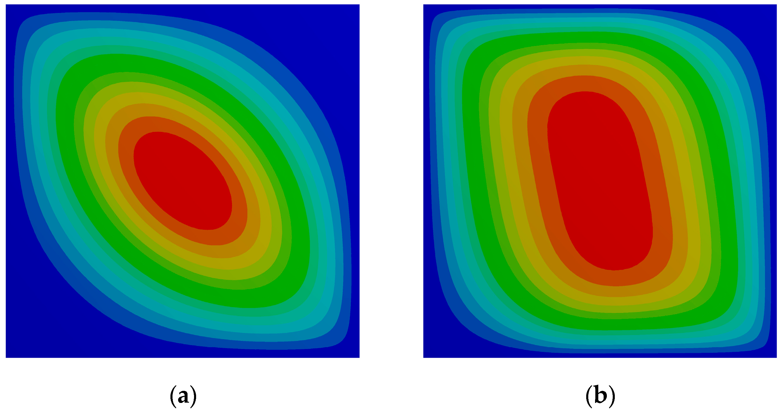
Figure 5 depicts the color gradient contour plot of the optimal solution for the constant stiffness composite (a) and the variable stiffness composite (b) in the case of the simply supported boundary conditions.
As it is possible to observe, in the second case, the shape profile of the deflection surface is more balanced and the color gradient illustrates also the difference between the quantitative values presented in Table 17.
The maximization of the fundamental frequency of the simply supported three-layer composite was addressed next. The results obtained both for a constant stiffness and for a variable stiffness composite are presented in Table 19 and the corresponding mode shapes depicted in Figure 6.
As in the single layer composite previously optimized, it is possible to conclude on the improvement of the maximum frequency of the VS composite plate, although to a less extent. It is also visible from Figure 6 that the vibration mode shape for the optimal configuration VS case acquires a more balanced profile toward biaxial symmetry, quite different from the one presented by the CS composite. It can also be observed that VS plates present in most cases, the outer layers with similar angles. It can also be observed that for the cases analyzed the angles of the outer layers present amplitudes close to the ones corresponding to the single-layer optimal configuration.
This is, with terminology adaptations, applicable to the CS plates, which is an expected result considering the higher contribution that these layers provide to the fundamental frequency that corresponds to a flexural mode.
The final optimization studies are related to the determination of the optimal layups that will provide the maximum critical buckling load multipliers both in uniaxial and biaxial compression load cases. The results obtained can be observed in Table 20 and the corresponding color gradient contour plots are visible in Figure 7 and Figure 8.
From Table 20 it can be concluded again that VS composites can have significant importance in the maximization of the critical buckling load corresponding to a uniaxial compression load case. This was already seen in the context of a single-layer. The aspect related to the magnitude of the angles presented by the outer layers is also here confirmed.
Concerning the corresponding critical mode shape, it can be observed that there is an elongation trend more visible in contrast to the one presented by the constant stiffness composite in the case of the uniaxial compression load. A similar elongation pattern is observed in Figure 8, for the biaxial critical buckling load, although more balanced when compared to the constant stiffness composite plate.
5. Conclusions
Due to their known fiber curvilinear paths, VS composites can provide greater design flexibility when compared to constant stiffness laminates, as they may enable for an eventual adjustment to geometrical specificities, such as holes, and contribute for a better load redistribution. Moreover, the possibility of selecting the better configurations for specific boundary conditions can be a very important feature to improve structures’ mechanical performance while considering functional or manufacturability constraints.
This work presents a study on the optimization of VS composite plates considering the minimization of the maximum transverse deflection, the maximization of the fundamental frequency, and of the critical buckling load both in a uniaxial and biaxial compression load condition.
A set of studies based on first-order shear deformation theory were developed in a preliminary phase of the work for verification purposes and also with the aim of providing a more complete set of analyses namely for the three-layer VS composite, prior to the optimization case studies.
The optimization studies, based on an adaptive hybrid technique, have considered single-layer and three-layer composite plates, having as design variables the characteristic fiber angles, T0 and T1, within each layer. To guarantee manufacturability conditions, according to results obtained by other authors, the present optimization studies took into account that feasibility constraint.
From the results of the single layer case, it can be seen that the VS composite plates present a particularly improved behavior when they are simply supported on all their edges, having the maximum transverse deflection decreased by 14.30%, the fundamental frequency has increased by 8.16%, and the buckling load multipliers has increased by 15.96% and 43.45% for the uniaxial and biaxial load, respectively.
For the three-layer configuration, the VS composite plates also shown significant improvement over the CS composite ones, particularly for the simply supported boundary condition, having the maximum transverse deflection decreased by 11.26%, the frequency increased by 5.61%, and the buckling load multipliers increased by 51.13% and 58.01% for the uniaxial and biaxial load, respectively.
In a global appreciation, VS composite plates present better results when compared to CS composite ones. However, the results obtained allow concluding that in some situations that depend not only on the boundary conditions but also on the nature of the objective function to be assessed, the advantage of the former may be not so significant.
The achieved results provide a transversal overview on the potential advantages of variable stiffness composites, nevertheless for each specific optimization case, eventually ruled by other constraints, other specific studies may be required.
Author Contributions
F.E.C.M.: Data curation, Conceptualization, Methodology, Software, Verification, Writing—original draft. A.F.S.d.M.: Data curation, Writing—original draft. M.A.R.L.: Conceptualization, Methodology, Formal analysis, Supervision, Writing—review & editing, Project administration. All authors have read and agreed to the published version of the manuscript.
Funding
This research was funded by Project IPL/2019/MOCHVar/ISEL and Project IDMEC, LAETA UIDB/50022/2020.
Acknowledgments
The authors wish to acknowledge the support given by Project IPL/2019/MOCHVar/ISEL, and also the support of FCT/MEC through Project IDMEC, LAETA UIDB/50022/2020.
Conflicts of Interest
The authors declare no conflict of interest.
References
- Xu, Y.; Zhu, J.; Wu, Z.; Cao, Y.; Zhao, Y.; Zhang, W. A review on the design of laminated composite structures: Constant and variable stiffness design and topology optimization. Adv. Compos. Hybrid Mater. 2018, 1, 460–477. [Google Scholar] [CrossRef]
- Lozano, G.G.; Tiwari, A.; Turner, C.; Astwood, S. A review on design for manufacture of variable stiffness composite laminates. Proc. Inst. Mech. Eng. Part B J. Eng. Manuf. 2015, 230, 981–992. [Google Scholar] [CrossRef]
- Setoodeh, S.; Gurdal, Z.; Watson, L.T. Design of variable-stiffness composite layers using cellular automata. Comput. Methods Appl. Mech. Eng. 2006, 195, 836–851. (In English) [Google Scholar] [CrossRef]
- Abdalla, M.M.; Setoodeh, S.; Gürdal, Z. Design of variable stiffness composite panels for maximum fundamental frequency using lamination parameters. Compos. Struct. 2007, 81, 283–291. [Google Scholar] [CrossRef]
- Setoodeh, S.; Abdalla, M.M.; Jsselmuiden, S.T.I.; Gürdal, Z. Design of variable-stiffness composite panels for maximum buckling load. Compos. Struct. 2009, 87, 109–117. [Google Scholar] [CrossRef]
- Lopes, C.S.; Gürdal, Z.; Camanho, P.P. Variable-stiffness composite panels: Buckling and first-ply failure improvements over straight-fibre laminates. Comput. Struct. 2008, 86, 897–907. (In English) [Google Scholar] [CrossRef]
- Gürdal, Z.; Tatting, B.F.; Wu, C.K. Variable stiffness composite panels: Effects of stiffness variation on the in-plane and buckling response. Compos. Part A Appl. Sci. Manuf. 2008, 39, 911–922. [Google Scholar] [CrossRef]
- Hao, P.; Yuan, X.; Liu, H.; Wang, B.; Liu, C.; Yang, D.; Zhan, S. Isogeometric buckling analysis of composite variable-stiffness panels. Compos. Struct. 2017, 165, 192–208. [Google Scholar] [CrossRef]
- Honda, S.; Oonishi, Y.; Narita, Y.; Sasaki, K. Vibration Analysis of Composite Rectangular Plates Reinforced along Curved Lines. J. Syst. Des. Dyn. 2008, 2, 76–86. [Google Scholar] [CrossRef] [Green Version]
- Houmat, A. Three-dimensional free vibration analysis of variable stiffness laminated composite rectangular plates. Compos. Struct. 2018, 194, 398–412. [Google Scholar] [CrossRef]
- Akhavan, H.; Ribeiro, P.; de Moura, M.F.S.F. Large deflection and stresses in variable stiffness composite laminates with curvilinear fibres. Int. J. Mech. Sci. 2013, 73, 14–26. [Google Scholar] [CrossRef]
- Venkatachari, A.; Natarajan, S.; Ganapathi, M. Variable stiffness laminated composite shells—Free vibration characteristics based on higher-order structural theory. Compos. Struct. 2018, 188, 407–414. [Google Scholar] [CrossRef]
- Sarvestani, H.Y.; Akbarzadeh, A.H.; Hojjati, M. Hygro-thermo-mechanical analysis of fiber-steered composite conical panels. Compos. Struct. 2017, 179, 146–160. [Google Scholar] [CrossRef]
- Demir, E.; Yousefi-Louyeh, P.; Yildiz, M. Design of variable stiffness composite structures using lamination parameters with fiber steering constraint. Compos. Part B Eng. 2019, 165, 733–746. [Google Scholar] [CrossRef]
- Shafighfard, T.; Demir, E.; Yildiz, M. Design of fiber-reinforced variable-stiffness composites for different open-hole geometries with fiber continuity and curvature constraints. Compos. Struct. 2019, 226, 111280. [Google Scholar] [CrossRef]
- Hao, P.; Liu, D.; Wang, Y.; Liu, X.; Wang, B.; Li, G.; Feng, S. Design of manufacturable fiber path for variable-stiffness panels based on lamination parameters. Compos. Struct. 2019, 219, 158–169. [Google Scholar] [CrossRef]
- Murugan, S.; Flores, E.I.S.; Adhikari, S.; Friswell, M.I. Optimal design of variable fiber spacing composites for morphing aircraft skins. Compos. Struct. 2012, 94, 1626–1633. [Google Scholar] [CrossRef]
- Murugan, S.; Friswell, M.I. Morphing wing flexible skins with curvilinear fiber composites. Compos. Struct. 2013, 99, 69–75. [Google Scholar] [CrossRef]
- Wu, Z.; Weaver, P.M.; Raju, G.; Kim, B.C. Buckling analysis and optimisation of variable angle tow composite plates. Thin-Walled Struct. 2012, 60, 163–172. [Google Scholar] [CrossRef] [Green Version]
- Reddy, J.N. Mechanics of Laminated Composite Plates and Shells: Theory and Analysis, 2nd ed.; CRC Press: Boca Raton, FL, USA, 2004. [Google Scholar]
- Zienkiewicz, O.C.; Taylor, R.L. The Finite Element Method, 5th ed.; Butterworth-Heinemann: Oxford, UK, 2000; Volume 1. [Google Scholar]
- Gürdal, Z.; Olmedo, R. Composite laminates with spatially varying fiber orientations—‘Variable stiffness panel concept’. In Proceedings of the 33rd Structures, Structural Dynamics and Materials Conference, Dallas, TX, USA, 13–15 April 1992. [Google Scholar]
- Waldhart, C.; Gurdal, Z.; Ribbens, C. Analysis of tow placed, parallel fiber, variable stiffness laminates. In Proceedings of the 37th Structure, Structural Dynamics and Materials Conference, Salt Lake City, UT, USA, 15–17 April 1996. [Google Scholar]
- Reissner, E. On the theory of transverse bending of elastic plates. Int. J. Solids Struct. 1976, 12, 545–554. [Google Scholar] [CrossRef]
- Mindlin, R.D. Influence of rotary inertia and shear on flexural motions of isotropic elastic plates. J. Appl. Mech. Asme 1951, 18, 31–38. [Google Scholar]
- Loja, M.A.R.; Barbosa, J.I.; Soares, C.M.M. Dynamic instability of variable stiffness composite plates. Compos. Struct. 2017, 182, 402–411. [Google Scholar] [CrossRef]
- Mota, A.F.; Loja, M.A.R.; Barbosa, J.I.; Rodrigues, J.A. Porous functionally graded plates: An assessment of shear correction factor influence on static behavior. Math. Comput. Appl. 2020, 25, 25. [Google Scholar]
- Moré, J.J.; Wright, S.J. Optimization Software Guide; Frontiers in Applied Mathematics; Society for Industrial and Applied Mathematics: Philadelphia, PA, USA, 1993. [Google Scholar]
- Yang, X.; He, X. Introduction to Optimization; Springer Nature: Basel, Switzerland, 2019. [Google Scholar]
- ANSYS DesignXplorer User’s Guide; ANSYS, Inc.: Fort Williams, PA, USA, 2020.
- Silva, T.A.N.; Loja, M.A.R.; Maia, N.M.M.; Barbosa, J.I. A hybrid procedure to identify the optimal stiffness coefficients of elastically restrained beams. Int. J. Appl. Math. Comput. Sci. 2015, 25, 245–257. [Google Scholar] [CrossRef] [Green Version]
- MathWorks. Available online: https://www.mathworks.com/ (accessed on 23 June 2020).
- Phan, N.D.; Reddy, J.N. Analysis of Laminated Composite Plates Using a Higher-Order Shear Deformation-Theory. Int. J. Numer. Methods Eng. 1985, 21, 2201–2219. [Google Scholar] [CrossRef]
- Akhavan, H.; Ribeiro, P. Natural modes of vibration of variable stiffness composite laminates with curvilinear fibers. Compos. Struct. 2011, 93, 3040–3047. (In English) [Google Scholar] [CrossRef]
Figure 1.
Fiber Path for 〈20|60〉 configuration (left) and 〈50|−20〉 configuration (right).

Figure 2.
Feasible manufacturing fiber angles domain, in white.

Figure 3.
Angles discretization. (a) 10 × 10 mesh, (b) 50 × 50 mesh.
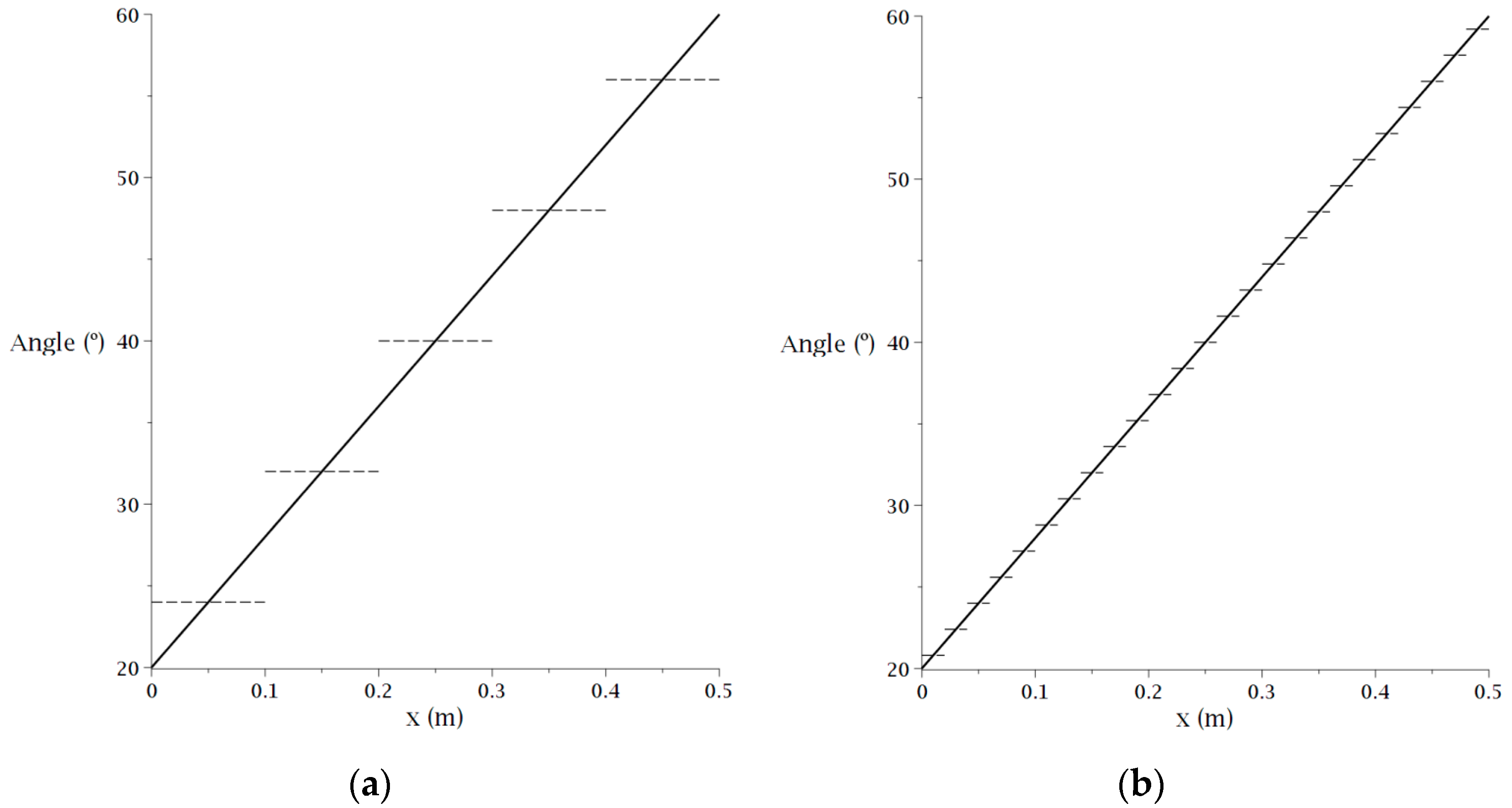
Figure 4.
Contour plots. (a) buckling uniaxial, (b) buckling biaxial, and (c) frequency.
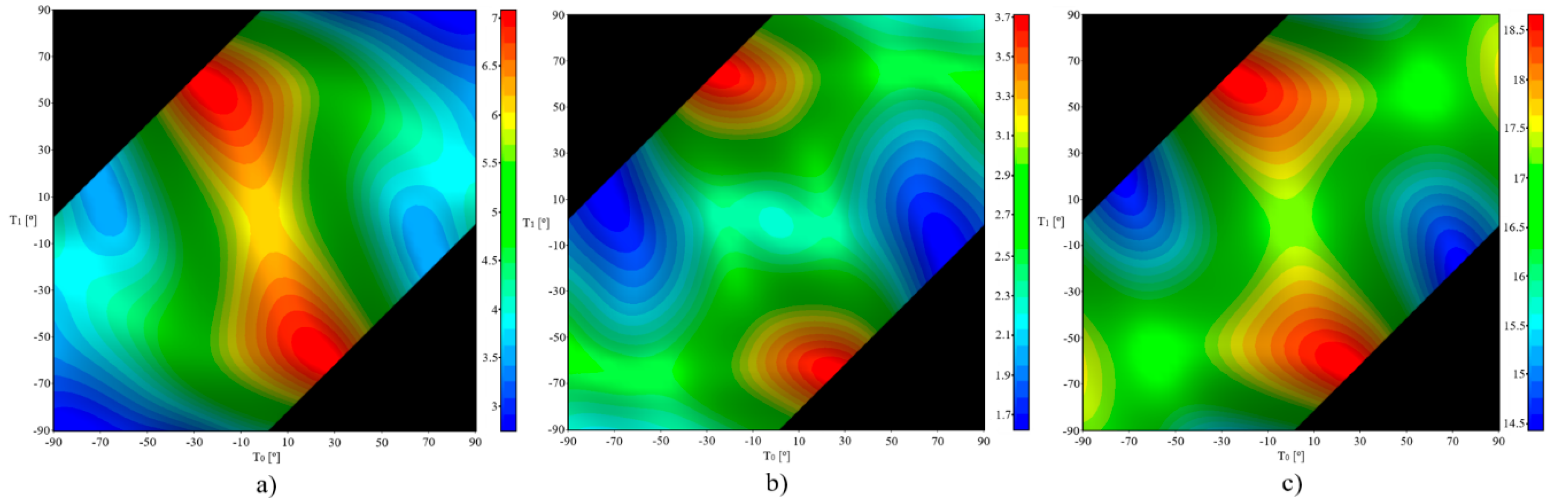
Figure 5.
Transverse deflection surface for the optimal layups for the SSSS case. (a) constant stiffness (CS) and (b) VS.
Figure 5.
Transverse deflection surface for the optimal layups for the SSSS case. (a) constant stiffness (CS) and (b) VS.

Figure 6.
Fundamental vibration mode shape for the optimal layups for the SSSS plate. (a) CS and (b) VS.
Figure 6.
Fundamental vibration mode shape for the optimal layups for the SSSS plate. (a) CS and (b) VS.

Figure 7.
Critical buckling mode shape for the optimal layups for the SSSS plate. (a) CS and (b) VS uniaxial buckling.
Figure 7.
Critical buckling mode shape for the optimal layups for the SSSS plate. (a) CS and (b) VS uniaxial buckling.

Figure 8.
Critical buckling mode shape for the optimal layups for the SSSS plate. (a) CS and (b) VS biaxial buckling.
Figure 8.
Critical buckling mode shape for the optimal layups for the SSSS plate. (a) CS and (b) VS biaxial buckling.

Table 1.
Non-dimensional frequencies for α = 1.0.
| Mode | SSSS | CCCC | SFSF | CFCF | ||||
|---|---|---|---|---|---|---|---|---|
| CLPT | FSDT | CLPT | FSDT | CLPT | FSDT | CLPT | FSDT | |
| 1 | 19.737 (0.010) | 19.739 | 35.975 (0.031) | 36.006 | 3.367 (0.089) | 3.367 | 6.920 (0.058) | 6.923 |
| 2 | 49.337 (0.022) | 49.350 | 73.364 (0.042) | 73.483 | 17.318 (0.046) | 17.316 | 23.908 (0.063) | 23.914 |
| 3 | 49.337 (0.022) | 49.350 | 73.364 (0.042) | 73.483 | 19.293 (0.078) | 19.293 | 26.584 (0.026) | 26.590 |
| 4 | 78.922 (0.044) | 78.959 | 108.127 (0.084) | 108.629 | 38.214 (0.196) | 38.211 | 47.655 (0.031) | 47.675 |
| 5 | 98.666 (0.642) | 98.695 | 131.508 (0.206) | 131.755 | 51.044 (0.513) | 51.036 | 62.710 (0.223) | 62.718 |
| 6 | 98.666 (0.642) | 98.695 | 132.138 (0.205) | 132.471 | 53.492 (0.705) | 53.488 | 65.536 (0.227) | 65.557 |
Table 2.
Non-dimensional frequencies for α = 2.5.
| Mode | SSSS | CCCC | SFSF | CFCF | ||||
|---|---|---|---|---|---|---|---|---|
| CLPT | FSDT | CLPT | FSDT | CLPT | FSDT | CLPT | FSDT | |
| 1 | 71.552 (0.004) | 71.585 | 147.757 | 147.939 | 8.247 (0.243) | 8.247 | 24.830 (0.068) | 24.831 |
| 2 | 101.154 (0.010) | 101.202 | 173.758 | 173.957 | 29.568 (0.125) | 29.571 | 44.562 (0.079) | 44.565 |
| 3 | 150.490 (0.333) | 150.595 | 221.295 | 221.568 | 64.478 (0.820) | 64.492 | 81.496 (0.214) | 81.519 |
| 4 | 219.559 (1.530) | 219.812 | 291.595 | 292.084 | 98.684 (0.154) | 98.737 | 135.810 (1.769) | 135.910 |
| 5 | 256.587 (0.009) | 257.093 | 384.200 | 385.100 | 117.791 (2.473) | 117.857 | 142.475 (3.188) | 142.607 |
| 6 | 286.171 (0.017) | 286.711 | 394.201 | 395.538 | 125.624 (0.705) | 125.690 | 165.002 (0.236) | 165.144 |
Table 3.
Non-dimensional buckling coefficient .
| E1/E2 | Present FSDT | HSDT | |
|---|---|---|---|
| k Calculated | k = 5/6 | [33] | |
| 10 | 10.061 (2.936) | 10.076 (3.090) | 9.774 |
| 20 | 15.606 (2.013) | 15.633 (2.190) | 15.298 |
| 30 | 20.186 (1.147) | 20.235 (1.393) | 19.957 |
| 40 | 24.045 (3.021) | 24.131 (3.389) | 23.34 |
Table 4.
Geometric and material characteristics of the plate.
| a (m) | h (m) | E1 (GPa) | E2 (GPa) | G12 (GPa) | ν12 | ρ (kg·m−1) |
|---|---|---|---|---|---|---|
| 1 | 0.01 | 173 | 7.2 | 3.76 | 0.29 | 1540 |
Table 5.
Natural frequencies (rads·s−1).
| Stacking | Models | ω (rad·s−1) | |||||
|---|---|---|---|---|---|---|---|
| 1 | 2 | 3 | 4 | 5 | 6 | ||
| (<0|45>, <−45|−60>, <0|45>) | Present | 355.30 | 586.66 | 958.69 | 1070.28 | 1317.52 | 1464.42 |
| [26] | 347.1 (2.36) | 576.1 (1.83) | 949.31 (0.99) | 1066.64 (0.34) | 1300.47 (1.31) | 1457.21 (0.50) | |
| [34] | 358.49 (0.89) | 589.9 (0.55) | 960.36 (0.17) | 1075.21 (0.46) | 1327.88 (0.78) | 1474.67 (0.70) | |
| (<30|0>, <45|90>, <30|0>) | Present | 308.66 | 503.63 | 845.09 | 1130.41 | 1276.93 | 1305.21 |
| [26] | 308.03 (0.20) | 502.03 (0.32) | 842.79 (0.27) | 1133.79 (0.30) | 1277.26 (0.03) | 1300.73 (0.34) | |
| [34] | 308.8 (0.05) | 503.8 (0.03) | 845.51 (0.05) | 1131.31 (0.08) | 1279.85 (0.23) | 1307.4 (0.17) | |
| (<90|45>, <60|30>, <90|45>) | Present | 326.20 | 533.07 | 880.53 | 1082.91 | 1259.90 | 1388.02 |
| [26] | 320.05 (1.92) | 521.15 (2.29) | 877.23 (0.38) | 1084.42 (0.14) | 1238.85 (1.70) | 1395.8 (0.56) | |
| [34] | 329.69 (1.06) | 539.41 (1.18) | 886.39 (0.66) | 1091.2 (0.76) | 1279.9 (1.56) | 1401.87 (0.99) | |
Table 6.
Magnitudes of the uniformly distributed pressure.
| Layers | Boundary Condition | ||||||
|---|---|---|---|---|---|---|---|
| SSSS | CCCC | SSFF | CCFF | SFSF | CFCF | ||
| Pressure (kPa) | 1 | 1 | 1 | 0.1 | 0.1 | 0.01 | 0.1 |
| 3 | 10 | 10 | 1 | 1 | 0.1 | 1 | |
Table 7.
Maximum transverse deflection [mm] for the three-layer configurations of variable stiffness (VS) plates.
Table 7.
Maximum transverse deflection [mm] for the three-layer configurations of variable stiffness (VS) plates.
| Stacking | Boundary Condition | |||||
|---|---|---|---|---|---|---|
| SSSS | CCCC | SSFF | CCFF | SFSF | CFCF | |
| (<0|45>, <−45|−60>, <0|45>) | 7.894 | 3.005 | 1.456 | 0.411 | 8.571 | 10.834 |
| (<30|0>, <45|90>, <30|0>) | 10.83 | 2.285 | 2.167 | 0.339 | 15.657 | 7.100 |
| (<90|45>, <60|30>, <90|45>) | 9.736 | 2.016 | 18.951 | 1.938 | 10.382 | 9.388 |
Table 8.
Buckling load multipliers for the three-layer configurations of VS plates.
| Stacking | Loading | 1 | 2 | 3 | 4 | 5 | 6 |
|---|---|---|---|---|---|---|---|
| (<0|45>, <−45|−60>, <0|45>) | Uniaxial | 2.12 | 3.865 | 5.519 | 6.625 | 7.337 | 8.122 |
| Biaxial | 1.091 | 1.208 | 1.678 | 2.384 | 3.08 | 3.203 | |
| (<30|0>, <45|90>, <30|0>) | Uniaxial | 1.451 | 3.091 | 4.765 | 5.651 | 6.895 | 7.987 |
| Biaxial | 0.794 | 0.831 | 1.218 | 1.742 | 2.327 | 2.880 | |
| (<90|45>, <60|30>, <90|45>) | Uniaxial | 1.006 | 1.132 | 1.674 | 1.937 | 2.684 | 3.153 |
| Biaxial | 0.658 | 0.750 | 1.148 | 1.585 | 2.083 | 2.295 |
Table 9.
Optimum angles for a single layer VS plate for SSSS, SSFF, and SFSF boundary conditions.
| Properties | SSSS | SSFF | SFSF | |||
|---|---|---|---|---|---|---|
| CS | VS | CS | VS | CS | VS | |
| T0 (°) | 0 | 19.124 | 0 | 0.005 | −45 | −41.002 |
| T1 (°) | 0 | −62.531 | 0 | 0.017 | −45 | −50.329 |
| (mm) | 25.118 | 21.526 | 2.540 | 2.540 | 11.963 | 11.843 |
| Decrease (%) | - | 14.301 | - | 0 | - | 1.003 |
Table 10.
Optimum angles for a single layer VS plate for CCCC, CCFF, and CFCF boundary conditions.
| Properties | CCCC | CCFF | CFCF | |||
|---|---|---|---|---|---|---|
| CS | VS | CS | VS | CS | VS | |
| T0 (°) | 0 | 0.015 | 0 | 0.000 | 78.174 | 30.998 |
| T1 (°) | 0 | −0.004 | 0 | −0.001 | 78.174 | −1.155 |
| (mm) | 5.109 | 5.109 | 0.501 | 0.501 | 20.101 | 19.193 |
| Decrease (%) | - | 0 | - | 0 | - | 4.517 |
Table 11.
Optimal angles of a single layer VS plate for maximum fundamental frequency (Hz), with simply supported boundary conditions.
Table 11.
Optimal angles of a single layer VS plate for maximum fundamental frequency (Hz), with simply supported boundary conditions.
| Properties | SSSS | SSFF | SFSF | |||
|---|---|---|---|---|---|---|
| CS | VS | CS | VS | CS | VS | |
| T0 (°) | 0 | 22.828 | 0 | 0 | −45 | −40.493 |
| T1 (°) | 0 | −62.043 | 0 | 0 | −45 | −51.166 |
| (Hz) | 17.224 | 18.630 | 16.032 | 16.032 | 2.932 | 2.950 |
| Increase (%) | - | 8.164 | - | 0 | - | 0.614 |
Table 12.
Optimal angles of a single layer VS plate for maximum fundamental frequency (Hz), with clamped boundary conditions.
Table 12.
Optimal angles of a single layer VS plate for maximum fundamental frequency (Hz), with clamped boundary conditions.
| Properties | CCCC | CCFF | CFCF | |||
|---|---|---|---|---|---|---|
| CS | VS | CS | VS | CS | VS | |
| T0 (°) | 0 | −90 | 0 | 0 | 76.852 | −40.493 |
| T1 (°) | 0 | −1.680 | 0 | 0 | 76.852 | −51.166 |
| (Hz) | 37.664 | 39.498 | 36.324 | 36.324 | 6.671 | 2.950 |
| Increase (%) | - | 4.869 | - | 0 | - | 4.062 |
Table 13.
Optimal angles of a single layer VS plate for maximum uniaxial load multipliers, with simply supported boundary conditions.
Table 13.
Optimal angles of a single layer VS plate for maximum uniaxial load multipliers, with simply supported boundary conditions.
| Properties | SSSS | SSFF | SFSF | |||
|---|---|---|---|---|---|---|
| CS | VS | CS | VS | CS | VS | |
| T0 (°) | 0 | 23.057 | 0 | 0 | 43.256 | 34.701 |
| T1 (°) | 0 | −57.401 | 0 | 0 | 43.256 | 49.791 |
| 6.091 | 7.063 | 5.278 | 5.278 | 0.319 | 0.325 | |
| Increase (%) | - | 15.958 | - | 0 | - | 1.881 |
Table 14.
Optimal angles of a single layer VS plate for maximum uniaxial load multipliers, with clamped boundary conditions.
Table 14.
Optimal angles of a single layer VS plate for maximum uniaxial load multipliers, with clamped boundary conditions.
| Properties | CCCC | CCFF | CFCF | |||
|---|---|---|---|---|---|---|
| CS | VS | CS | VS | CS | VS | |
| T0 (°) | 0 | 0 | 0 | 0 | 12.386 | 15.750 |
| T1 (°) | 0 | 0 | 0 | 0 | 12.386 | 7.048 |
| 22.672 | 22.672 | 21.098 | 21.098 | 1.881 | 1.891 | |
| Increase (%) | - | 0 | - | 0 | - | 1.891 |
Table 15.
Optimal angles of a single layer VS plate for maximum biaxial load multipliers, with simply supported boundary conditions.
Table 15.
Optimal angles of a single layer VS plate for maximum biaxial load multipliers, with simply supported boundary conditions.
| Properties | SSSS | SSFF | SFSF | |||
|---|---|---|---|---|---|---|
| CS | VS | CS | VS | CS | VS | |
| T0 (°) | 69.748 | 27.047 | 0 | 0 | −45 | −43.145 |
| T1 (°) | 69.748 | −66.919 | 0 | 0 | −45 | −47.282 |
| 2.594 | 3.721 | 1.331 | 1.331 | 0.175 | 0.175 | |
| Increase (%) | - | 43.448 | - | 0 | - | 0 |
Table 16.
Optimal angles of a single layer VS plate for maximum biaxial load multipliers, with clamped boundary conditions.
Table 16.
Optimal angles of a single layer VS plate for maximum biaxial load multipliers, with clamped boundary conditions.
| Properties | CCCC | CCFF | CFCF | |||
|---|---|---|---|---|---|---|
| CS | VS | CS | VS | CS | VS | |
| T0 (°) | 0 | 10.852 | 16.874 | 79.914 | 45 | 60.389 |
| T1 (°) | 0 | −83.098 | 16.874 | −14.036 | 45 | 39.411 |
| 5.699 | 6.659 | 2.890 | 3.626 | 0.987 | 1.033 | |
| Increase (%) | - | 16.845 | - | 25.467 | - | 4.661 |
Table 17.
Optimum angles for a three-layer VS plate minimum, maximum transverse deflection. SSSS, SSFF, and SFSF boundary conditions.
Table 17.
Optimum angles for a three-layer VS plate minimum, maximum transverse deflection. SSSS, SSFF, and SFSF boundary conditions.
| Layer | Properties | SSSS | SSFF | SFSF | |||
|---|---|---|---|---|---|---|---|
| CS | VS | CS | VS | CS | VS | ||
| 1 | T0 (°) | −45 | −25.008 | 0 | 0 | 45 | 47.528 |
| T1 (°) | −45 | 62.886 | 0 | 0 | 45 | 42.625 | |
| 2 | T0 (°) | 45 | 26.499 | 0 | 0 | 45 | 49.833 |
| T1 (°) | 45 | 41.007 | 0 | 0 | 45 | 40.039 | |
| 3 | T0 (°) | −45 | −15.557 | 0 | 0 | −45 | −42.512 |
| T1 (°) | −45 | −54.835 | 0 | 0 | −45 | −47.796 | |
| (mm) | 8.529 | 7.569 | 0.945 | 0.945 | 2.718 | 2.704 | |
| Decrease (%) | - | 11.2578 | - | 0 | - | 0.515123 | |
Table 18.
Optimum angles for a three-layer VS plate minimum, maximum transverse deflection. CCCC, CCFF, and CFCF boundary conditions.
Table 18.
Optimum angles for a three-layer VS plate minimum, maximum transverse deflection. CCCC, CCFF, and CFCF boundary conditions.
| Layer | Properties | CCCC | CCFF | CFCF | |||
|---|---|---|---|---|---|---|---|
| CS | VS | CS | VS | CS | VS | ||
| 1 | T0 (°) | 0 | 90 | 0 | 0 | 12.422 | 36.051 |
| T1 (°) | 0 | 90 | 0 | 0 | 12.422 | 0.913 | |
| 2 | T0 (°) | 0 | −90 | 0 | 0 | 46.505 | −70.004 |
| T1 (°) | 0 | −90 | 0 | 0 | 46.505 | −35.080 | |
| 3 | T0 (°) | 0 | 90 | 0 | 0 | 12.419 | 36.047 |
| T1 (°) | 0 | 90 | 0 | 0 | 12.419 | 0.917 | |
| (mm) | 1.930 | 1.930 | 0.189 | 0.189 | 7.458 | 6.667 | |
| Decrease (%) | - | 0 | - | 0 | - | 10.605 | |
Table 19.
Optimum angles for the maximum fundamental frequency [Hz] of a three-layer variable stiffness composite plate.
Table 19.
Optimum angles for the maximum fundamental frequency [Hz] of a three-layer variable stiffness composite plate.
| Layer | Properties | Fundamental Frequency | |
|---|---|---|---|
| CS | VS | ||
| 1 | T0 (°) | −45 | 16.715 |
| T1 (°) | −45 | −60.572 | |
| 2 | T0 (°) | 45 | 57.990 |
| T1 (°) | 45 | 38.114 | |
| 3 | T0 (°) | −45 | 16.720 |
| T1 (°) | −45 | −60.573 | |
| (Hz) | 54.937 | 58.016 | |
| Increase (%) | - | 5.605 | |
Table 20.
Optimal angles of a three-layer VS plate for static buckling load multipliers.
| Layer | Properties | Uniaxial Buckling | Biaxial Buckling | ||
|---|---|---|---|---|---|
| CS | VS | CS | VS | ||
| 1 | T0 (°) | −6.925 | 30.476 | −45 | 23.369 |
| T1 (°) | −6.925 | −59.626 | −45 | −62.232 | |
| 2 | T0 (°) | 41.121 | 71.359 | 45 | −19.928 |
| T1 (°) | 41.121 | 41.604 | 45 | 73.375 | |
| 3 | T0 (°) | −6.925 | 30.473 | −45 | 23.355 |
| T1 (°) | −6.925 | −59.626 | −45 | −62.236 | |
| 1.698 | 2.565 | 0.818 | 1.293 | ||
| Increase (%) | - | 51.128 | - | 58.005 | |
© 2020 by the authors. Licensee MDPI, Basel, Switzerland. This article is an open access article distributed under the terms and conditions of the Creative Commons Attribution (CC BY) license (http://creativecommons.org/licenses/by/4.0/).
Share and Cite
MDPI and ACS Style
Marques, F.E.C.; Mota, A.F.S.d.; Loja, M.A.R. Variable Stiffness Composites: Optimal Design Studies. J. Compos. Sci. 2020, 4, 80. https://doi.org/10.3390/jcs4020080
AMA Style
Marques FEC, Mota AFSd, Loja MAR. Variable Stiffness Composites: Optimal Design Studies. Journal of Composites Science. 2020; 4(2):80. https://doi.org/10.3390/jcs4020080
Chicago/Turabian StyleMarques, Filipe Eduardo Correia, Ana Filipa Santos da Mota, and Maria Amélia Ramos Loja. 2020. "Variable Stiffness Composites: Optimal Design Studies" Journal of Composites Science 4, no. 2: 80. https://doi.org/10.3390/jcs4020080