
Numerical Model for a Geometrically Nonlinear Analysis of Beams with Composite Cross-Sections

Department of Engineering Mechanics, Faculty of Engineering, University of Rijeka, 51000 Rijeka, Croatia
*
Author to whom correspondence should be addressed.
J. Compos. Sci. 2022, 6(12), 377; https://doi.org/10.3390/jcs6120377
Submission received: 3 November 2022
/
Revised: 16 November 2022
/
Accepted: 2 December 2022
/
Published: 7 December 2022
(This article belongs to the Special Issue Feature Papers in Journal of Composites Science in 2022)
Abstract
:This paper presents a beam model for a geometrically nonlinear stability analysis of the composite beam-type structures. Each wall of the cross-section can be modeled with a different material. The nonlinear incremental procedure is based on an updated Lagrangian formulation where in each increment, the equilibrium equations are derived from the virtual work principle. The beam model accounts for the restrained warping and large rotation effects by including the nonlinear displacement field of the composite cross-section. First-order shear deformation theories for torsion and bending are included in the model through Timoshenko’s bending theory and a modified Vlasov’s torsion theory. The shear deformation coupling effects are included in the model using the six shear correction factors. The accuracy and reliability of the proposed numerical model are verified through a comparison of the shear-rigid and shear-deformable beam models in buckling problems. The obtained results indicated the importance of including the shear deformation effects at shorter beams and columns in which the difference that occurs is more than 10 percent.
1. Introduction
Due to their appealing characteristics, composites have occupied a considerable place in the design process of load-bearing structures. Weight, load-bearing capacity, functionality, construction cost, energy efficiency, and resistance to the chemical processes are some of the characteristics now able to be optimized by the use of different composite materials [1,2,3], including the currently widely applied FRP composites [4,5,6,7].
Furthermore, thin-walled structures provide additional possibilities for optimizing structures in some of the above-mentioned elements. Although there is a wider area for the optimization of such structures, the response of such a structure to the effects of external loading is much more complex. It should be emphasized that there is a tendency of such a structure to lose the stability of the deformation form and the appearance of the buckling [8,9]. Therefore, to produce optimal design solutions for such structures, an exact determination of the limit state of the stability of the deformation forms, or of the buckling strength, is of the utmost interest [10,11,12]. We note that the analytical solutions of such complex structures are limited to only simple cases and primarily deal with just one beam/column [13,14,15], and the development of an accurate numerical model is imposed as a necessity [11,12].
Although for slender beam-type structural members, shear deformations do not play a critical role in the determination of the buckling limit state and, respectively, the Euler-Bernoulli and Vlasov theories for bending and torsion could be applied [16,17], a combination of composite materials and various external loading conditions can provide more pronounced shear deformations [18,19,20]. Several geometric nonlinear analyses of composite beam structures with the influence of shear deformations are presented in [10,11,12]. It should be emphasized here that these numerical models include higher numbers of degrees of freedom over the cross-section area, resulting in accurate models capable of dealing with local stability issues, but they are very computationally demanding and, thus, are hardly applicable for frame-type structures. In order to simplify the numerical models and include the shear deformation effects applicable for frame structures, some researchers have applied more conventional beam models [21,22,23,24,25]. For asymmetric thin-walled cross-sections at which the principal bending and shear axes do not coincide, bending–torsion coupling effects arise and are more significant in stability strength [21,22,23,24,25,26].
In [27], composite frames were considered where a geometrically nonlinear beam model and shear deformation effects were presented. Cross-section walls were modeled by cross-ply laminates, and the material was same in each wall of the cross-section. As an extension to that work, an improved beam formulation will be presented herein which takes into account a change in material along the walls of a thin-walled cross-section. The material is assumed to be constant along the thickness of the cross-section wall, but it can be different for each wall. Since the coupling between the normal and shear stresses is not considered, the current beam model is not applicable for angle-ply composites. This will be a topic in our future research activities.
The presented beam model also includes the following assumptions: the cross-section is not deformable in its own plane and the beam member is prismatic and straight, while the external loads are conservative and static, the material obeys Hooke’s law, translations and rotations are allowed to be large but strains are treated as small, and the shear coupling effects are introduced through corresponding shear correction factors [21,22,25,27,28].
The element geometric stiffness is obtained using the nonlinear displacement field of a cross-section. The numerical procedure is formulated in the framework of an updated Lagrangian (UL) formulation [17,29]. To describe large rotations, the nonlinear displacement field includes the second-order displacement terms. To preserve the equilibrium conditions at the frame joint, the internal bending and torsion moments are described as semi-tangential [30,31]. The shear locking [32] does not occur in the beam model due to the interdependent shape functions for the deflections and their slopes and for the twist rotations and the warping parameters. The generalized displacement control method is used in the incremental-iteration algorithm [31]. To update the nodal orientations, special transformations are used due to the semi-tangential description of the internal moments [33,34].
2. Kinematics of the Beam Element
A straight beam element with an arbitrary open thin-walled composite cross-section is presented in Figure 1. The coordinate x- and y-axes are the principal inertial axes of the cross-section, while the longitudinal z-axis passes through the centroid O of each cross-section. The shear center S of the cross-section is defined by the coordinates xs and ys. All the cross-section properties are material-weighted.
Displacement increments are described by the rigid-body translations of the cross-sections wO, uS, and vS, and by the rigid-body rotations of the cross-sections φz, φx, and φy. θ is the warping parameter. The displacement field of the cross-section is defined as follows:
where
As can be seen, the displacement field contains nonlinear terms arising from the large rotation effects [35]. The associated Green–Lagrange strain tensor can be written as:
where
It should be noted that the strain increments εx, εy, and γxy in Equation (4) are equal to zero due to the applied beam theories. Since the shear deformation effects are considered, it is valid for the linearized shear strain increments [25]:
where the right superscript ‘SD’ denotes the quantities arising from the shear deformability.
3. Cross-Section Properties
In Figure 1b, an arbitrary open cross-section composed of a number of thin walls is shown. Each wall is composed of a single orthotropic ply, and denote the reference axes, and and are the centroid axes while x and y are the principal ones. Furthermore, s and n are the contour and thickness coordinates with their origins in Oω while R1 is the total number of walls. The incremental constitutive equations valid for a cross-section wall can be written as:
In Equation (6), and denote the transformed reduced stiffness coefficients [36,37], is the linearized normal strain increment, and is the linearized shear strain increment due the St. Venant torsion and is the linearized shear strain increment occurring at bending with shear and warping torsion, respectively [28,38], while Ω denotes the principal warping function. The reference moduli can be determined as follows:
In Figure 2, the local axes (s, n) of each wall should be transformed to the coordinate system of reference axes (, ) of the cross-section as:
In the figure, A is an arbitrary point while R denotes the referent point placed on the centerline on the arbitrary position along the wall (i). Applying Equation (8), the modulus-weighted cross-section area and the modulus-weighted first moments of the area can be obtained as follows:
The coordinates of the centroid with reference to the reference axes of the cross-section can be obtained as:
After the position of the cross-section centroid is determined, the cross-section axes are repositioned to the centroid. All the above cross-sectional properties need to be recalculated for the new position of the axes. Analogously, the modulus-weighted second moments of area can be derived as:
After that, the angles of the principal axes can be obtained from the well-known formula:
Establishing the angle from Equation (12), the cross-section properties should be recalculated for the principal axes of the cross-section.
The warping function is defined for the pole set at the centroid of the cross-section and the associated origin is set according to Figure 1b. From Figure 2b, the difference in contour warping function can be calculated as:
while, from Figure 2c, the difference in thickness warping function is:
By combining Equations (13) and (14), the expression for the warping function of an arbitrary point A is derived as:
The warping function from Equation (15) is used to derive, respectively, the modulus-weighted first and second sectorial moments as:
and afterwards, the shear center position coordinates with reference to the principal axes can be calculated as:
Knowing the position of the shear center, the principal warping function is derived by the following transformation [26]:
and the modulus-weighted warping constant can be determined as:
4. Governing Equations
Applying the conventional engineering theories for torsion and bending, the stress resultant increments, shown in Figure 1a, can be calculated as follows:
where Fz is the axial force, Fx and Fy are the shear forces, TSV is the St. Venant torsion moment, Tω is the warping torsion moment, Mx and My are the bending moments, Mω is the bimoment, and is the Wagner coefficient [17,38]. For a thin-walled composite cross-section, the St. Venant torsion moment can be calculates as [38]:
where is the modulus-weighted torsional moment of inertia, and it is defined as:
From Equations (4), (6), and (20), expressions for the axial force, the bending moments, and the bimoment for a thin-walled composite cross-section can be derived as follows:
where , , , and are the generalized deformation increments.
Since the following is valid tor the principal cross-sectional axes and the principal warping function:
the generalized deformation increments from Equations (29)–(32) can be rewritten as:
while, for the normal stress increment, one can obtain:
Since the shear stress increment is uniformly distributed over a wall thickness, it can be expressed as:
where , , and are, respectively, the modulus-weighted first moments of the area and the first sectorial moment for the cross-section cut off.
The virtual incremental strain energy due to shear deformability is derived using Equations (6) and (27) as follows:
i.e.,
In Equation (29), , , , , , and denote the shear correction factors calculated as:
By using Equations (5) and (6) in Equation (20), the shear forces and the warping torsion moment increments can be expressed in terms of the linearized shear strain increments:
where
In Equation (32), kij and Kij are dimensionless constants, while the explicit solutions of the integrals from Equation (30) are provided in Appendix A.
5. Finite Element Formulation
A thin-walled beam element, as shown in Figure 1, consists of two nodes, and each node has seven degrees-of-freedom. The corresponding nodal displacement and force vectors are:
where the right superscript e denotes the e-th finite element. The virtual work principle for a beam element deforming between the last calculated configuration C1 and the current unknown configuration C2 can be expressed as follows:
where, respectively, the virtual incremental elastic strain and geometric energy are determined as:
In Equation (35), the quantities on the right-hand side represent the virtual incremental work performed by the nodal forces, i.e.,
In the above equations, S is the second Piola–Kirchhoff stress tensor, tn represents the surface tractions, and C is the incremental constitutive tensor. According to the applied UL incremental description, all the quantities occurring in Equations (36)–(39) are expressed with reference to the configuration C1. The index notation adopted in the presented work is the same as that in [31], i.e., the left superscript refers to the configuration in which a quantity occurs while the left subscript refers to the configuration in which the quantity is measured.
Furthermore, the virtual incremental elastic strain energy can be decomposed as:
where the first term on the right-hand side denotes the incremental energy obtained by the Euler–Bernoulli and St. Venant beam theories for bending and torsion, respectively, i.e.,
while the second energy term is due to the shear deformability which, according to Equations (29) and (31), can be defined as:
Applying a linear interpolation for the axial displacement and a cubic interpolation for the deflections and twist rotations, respectively, the rigid-body displacements of the cross-section can be defined as:
where the shape-functions occurring in the first matrix on the right-hand side of Equation (43) are provided in Appendix B. Substituting Equations (36)–(43) into Equation (35), the incremental equilibrium equations for the beam element in C2 can be rewritten as:
where is the incremental elastic stiffness matrix of the beam element while is the corresponding incremental geometric stiffness matrix. To perform the force recovery, the so-called conventional approach [39] is adopted in this work, i.e.,
where denotes the incremental transformation matrix reported in [18]. After performing the assembly procedure, the incremental equilibrium of a beam-type structure can be obtained as:
where 1KE is the incremental elastic stiffness matrix, 1KG is the incremental geometric stiffness matrix, U is the incremental displacement vector, 1P is the external load vector applied on the structure at C1, 2P is the external load vector applied on the structure at C2, and 1te is the transformation matrix for the e-th beam element from the local coordinate system (1z, 1x, and 1y) in C1 to the global coordinate system (Z, X, and Y).
6. Numerical Examples
A computer program, named THINWALL v.17 [25], is developed on the basis of the numerical procedures presented in this paper. The nonlinear stability analysis is performed in the form of incremental-iterative solver based on the generalized control method [31]. To initiate the buckling, a small perturbation load should be introduced. Nodal coordinates and orientations of the cross-section axes of each beam element are updated at the end of each load step [25]. To stop the iteration, energy criteria is adopted with the tolerance value of 10−6.
Three beam models are considered in the analysis in order to emphasize the significance of the shear effects on the stability behavior of the structure under consideration. In the first beam model, the shear deformability effects are ignored entirely, and in the presented results, it is labelled with ‘SR’. The second beam model includes shear deformation coupling effects, using the procedures presented in this paper, and it is labelled with ‘SD’. The last beam model ignores the shear deformation coupling effects, and in the provided diagrams and tables, it is denoted by ‘SD1’. The structural material used in all the examples is graphite-epoxy (AS4/3501), with E1 = 144 GPa, E2 = 9.65 GPa, G12 = 4.14 GPa, and v12 = 0.3, as reported in [11]. The general cross-section shape used in the examples is shown in Figure 3. Each wall of the cross-section is of the same thickness t and is composed of single AS4/3501 ply. The ply orientations are provided in Figure 3.
6.1. Example 1
Figure 4a shows a cantilever column under an axial force F. A mono-symmetric cross-section of 6 × 10 × 6 × 1 cm (b1 × h × b2 × t) is adopted with the properties provided in Table 1. A force F is applied at the geometric centroid of the cross-section. Since the neutral axis passes through the material-weighted centroid, the force acting through the geometric centroid behaves as the off-axis load. The lowest buckling load pertains to the torsional-flexural (TF) mode, as shown in Figure 4c. The second buckling mode is the flexural (F) mode, as shown in Figure 4b. Both modes are analyzed using five different mesh configurations, each consisting of one, two, four, eight, and sixteen beam elements. The results obtained are shown in Figure 5a and are compared with the NX Nastran’s laminate shell results.
As one can see, the shear locking does not occur in any of the shear deformable models and the SD model’s results approach the shell solution. The results obtained by the SD1 model underestimate the column buckling strength in TF mode, leaving the construction on the safe side if shear deformation effects are ignored. Since the beam model assumes a rigid cross-section and is unable to model the cross-section distortion, some differences between the beam model and the shell model are expected for higher loads and shorter beams where the cross-section distortion affects the critical load, as can be observed in the F mode results. Furthermore, the buckling strength reductions due to the shear deformability are 8% and 12% in comparison with the shear rigid model for the TF and F modes, respectively. The buckling strength increase due to the shear coupling effects is 6% for the TF mode, and there is no influence of the shear couplings for the F mode. In Figure 5b, the variations in the value of buckling load against the column slenderness ratio are shown. It can be seen that the differences between the results obtained by the SR and SD beam models are decreasing as the slenderness ratio increases.
6.2. Example 2
In this example, a cantilever beam from Figure 6a is considered. The lateral force F is acting at the free end in the Y-direction through the shear center of the asymmetric cross-section 4 × 10 × 2 × 1 cm. The cross-section properties are shown in Table 2.
Four different mesh configurations, each consisting of two, four, eight, and sixteen beam elements, are used to analyze the lateral-torsional buckling mode in Figure 6b. Since the cross-section is asymmetric, a difference in the buckling load for the positive and negative direction of the force is expected [38]. To initiate the buckling, a small perturbation force of intensity 0.001 F, acting through the shear center in the X-direction, is applied at the free end of the beam.
In Figure 7, the load-deflection curves are presented for the mesh configuration of the sixteen beam elements and for both of the force directions. The convergence study is shown in Figure 8. The critical forces obtained by NX Nastran’s laminate shell model are Fcr = 5.75 kN for the force acting in the +Y direction and Fcr = 13.873 kN for the force acting in the −Y direction. From the figures, it can be seen that all the mesh models recognize the buckling load. Significant differences appear in the post-buckling range above F > 3Fcr and F > 2.5Fcr, respectively. As can be seen, the reductions in the buckling strength due to the shear deformability are 2% and 8% for the positive and negative force directions, respectively.
6.3. Example 3
In this example, an L-frame from Figure 9a is considered. the frame is loaded with the force F acting through the geometric centroid of the cross-section at the free end. A mono-symmetric cross-section of 6 × 10 × 6 × 1 cm is adopted with the properties shown in Table 1. Warping is fully restrained at the frame corner. Four mesh configurations, each consisting of one, two, four, and eight beam elements per frame member, are used for the analysis of the lateral-torsional buckling mode, as shown in Figure 9b.
To initiate the buckling, a small perturbation force of intensity 0.001 F, acting in the X-direction, is introduced. The obtained results are shown in Figure 10. The critical force obtained by the NX Nastran’s laminate shell model is Fcr = 1.81 kN. From the figures, it can be observed the significant overestimation of the SR buckling strength differs from the SD model by 12%. In addition, it can be seen that all the mesh models recognize the buckling state very well.
7. Conclusions
In this paper, a refined shear deformable beam model for the nonlinear stability analysis of composite frame structures has been presented. The materials can vary over the walls of the cross-section, where unique expressions have been derived for the properties of such a composite cross-section. Shear deformations and shear deformation couplings have been included by the use of the six shear correction factors. The UL procedure has been used to describe the nonlinear behavior of such frame structures. The equilibrium equations for the two-node beam element have been derived on the basis of the nonlinear displacement field of the cross-section. In the incremental-iterative procedure, a generalized control method has been used where the nodal coordinates and orientations of the cross-section axes of each beam element are updated at the end of each load step. In the force recovery phase of the incremental-iterative solver, conventional approach based on the concept of the semi-tangential rotations have been adopted. Three benchmark examples have been presented and the results have been explained in detail. As expected, shear deformations can play a critical role in the design of composite frame structures, especially for structures with low slenderness ratios. For very short structures, cross-section distortion should be modeled in order to acquire accurate values for the critical force. In pure flexural and torsional buckling modes, there is no influence of the coupling effects on the shear deformations. In addition, from the presented results, it can be concluded that the presented shear deformable beam model experiences no shear locking.
The topic of our future activities will be to extend the proposed nonlinear finite element algorithm to large displacement problems of angle-ply laminates and functionally graded materials, with special emphasis on the buckling problems.
Author Contributions
Conceptualization, D.B., G.T., D.L. and S.K.S.; methodology, D.B. and G.T.; software, D.B. and G.T.; validation, D.B. and S.K.S.; formal analysis, D.B.; investigation, D.B.; resources, G.T. and D.L.; data curation, D.B. and G.T.; writing—original draft preparation, D.B.; writing—review and editing, D.B., G.T., D.L. and S.K.S.; visualization, D.B. and S.K.S.; supervision G.T. and D.L.; project administration, G.T. and D.L.; funding acquisition, G.T. and D.L. All authors have read and agreed to the published version of the manuscript.
Funding
This research was funded by the Croatian Science Foundation, grant number IP-2019-04-8615, and the University of Rijeka, grant numbers uniri-tehnic-18-107 and uniri-tehnic-18-139.
Data Availability Statement
Data will be made available on request.
Acknowledgments
The authors gratefully acknowledge the financial support from the Croatian Science Foundation (project number IP-2019-04-8615) and the University of Rijeka (uniri-tehnic-18-107 and uniri-tehnic-18-139).
Conflicts of Interest
The authors declare that they have no known competing financial interests or personal relationships that could have appeared to influence the work reported in this paper.
Appendix A
In order to determine the integrals in Equation (30), the modulus-weighted first area and first sectorial moments need to be defined as functions of the contour coordinate s, as follows:
where
Then, the integrals in Equation (30) can be calculated in the following way:
Appendix B
References
- Kollár, L.P.; Springer, G.S. Mechanics of Composite Structures, 1st ed.; Cambridge University Press: New York, NY, USA, 2003; ISBN 978-0-521-12690-8. [Google Scholar]
- Librescu, L.; Song, O. Thin-Walled Composite Beams: Theory and Applications, 1st ed.; Springer: Berlin, Germany, 2006; ISBN 978-1-4020-3457-2. [Google Scholar]
- Vasiliev, V.V.; Morozov, E.V. Advanced Mechanics of Composite Materials and Structural Elements, 3rd ed.; Elsevier: Amsterdam, The Netherlands, 2013; ISBN 978-0-08-098231-1. [Google Scholar]
- Bakis, C.E.; Bank, L.C.; Brown, V.L.; Cosenza, E.; Davalos, J.F.; Lesko, J.J.; Machida, A.; Rizkalla, S.H.; Triantafillou, T.C. Fiber-Reinforced Polymer Composites for Construction-State-of-the-Art Review. J. Compos. Constr. 2003, 6, 369–383. [Google Scholar] [CrossRef] [Green Version]
- Zhao, X.L.; Zhang, L. State-of-the-Art Review on FRP Strengthened Steel Structures. Eng. Struct. 2007, 29, 1808–1823. [Google Scholar] [CrossRef]
- Vedernikov, A.; Gemi, L.; Madenci, E.; Özkılıç, Y.O.; Yazman, Ş.; Gusev, S.; Sulimov, A.; Bondareva, J.; Evlashina, S.; Konev, S.; et al. Effects of High Pulling Speeds on Mechanical Properties and Morphology of Pultruded GFRP Composite Flat Laminates. Compos. Struct. 2022, 301, 116216. [Google Scholar] [CrossRef]
- Vedernikov, A.; Minchenkov, K.; Gusev, S.; Sulimov, A.; Zhou, P.; Li, C.; Xian, G.; Akhatov, I.; Safonov, A. Effects of the Pre-Consolidated Materials Manufacturing Method on the Mechanical Properties of Pultruded Thermoplastic Composites. Polymers 2022, 14, 2246. [Google Scholar] [CrossRef] [PubMed]
- Hamed, M.A.; Abo-bakr, R.M.; Mohamed, S.A.; Eltaher, M.A. Influence of Axial Load Function and Optimization on Static Stability of Sandwich Functionally Graded Beams with Porous Core. Eng. Comput. 2020, 36, 1929–1946. [Google Scholar] [CrossRef]
- Mohamed, N.; Mohamed, S.A.; Eltaher, M.A. Buckling and Post-Buckling Behaviors of Higher Order Carbon Nanotubes Using Energy-Equivalent Model. Eng. Comput. 2021, 37, 2823–2836. [Google Scholar] [CrossRef]
- Carrera, E.; Filippi, M.; Mahato, P.K.; Pagani, A. Accurate Static Response of Single- and Multi-Cell Laminated Box Beams. Compos. Struct. 2016, 136, 372–383. [Google Scholar] [CrossRef] [Green Version]
- Pagani, A.; Carrera, E. Unified Formulation of Geometrically Nonlinear Refined Beam Theories. Mech. Adv. Mater. Struct. 2018, 25, 15–31. [Google Scholar] [CrossRef] [Green Version]
- Bebiano, R.; Camotim, D.; Gonçalves, R. GBTUL 2.0−A Second-Generation Code for the GBT-Based Buckling and Vibration Analysis of Thin-Walled Members. Thin-Walled Struct. 2018, 124, 235–257. [Google Scholar] [CrossRef]
- Cortínez, V.H.; Piovan, M.T. Vibration and Buckling of Composite Thin-Walled Beams with Shear Deformability. J. Sound Vib. 2002, 258, 701–723. [Google Scholar] [CrossRef]
- Reddy, J.N. Microstructure-Dependent Couple Stress Theories of Functionally Graded Beams. J. Mech. Phys. Solids 2011, 59, 2382–2399. [Google Scholar] [CrossRef]
- Thai, H.T. A Nonlocal Beam Theory for Bending, Buckling, and Vibration of Nanobeams. Int. J. Eng. Sci. 2012, 52, 56–64. [Google Scholar] [CrossRef]
- Gjelsvik, A. The Theory of Thin Walled Bars; Wiley: New York, NY, USA, 1981. [Google Scholar]
- Turkalj, G.; Brnic, J.; Lanc, D.; Kravanja, S. Updated Lagrangian Formulation for Nonlinear Stability Analysis of Thin-Walled Frames with Semi-Rigid Connections. Int. J. Struct. Stab. Dyn. 2012, 12, 1250013. [Google Scholar] [CrossRef]
- Carrera, E.; Giunta, G.; Nali, P.; Petrolo, M. Refined Beam Elements with Arbitrary Cross-Section Geometries. Comput. Struct. 2010, 88, 283–293. [Google Scholar] [CrossRef]
- Tang, H.; Li, L.; Hu, Y.; Meng, W.; Duan, K. Vibration of Nonlocal Strain Gradient Beams Incorporating Poisson’s Ratio and Thickness Effects. Thin-Walled Struct. 2019, 137, 377–391. [Google Scholar] [CrossRef]
- Hadji, L.; Avcar, M. Nonlocal Free Vibration Analysis of Porous FG Nanobeams Using Hyperbolic Shear Deformation Beam Theory. Adv. Nano Res. 2021, 10, 281–293. [Google Scholar]
- Kim, N., II; Lee, B.J.; Kim, M.Y. Exact Element Static Stiffness Matrices of Shear Deformable Thin-Walled Beam-Columns. Thin-Walled Struct. 2004, 42, 1231–1256. [Google Scholar] [CrossRef]
- Kim, N., II; Kim, M.Y. Exact Dynamic/Static Stiffness Matrices of Non-Symmetric Thin-Walled Beams Considering Coupled Shear Deformation Effects. Thin-Walled Struct. 2005, 43, 701–734. [Google Scholar] [CrossRef]
- Minghini, F.; Tullini, N.; Laudiero, F. Buckling Analysis of FRP Pultruded Frames Using Locking-Free Finite Elements. Thin-Walled Struct. 2008, 46, 223–241. [Google Scholar] [CrossRef]
- Minghini, F.; Tullini, N.; Laudiero, F. Elastic Buckling Analysis of Pultruded FRP Portal Frames Having Semi-Rigid Connections. Eng. Struct. 2009, 31, 292–299. [Google Scholar] [CrossRef]
- Turkalj, G.; Lanc, D.; Banić, D.; Brnić, J.; Vo, T.P. A Shear-Deformable Beam Model for Stability Analysis of Orthotropic Composite Semi-Rigid Frames. Compos. Struct. 2018, 189, 648–660. [Google Scholar] [CrossRef]
- Pilkey, W.D. Analysis and Design of Elastic Beams: Computational Methods; Wiley: New York, NY, USA, 2002; ISBN 0471381527. [Google Scholar]
- Banić, D.; Turkalj, G.; Lanc, D. Stability Analysis of Shear Deformable Cross-Ply Laminated Composite Beam-Type Structures. Compos. Struct. 2023, 303, 116270. [Google Scholar] [CrossRef]
- Minghini, F.; Tullini, N.; Laudiero, F. Locking-Free Finite Elements for Shear Deformable Orthotropic Thin-Walled Beams. Int. J. Numer. Meth. Engng 2007, 72, 808–834. [Google Scholar] [CrossRef]
- Lanc, D.; Vo, T.P.; Turkalj, G.; Lee, J. Buckling Analysis of Thin-Walled Functionally Graded Sandwich Box Beams. Thin-Walled Struct. 2015, 86, 148–156. [Google Scholar] [CrossRef] [Green Version]
- Lanc, D.; Turkalj, G.; Vo, T.P.; Brnić, J. Nonlinear Buckling Behaviours of Thin-Walled Functionally Graded Open Section Beams. Compos. Struct. 2016, 152, 829–839. [Google Scholar] [CrossRef] [Green Version]
- Yang, Y.; Kuo, S. Theory and Analysis of Nonlinear Framed Structures; Prentice Hall: Hoboken, NJ, USA, 1994. [Google Scholar]
- Reddy, J.N. Energy Principles and Variational Methods in Applied Mechanics. In Theory and Analysis of Elastic Plates and Shells; CRC Press: Boca Raton, FL, USA, 2002. [Google Scholar]
- Argyris, J.H.; Dunne, P.C.; Malejannakis, G.; Scharpf, D.W. On Large Displacement-Small Strain Analysis of Flexibly Connected Thin-Walled Beam-Type Structures. Comput. Methods Appl. Mech. Eng. 1978, 15, 99–135. [Google Scholar] [CrossRef]
- Turkalj, G.; Lanc, D.; Pesic, I. A Beam Formulation for Large Displacement Analysis of Composite Frames with Semi-Rigid Connections. Compos. Struct. 2015, 134, 237–246. [Google Scholar] [CrossRef]
- Turkalj, G.; Brnic, J.; Kravanja, S. A Beam Model for Large Displacement Analysis of Flexibly Connected Thin-Walled Beam-Type Structures. Thin-Walled Struct. 2011, 49, 1007–1016. [Google Scholar] [CrossRef]
- Lee, J.; Kim, S.E.; Hong, K. Lateral Buckling of I-Section Composite Beams. Eng. Struct. 2002, 24, 955–964. [Google Scholar] [CrossRef]
- Lee, J. Flexural Analysis of Thin-Walled Composite Beams Using Shear-Deformable Beam Theory. Compos. Struct. 2005, 70, 212–222. [Google Scholar] [CrossRef]
- Chen, W.-F.; Atsuta, T. Theory of Beam Columns; J. Ross Publishing: New York, NY, USA, 2008; Volume 2, ISBN 978-1-932159-77-6. [Google Scholar]
- McGuire, W.; Gallagher, R.H.; Ziemian, R.D. Matrix Structural Analysis, 2nd ed.; Wiley: New York, NY, USA, 1999. [Google Scholar]
Figure 1.
Beam model: (a) thin-walled beam element and (b) approximated cross-section geometry.

Figure 2.
Arbitrary rectangle geometry: (a) general coordinates, (b) contour warping function, and (c) thickness warping function.
Figure 2.
Arbitrary rectangle geometry: (a) general coordinates, (b) contour warping function, and (c) thickness warping function.

Figure 3.
Cross-section geometry.

Figure 4.
Simply supported column: (a) geometry, (b) flexural buckling mode, and (c) torsional-flexural buckling mode.
Figure 4.
Simply supported column: (a) geometry, (b) flexural buckling mode, and (c) torsional-flexural buckling mode.

Figure 5.
(a) Buckling load convergence for L = 50 cm and (b) buckling load vs. column length.
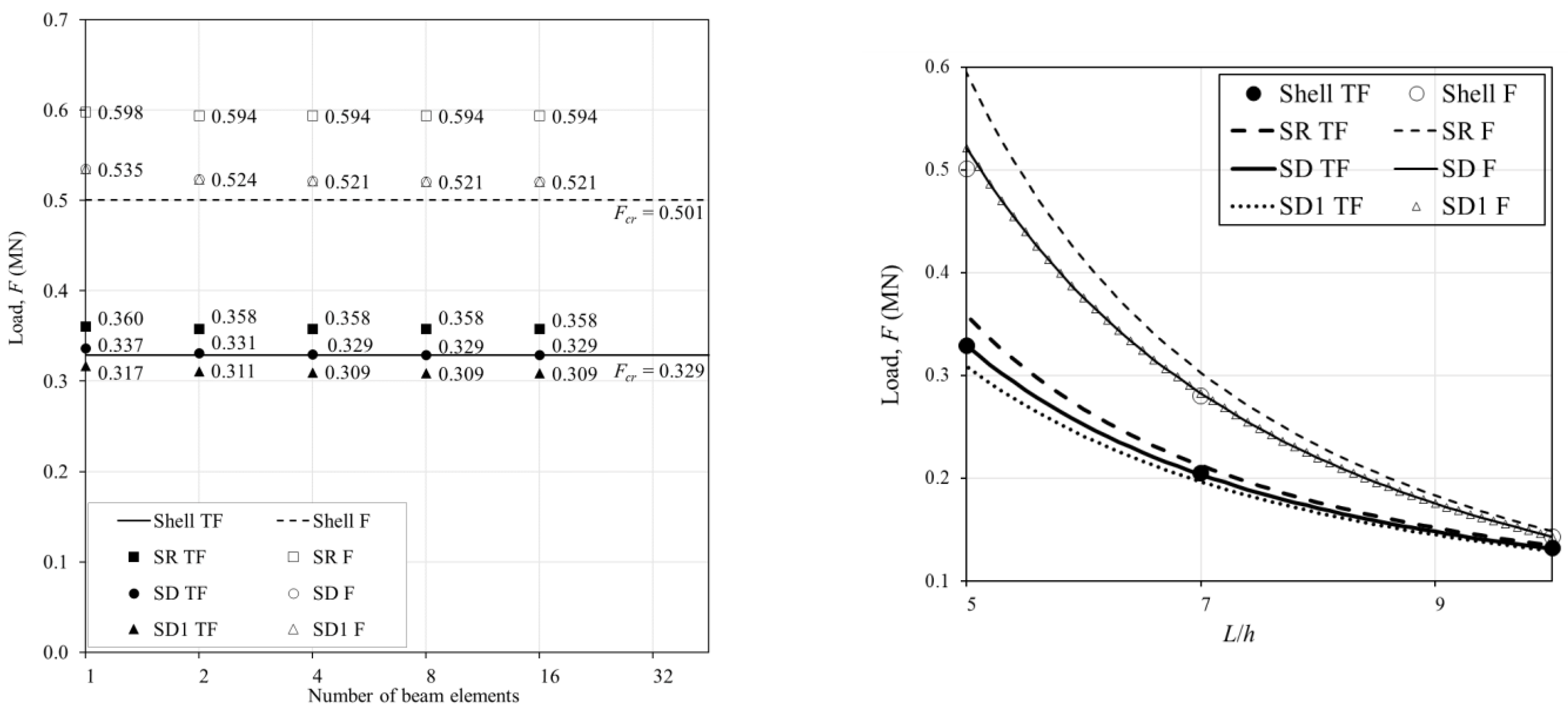
Figure 6.
Cantilever beam: (a) geometry and (b) lateral-torsional buckling mode.
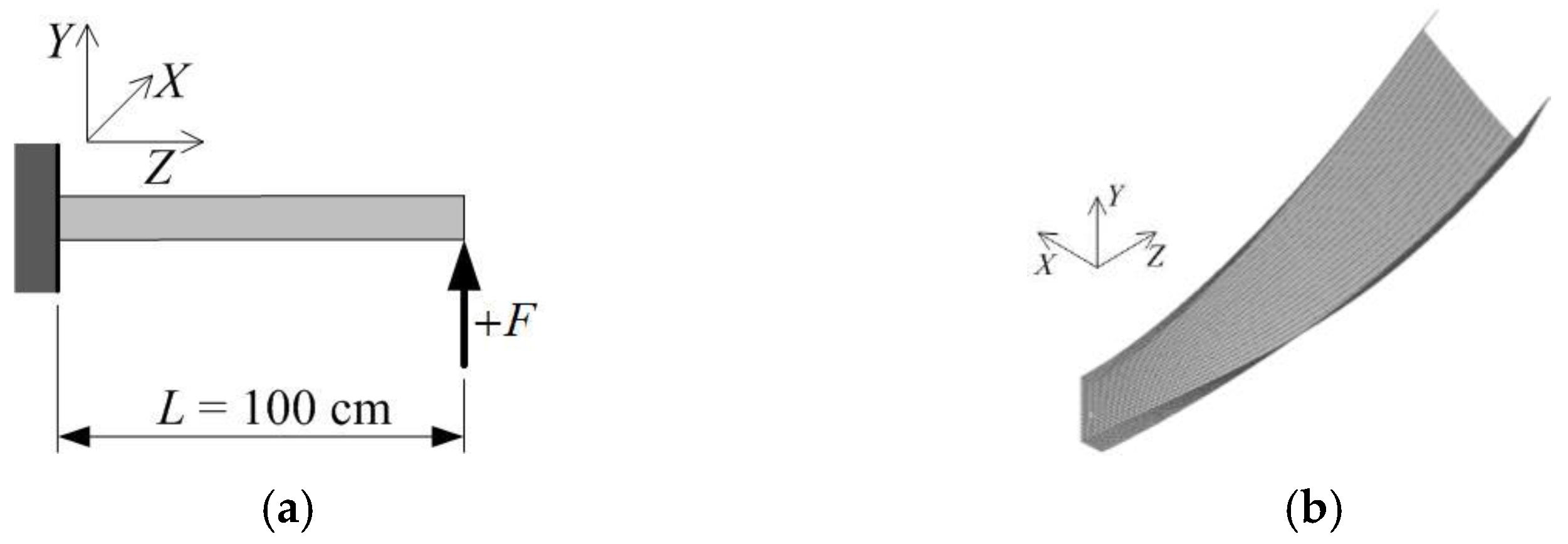
Figure 7.
Buckling load vs. free end displacement in the X-direction: (a) +F and (b) −F.
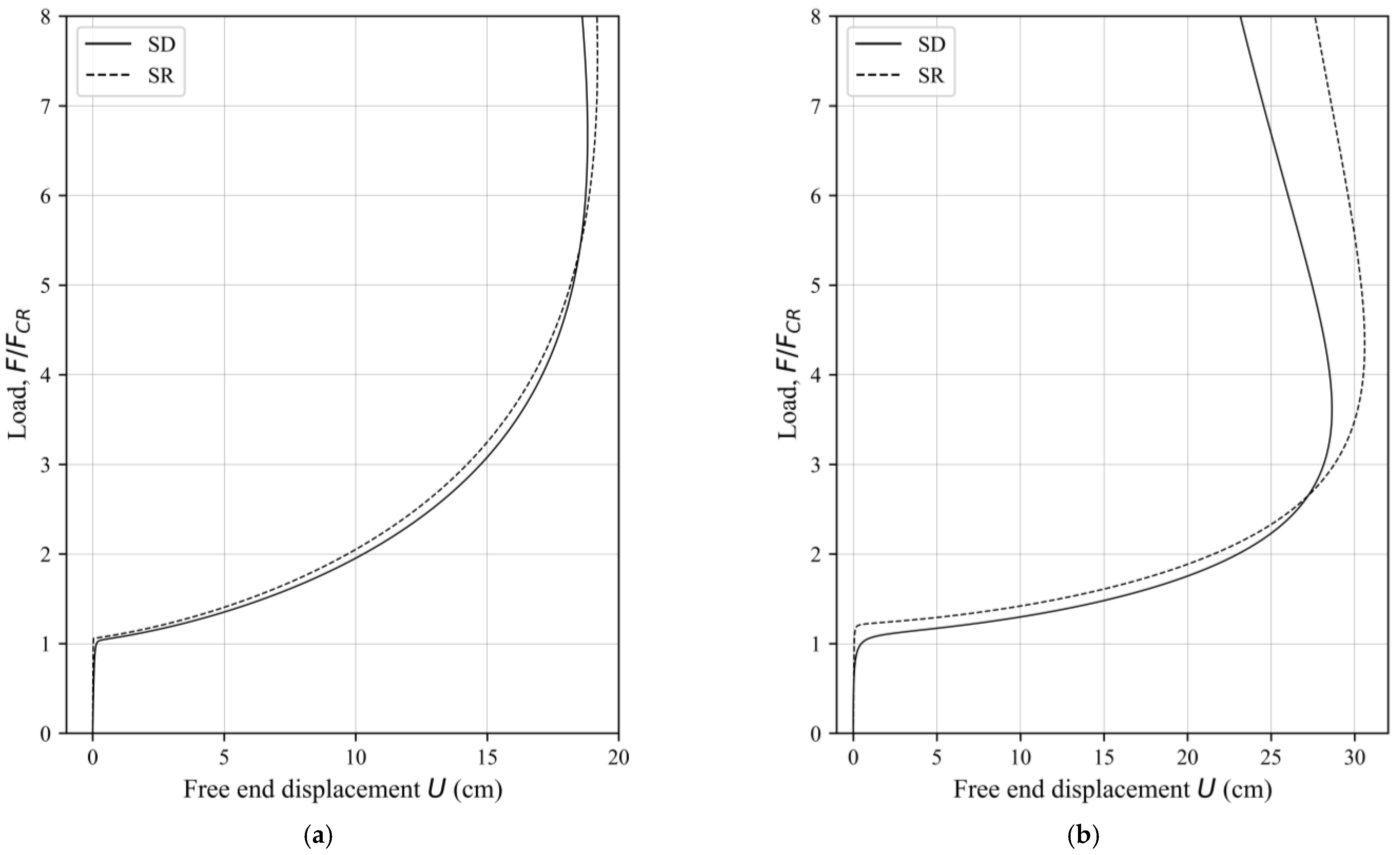
Figure 8.
Buckling load convergence vs. free end displacement in the X-direction: (a) +F and (b) −F.
Figure 8.
Buckling load convergence vs. free end displacement in the X-direction: (a) +F and (b) −F.
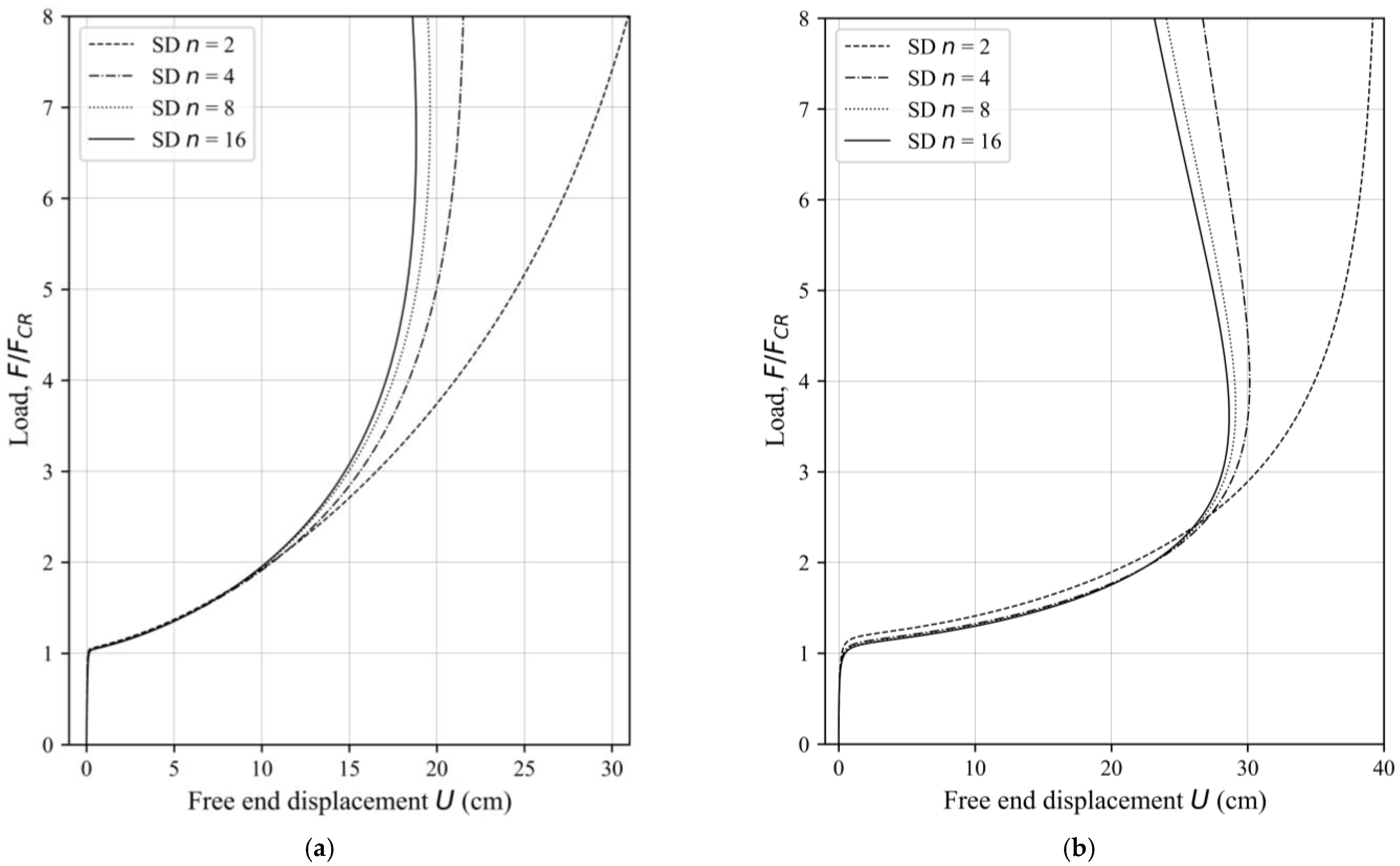
Figure 9.
L-frame: (a) geometry and (b) lateral-torsional buckling mode.
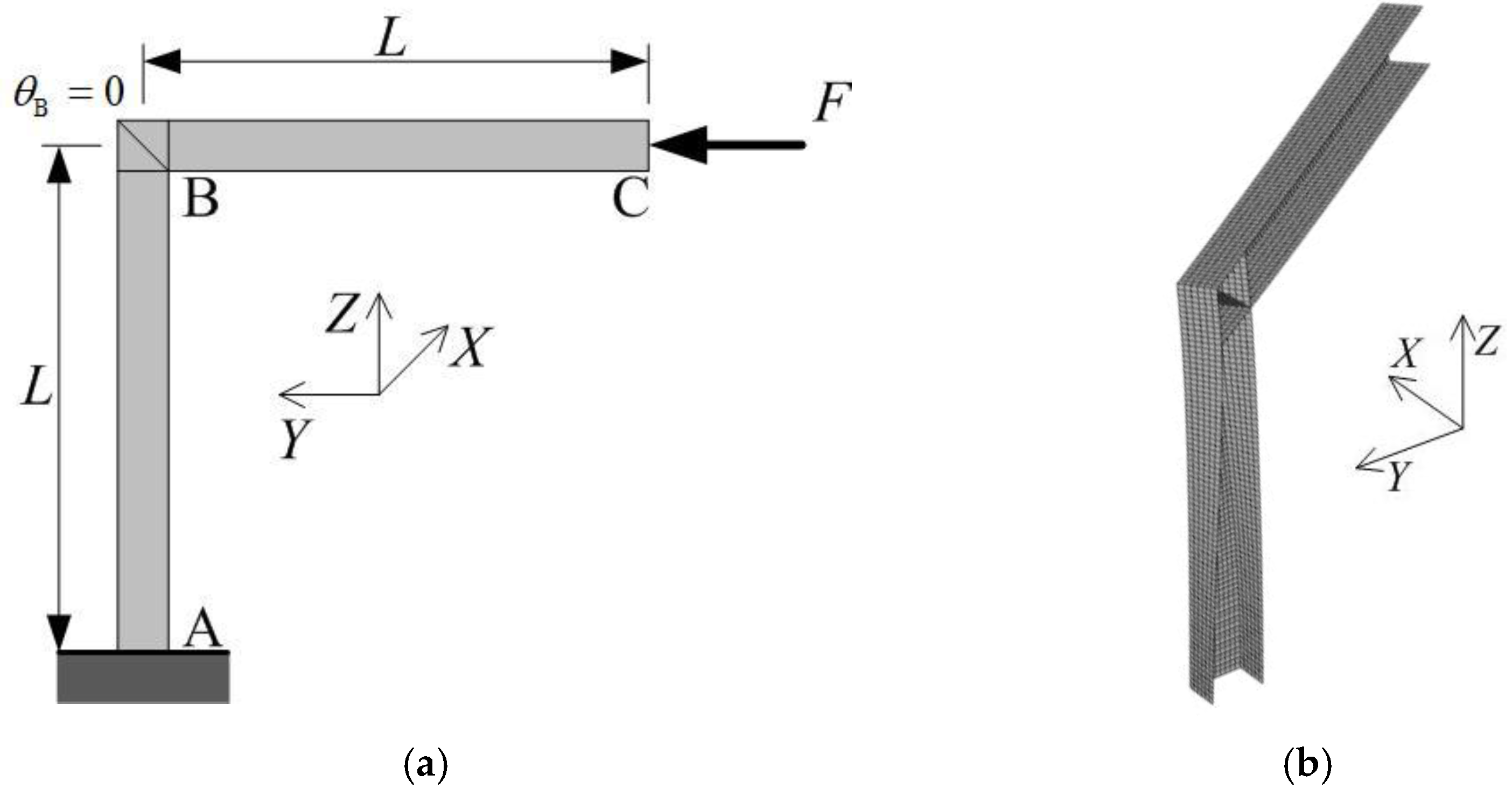
Figure 10.
Buckling load convergence vs. free end displacement in the X-direction: (a) pre-buckling response and (b) post-buckling response.
Figure 10.
Buckling load convergence vs. free end displacement in the X-direction: (a) pre-buckling response and (b) post-buckling response.


Table 1.
Cross-section properties of Examples 1 and 3.
| [0°/90°/0°] | (cm2) | (cm4) | (cm4) | (cm4) | (cm4) | xc (cm) | xg (cm) | xs (cm) |
| 22 | 532.343 | 72.525 | 7.333 | 1718.819 | 3.159 | 4.364 | 5.767 | |
| Kx | Ky | Kω | Kyω | (GPa) | (GPa) | |||
| 2.1504 | 2.3969 | 0.0217 | −0.4999 | 82.932 | 4.14 |
Table 2.
Example 2’s cross-section properties.
| [0°/90°/0°] | (cm2) | (cm4) | (cm4) | (cm4) | (cm4) | xs (cm) | ys (cm) | α (°) |
| 16 | 342.486 | 17.701 | 5.333 | 186.781 | 2.782 | −1.769 | 6.404 | |
| (GPa) | (GPa) | Kx | Ky | Kω | Kxy | Kxω | Kyω | |
| 60.031 | 4.14 | 3.2748 | 1.6373 | 0.0358 | −36.7315 | −1.2571 | −0.7571 |
Publisher’s Note: MDPI stays neutral with regard to jurisdictional claims in published maps and institutional affiliations. |
© 2022 by the authors. Licensee MDPI, Basel, Switzerland. This article is an open access article distributed under the terms and conditions of the Creative Commons Attribution (CC BY) license (https://creativecommons.org/licenses/by/4.0/).
Share and Cite
MDPI and ACS Style
Banić, D.; Turkalj, G.; Kvaternik Simonetti, S.; Lanc, D. Numerical Model for a Geometrically Nonlinear Analysis of Beams with Composite Cross-Sections. J. Compos. Sci. 2022, 6, 377. https://doi.org/10.3390/jcs6120377
AMA Style
Banić D, Turkalj G, Kvaternik Simonetti S, Lanc D. Numerical Model for a Geometrically Nonlinear Analysis of Beams with Composite Cross-Sections. Journal of Composites Science. 2022; 6(12):377. https://doi.org/10.3390/jcs6120377
Chicago/Turabian StyleBanić, Damjan, Goran Turkalj, Sandra Kvaternik Simonetti, and Domagoj Lanc. 2022. "Numerical Model for a Geometrically Nonlinear Analysis of Beams with Composite Cross-Sections" Journal of Composites Science 6, no. 12: 377. https://doi.org/10.3390/jcs6120377