
Modeling of a Process Window for Tailored Reinforcements in Overmolding Processes


1
TUM Department of Mechanical Engineering, Chair of Carbon Composites, Technical University of Munich, 85748 Garching, Germany
2
Polymer Engineering Center (PEC), University of Wisconsin-Madison, 1513 University Ave, Madison, WI 53706, USA
*
Author to whom correspondence should be addressed.
J. Compos. Sci. 2024, 8(2), 65; https://doi.org/10.3390/jcs8020065
Submission received: 10 January 2024
/
Revised: 27 January 2024
/
Accepted: 2 February 2024
/
Published: 8 February 2024
(This article belongs to the Topic Advanced Composites Manufacturing and Plastics Processing)
Abstract
:This study explores cost-effective and customized composite applications by strategically placing carbon fiber-reinforced thermoplastics in multi-material designs. The focus is on developing a model for the simultaneous processing of non-reinforced and reinforced thermoplastic layers, with the aim of identifying essential parameters to minimize insert flow and ensure desired fiber orientation and positional integrity. The analysis involves an analytical solution for two layered power-law fluids in a squeeze flow setup, aiming to model the combined flow behavior of Newtonian and pseudo-plastic fluids, highlighting the impact of the non-Newtonian nature. The behavior reveals a non-linear trend in the radial flow ratio towards the logarithmic consistency index ratio compared to a linear trend for Newtonian fluids. While a plateau regime of consistency index ratios presents challenges in flow reduction for both layers, exceeding this ratio, depending on the height ratio of the layers, enables a viable overmolding process. Therefore, attention is required when selectively placing tailored composites with long-fiber-reinforced thermoplastics or unidirectional reinforcements to avoid operating in the plateau region, which can be managed through appropriate cavity or tool designs.
1. Introduction
Carbon fiber-reinforced composites offer exceptional strength-to-weight ratios, making them highly desirable for lightweight applications in the automotive [1] and aerospace [2] industries. However, the high cost of carbon fibers limits their economic feasibility, particularly in the automotive sector [3]. To overcome this, load-adapted reinforcements are proposed [4], selectively placing composites in load-bearing areas and tailoring fiber direction and length accordingly [5]. Thermoplastics, with their weldability, enable these multi-material designs by combining reinforced and non-reinforced inserts [6]. The advancement of part design optimizations requires varying overmolding layer thicknesses and employing load-adapted reinforcements such as unidirectional and long fiber reinforcements. Modeling the flow of such materials as power-law fluids facilitates understanding of part design’s impact on the transverse flow of composite inserts during processing. The aim is to explore analytically the interplay between part and insert design, processability, and design limitations, offering insights for cost-effective and customized composite applications.
2. A Model for the Transverse Flow of Composite Inserts
The shear flow behavior of filled and unfilled polymers can be modeled as a power-law fluid. A power-law fluid exhibits shear rate-dependent behavior, which characterizes its non-Newtonian nature and plasticity. In the case of a power-law coefficient of 1, the fluid is considered Newtonian, where the shear stress is directly proportional to the shear rate [7]. Conversely, for a pseudo-plastic fluid with a power-law coefficient of zero, the shear stress remains independent of variations in the shear rate [8]. In this context, the shear stress maintains a constant magnitude. Below the critical shear stress, flow ceases, while above it, flow is initiated, marking the transition from a solid-like to a fluid-like state [9]. This critical shear stress is commonly known as the yield stress [10]. Polymers typically exhibit power-law coefficients ranging between 0 and 1, rendering them pseudo-plastic fluids. Notably, an augmentation in filler content amplifies the material’s plastic behavior [11].
When implementing local load-adapted reinforcements, the integration of non-reinforced and reinforced thermoplastic polymer layers occurs via a unified molding process. This process necessitates the establishment of a pressure gradient towards the flow front to facilitate the welding of layers [12,13,14] and mold filling, typically employing the non-reinforced material. These layers are typically arranged in close proximity to each other. It is noteworthy that the pressure gradient can induce transverse flow not only in the non-reinforced layer but also in the reinforced layer [15,16]. Additionally, the presence of the non-reinforced layer generates shear stress on the reinforced layer as an insert [17]. The transverse flow of the reinforced layer, influenced by these processing parameters, might disrupt the desired fiber orientation and positional integrity. Consequently, the derivation of an analytical or semi-analytical model based on constitutive equations for a representative configuration becomes indispensable. Thus far, only analytical models for non-interacting power-law layers [18] have been published. The model in this paper facilitates the identification of relevant process, part design, and material parameters crucial for minimizing insert flow.
3. Constitutive Equations for Squeeze Flow of Two Layered Power-Law Fluids
For the development of an analytical model, the constitutive equations are derived from a squeeze flow experimental arrangement (Figure 1), wherein two circular-shaped specimens with equal radii are positioned between two rigid plates at the center. The variation in inter-plate distance corresponds to the applied closing force. In this context, the closing speed is maintained at a constant value, and the resultant closing force is calculated as the output parameter.
The volume of the specimen remains constant throughout the process. Consequently, the radii of the layers progressively increase as the height decreases. The continuity equation, along with the equations of motion in the radial () and axial () directions, retain their form as in a single-layer squeeze flow setup. Moreover, the boundary conditions at the wall and the plane of symmetry remain unchanged, as schematically shown in Figure 2.
A coordinate system is introduced for each layer, positioned at the flow field’s line of symmetry. Consequently, the actual layer height is substituted with a representative layer height, influenced by the interaction with the second layer. The closing rate at the boundaries of the representative layers undergoes the same transformation. This results in two sets of constitutive equations, which are identical but separately defined for each layer. Their solution is presented in Appendix A, which employs a power-law fluid material model.
The determination of representative heights and their time derivatives for each layer necessitates the inclusion of four additional boundary conditions. These boundary conditions are specified at the interface between the two fluid layers as well as at each position along the radial direction ().
The first boundary condition (Equation (1)) asserts that the pressure remains solely a function of r, and a force balance between layer 1 and layer 2 must be maintained. Consequently, the pressure and pressure gradient in both layers must be equal at every position. The second (Equation (2)) and third (Equation (3)) boundary conditions account for shear force and velocity balance between the first and second layers. These conditions ensure that the shear forces and velocities at the contact of the two layers are consistent with each other. Lastly, the fourth boundary condition (Equation (4)) arises from a mass balance consideration, indicating that the sum of the closing rates of layer 1 and layer 2 at each position along the z-axis must equal the total closing rate.
These boundary conditions yield four equations, and the four unknowns are the representative height and their time derivatives for each layer. Therefore, the term “representative” signifies that these values correspond to a single-layer setup that yields the same pressure gradient, effectively representing the equal flow resistance in radial flow.
4. Solution and Model Validation
The utilization of the boundary conditions yields a solution for each position along the radial direction (), which is discussed first with the resulting dimensionless numbers and their interpretation. The solution is then validated by the investigation of exemplary resulting flow fields and the overall flow rate of each layer for a variation of the consistency index ratios.
4.1. Resulting Solution and Dimensionless Numbers of the Model
The solution for each position along the radial direction () is denoted by Equation (5). The derivation of this equation is given in Appendix B. The factors and (Equations (6) and (7)) in the equation are functions of the ratio between the representative height and the actual height, as well as the ratio of the actual heights of layer 1 and layer 2 at the given radial position. These functions, raised to the power-law index difference between the layers, are interconnected with the overall process setup parameters to the power of the power-law difference, incorporating variables such as the closing speed, radius, and total height. Further parameters are the consistency index ratio and a factor that results from the power-law coefficients as depicted in Equation (6).
Equation (15) demonstrates that the obtained results rely on the radial position, especially when dealing with unequal power-law coefficients. This implies that the height change ratio between layers 1 and 2 varies at each radial position. Consequently, the boundary layer between the two layers deviates from a horizontal line and becomes a function of r over time.
The corresponding rate of change along r of the layer height reduction is not considered within the finite difference analysis in . However, it is considered in a global mass balance calculation to determine the total change in the layer radii. In other words, height reduction is not treated as a function of r within a finite radial element. This simplification is employed in this model to facilitate the utilization of the analytical solution of the squeeze flow equation, leading to a semi-analytical model that allows the identification of dimensionless numbers and their interrelation.
The resulting dimensionless numbers are given by π1, π2, and π3 in Equations (8)–(10).
The first dimensionless number, π1, in Equation (8) is the ratio of the actual layer heights, representing a key design parameter for the part design. The second dimensionless number, π2, in Equation (9) is the ratio of the consistency index ratios, representing a key design parameter for the material selection. The third dimensionless number, π3, in Equation (10) incorporates global parameters, such as the overall dimensions of the setup and the closing speed as a processing parameter.
Furthermore, the resulting equations show that the power-law indices remain independent parameters that cannot be summarized as a dimensionless number, which means that the different combinations of power-law indices will lead to non-similar behaviors in the setup.
4.2. Model Validation—Flow Fields
To validate that the model fulfills the boundary conditions and corresponds to a setup as shown in Figure 2, the flow field in the radial direction at a fixed position in r from a representative setup is investigated. The flow field is a visual representation of the results and allows us to visually evaluate if the results are reasonable and valid combinations of representative single-layer flow fields. For a representative flow field, the consistency indices and the power-law indices for both layers are different. Layer one represents a pseudo-plastic layer with a high consistency index, while layer two represents a Newtonian fluid layer with a low consistency index. The resulting flow field is shown in Figure 3, left.
The line of symmetry for both layers coincides, defining the zero position as per Equation (A12) in Appendix B. At the contact point of the layers, the velocity equals, as indicated by Equation (A3). The velocity gradients differ due to the distinct power-law indices and consistency indices. The pseudo-plastic fluid exhibits a typical shear zone at the wall and a flat “plug-flow” zone in the center, while the Newtonian layer shows the usual parabolic shape. Additionally, the Newtonian layer, with its Blower consistency index, demonstrates a higher overall radial flow rate compared to the pseudo-plastic layer. Despite these differences, the flow fields resemble those of single layers, albeit with a shift in the representative height and flow rate, i.e., closing rate, determined by the pressure gradient balance between the layers as per Equation (A1). When the ratio of consistency indices is decreased (Figure 3, right), the line of symmetry shifts towards the insert layer. In such cases, the Newtonian layer approaches a linear “shear-like” velocity profile. The overall radial flow ratio of the two layers serves as an output for subsequent parameter investigations.
4.3. Effect of Newtonian and Non-Newtonian Layer Combinations
In Figure 4, the ratio of radii is shown for two power-law fluids in a squeeze flow setup, with a constant closing speed applied after a fixed period of time. The square symbols represent the combination of two shear-thinning fluids, approximating pseudo-plastic behavior, while the triangular symbols depict the combination of two Newtonian fluids with a power-law exponent of 1.
In the case of two Newtonian fluids, the radii ratio exhibits a linear decrease with a logarithmic increase in the consistency indices. This reasonably implies that the fluid with a higher consistency index results in a reduced radial extension of the layer compared to the fluid with lower consistency. When both fluids have the same flow resistance, the flow field becomes symmetric, and both layers have identical radial extensions.
In contrast, when dealing with two pseudo-plastic fluids, the radii ratio deviates from a linear relationship and shows a non-linear trend towards the logarithmic consistency index ratio. This results in a plateau region where the dependence between the radii ratio and consistency index ratio strongly reduces for two pseudo-plastic layers compared to two Newtonian layers. Therefore, within a specific range of consistency index ratios, the flow of the pseudo-plastic layer cannot be reduced to the same extent as with two Newtonian fluids, presenting a potential challenge in processing. Only when a sufficient consistency index ratio is reached is the flow of the mixture minimized and becomes comparable to that of two Newtonian layers.
Overall, the diagrams highlight the influence of consistency indices on the radial distribution of power-law fluids in a squeeze flow setup, showcasing the differences between shear-thinning (pseudo-plastic) and Newtonian behavior. Their implications for processing are further analyzed by varying the set of parameters.
5. Implications for the Application of Tailored Reinforcement Inserts
In this chapter, the results are detailed for combinations that are most relevant for typical applications in overmolding and therefore lead to model-based design optimization guidelines for processing and part design.
5.1. Flow Behavior of Pseudo-Plastic Inserts
To investigate the behavior in a representative setup, a combination of a pseudo-plastic layer ( = 0.1, = 0.25) representing a highly filled insert and a thicker Newtonian layer ( = 1, = 1.5) representing an overmolding layer is examined. Figure 5 illustrates the resulting height reduction rate of each layer, plotted against the logarithm of the consistency ratio at the initial state (specifically at r = 0.5R). As the experiment maintains a constant volume, the height reduction rate corresponds to the radius ratio as well. The graph exhibits similar non-linear relations as observed for two pseudo-plastic layers (Figure 4).
Three characteristic regimes can be observed. In Regime 1, the insert has a lower consistency index compared to the overmolding layer, leading to a correspondingly higher height reduction rate. As the consistency index ratio increases, the height reduction rate of the insert decreases until it is surpassed by the height reduction rate of the overmolding layer. This marks the transition to Regime 2, where a plateau region follows. In this region, the height reduction rates of both layers remain within a close range for a wide range of consistency index ratios. Only when the consistency index ratio exceeds a ratio of approximately 3, which marks the beginning of Regime 3, does the height reduction ratio change again. In this zone, the height reduction rate of the overmolding layer increases while the height reduction rate of the insert decreases. At the final consistency index ratios, the height reduction becomes limited to the overmolding layer.
This analysis provides insights into the behavior of the two layers in the representative setup, highlighting the impact of consistency index ratios on the height reduction rates and the dominant flow of the overmolding layer in the later stages of the process.
To investigate the underlying flow principles, additional outputs are presented in Figure 6. The top diagram shows the ratio of the pressure gradient in a combined layer setup as a ratio of a single layer pressure gradient, where the boundary conditions match those of a single layer setup. Thus, this ratio indicates how much of the flow resistance is due to a pressure gradient. The bottom diagram illustrates the corresponding representative heights of the layers, as introduced in the constitutive equations. These representative heights serve as indicators of the flow being driven by drag, as they can only be increased by altering the radial velocity at the contact surface, thereby inducing a shear flow in addition to a pressure-driven squeeze flow.
In Regime 1, the ratios of h1 and the pressure gradient indicate that the flow is similar to the single-layer flow of the insert. The velocity profile remains entirely within the layer height, and the resistance corresponds to the insert’s single-layer flow resistance. The overmolding layer interacts with the shear layer of the insert and is solely dragged, as shown by the lower pressure gradient compared to a single-layer setup.
In Regime 2, the representative height of the overmolding layer decreases and the pressure gradient increases, indicating a shift from drag-driven to pressure-driven squeeze flow. The velocity profile of the insert corresponds to the right side of Figure 3. The overmolding layer is now interacting with the plug flow regime of the insert. The velocity profile shape of the overmolding layer remains relatively similar in this regime, with a change in the representative height. Only the curvatures towards the walls are changing slightly, creating the plateau region in Figure 5. When the velocity of the overmolding layer exceeds that of the inserts, as indicated by the crossing lines in Figure 6, the flow ratio changes more rapidly. This shift is accompanied by a transition from shear-dominated to pressure-dominated squeeze flow. Towards the end of Regime 3, the overmolding layer interacts with the second shear layer of the insert near the wall, which leads to a rapid reduction in the insert flow due to the high slopes in the insert velocity profile.
These findings shed light on the flow principles underlying the interaction between the layers, emphasizing the significance of different zones and their impact on flow resistance. By staying within Zone 3, the processing conditions can be optimized to achieve the desired flow behavior.
5.2. Processing Window Resutling from Part and Material Designs
In composite processing, the design of the insert plays a crucial role in achieving the desired properties. Therefore, a processing window is defined for inserts with varying layer heights. Figure 7 displays the radii ratios after the initial timestep, representing the initial flow ratios of the layers while neglecting edge effects. Three setups are examined: two setups with a total height of 1, for which the insert and overmolding layers are interchanged, and one setup with a total height of 2 and a height ratio of 1.
The graph exhibits the same three zones as observed in the previous results for all setups. This similarity underscores the consistency of the findings based on the chosen dimensionless numbers. The boundaries of the zones are approximated by a linear relationship between the radius ratio and the consistency index ratio. This implies that the transition from one zone to another depends on both the height ratio and the consistency index ratio. Higher height ratios lead to shifts in the transition points towards higher radii ratios and consistency index ratios. Remarkably, the change in total height aligns with the previous results, indicating that the height ratio plays a more significant role in determining the flow ratio than the total height.
By setting the minimization of insert flow as a processing condition, a process window can be defined. It is evident that at a certain consistency index ratio, the flow of the insert ceases. This critical consistency index ratio depends on the height ratio and is higher for thin inserts combined with thick overmolding layers.
These findings emphasize the influence of height ratio and consistency index ratio on flow behavior and provide insights into defining process windows for composite processing. The results highlight the importance of optimizing the design parameters, particularly the height ratio for a given material, to control the flow ratios and achieve the desired flow characteristics in composite materials.
5.3. Model-Based Optimization of Process and Part Design
The model shows two extreme cases. The first is a combination of a thin insert with a high consistency index and a thick overmolding layer. The combination of a sufficient consistency index ratio and height ratio can lead to a complete cessation of flow in the insert. This corresponds to the typical application of an organo sheet based on woven continuous fibers, yielding a high consistency index and a thick overmolding layer, such as for a rib structure.
When the material design is fixed, such as in tailored materials, the height ratio becomes increasingly important, especially for lower consistency index ratios. This means that for well-known examples of inserts like woven or cross-ply configurations, the flow of the insert is not expected to occur as the critical consistency index ratio is not exceeded. However, for selectively placing composites in load-bearing areas and tailoring fiber direction and length accordingly, such as for inserts made of long fiber thermoplastics (LFT) or unidirectional (UD) reinforcements, special attention must be given to the process and part design to prevent insert flow.
In that case, the thickness can be reduced by changing the processing conditions. The thickness can be further reduced by using pre-heated inserts, where only the surface is molten in a pre-heating step. This is depicted in Figure 8. The overmolding layer is not affected by the pre-heating step, but the insert is. Only the molten layer that exceeds the melting temperature is considered part of the squeeze flow setup. Therefore, the layer height that counts for the model is reduced significantly, reducing the expected flow of the insert.
Furthermore, the flow of the insert can be reduced by lowering the pressure gradient in directions in which no flow is required and which are critical for the insert, such as perpendicular to the fiber direction for UD materials. This can be controlled by a suitable cavity or tool design that lowers the gap height in the desired directions. Figure 9 shows the assembly with a tool that partly covers the edges of the insert. The tool blocks the insert from flowing sideways. However, it remains to be demonstrated whether the reduction of the gap height directly leads to a decrease in flow resistance.
5.4. Comparison to Applications and Experimental Results
Several studies have investigated the overmolding process with varying materials and part geometries [19]. The main focus of these studies is the mechanical properties resulting from the buildup of an interface between the overmolding material and the insert. However, the flow of the insert is not being observed or reported for short fiber reinforced, long fiber reinforced, UD, or multi-axial fiber reinforced inserts for different cavity designs. Therefore, these setups should represent processing windows that fall under the above model. Three reasons have been identified for this.
First, the ratio of fiber content between the overmolding material and the insert. The consistency index increases with filler content, as empirically studied for different matrix systems and fillers [20]. This, in principle, increases the consistency index ratio for combinations of unfilled and fiber-filled materials. The same can account for combinations of filled materials with different fiber content, such as LFT overmolding materials combined with UD inserts with a 50% higher filler content [21]. In both cases, the consistency index ratio is moved towards the processing window in Figure 7.
Second, a common shape for the overmolding material is ribs locally attached to a thin laminate, e.g., with height ratios above 10 [6,21,22]. This corresponds to the high height ratios in Figure 7 and the tool design in Figure 9. This shifts the process window to even higher consistency index ratios and enables the combination of a thermoforming process in which the laminate is completely heated through the thickness [22].
Third, for complete overmolding or lower height ratios, the insert is not thermoformed and only heated to the temperature of the mold [23,24,25] or at the surface [26]. This corresponds to a thin molten layer on the insert for welding it with the overmolding layer, as shown schematically in Figure 8.
Further experimental investigation is required to identify the limits of tailoring composite inserts in overmolding parts and material designs. This can be achieved by exploring a broader set of materials and geometry.
6. Conclusions and Outlook
The analytical solution for the squeeze flow of two layers of a power-law fluid shows the interplay between consistency index ratios, height ratios, material design, and part design, which plays a crucial role in ensuring successful processing and achieving the desired properties in the manufacturing and overmolding of thermoplastic composite parts. Composite inserts, modeled as pseudo-plastic materials, show extensive flow compared to the overmolding layer when a critical consistency index ratio is reached. Exceeding this critical ratio is particularly significant for low height ratios between the overmolding layer and the insert. As this combination of parameters is more typical for tailored inserts, the right processing becomes crucial for their implementation. The right processing can include the reduction of flowable layer height by local heating of the insert or an optimized cavity design for a reduced radial pressure gradient.
The model includes some simplifications to reach an analytical solution. Therefore, the results should be seen as a guideline for the most important parameters rather than for predicting the deformation of an insert. To account for the non-isothermal effects of injection overmolding, it is important to consider the effective layer thicknesses in non-steady-state conditions and temperature gradients. These effects arise from using inserts that are pre-heated and molds that are cooler than the solidification temperatures of the materials. In addition, the model can be linked to models for the formation of an interface between the overmolding material and the insert. For more predictive models, the material model can be extended to advanced pseudo-plastic material models and evaluated by finite element models and experiments. Furthermore, this approach can address anisotropic material behavior, particularly for unidirectional inserts, which play a crucial role in load-adapted reinforcements.
Author Contributions
Conceptualization, P.K.W.P., T.A.O. and S.Z.; methodology, P.K.W.P. and T.A.O.; validation, P.K.W.P.; formal analysis, P.K.W.P.; investigation, P.K.W.P.; resources, S.Z. and K.D.; data curation, P.K.W.P.; writing—original draft preparation, P.K.W.P.; writing—review and editing, P.K.W.P., T.A.O., S.Z. and K.D.; visualization, P.K.W.P.; supervision, T.A.O., S.Z. and K.D.; All authors have read and agreed to the published version of the manuscript.
Funding
This research received no external funding.
Data Availability Statement
Data are available on request from the authors.
Conflicts of Interest
The authors declare no conflict of interest.
Appendix A
In this appendix, the solutions for the two sets of constitutive equations are given. The two sets of constitutive equations, which are identical but separately defined for each layer as denoted by the index “i”, are given in Equations (A1)–(A3).
The boundary conditions encompass a no-slip condition (Equation (A5)), denoted by a radial velocity of zero, at the wall. At the centerline, there exists no velocity gradient in the radial direction (Equation (A4)), resulting in a zero z-velocity component at the same location (Equation (A6)). Additionally, the z-velocity assumes a value equal to the closing speed at the wall (Equation (A7)).
Consequently, a solution is obtained for the pressure gradient (Equation (A8)), velocity in the radial direction (Equation (A9)), and velocity in the z-direction (Equation (A10)). The representative heights and closing speeds of each layer serve as unknown variables. To determine the shear stress, a material model based on a power-law fluid is employed. Consequently, the resulting equations (Equations (A8)–(A10)) are analogous to the Stefan equation [27] obtained in a single-layer configuration, but they incorporate a representative layer height and a respective closing rate.
Appendix B
In this appendix, the mathematical proof of Equation (5) is provided.
From Equations (1) and (A8):
From Equations (2) and (A8):
From Equations (4) and (A10):
From Equations (3) and (A9):
From Equations (A15) and (A12):
From Equations (A19) and (A18):
From Equations (A14) and (A16):
From Equations (A11), (A21) and (A16):
From Equations (A13), (A18) and (A23):
From Equations (A24) and (A25):
References
- Ahmad, H.; Markina, A.A.; Porotnikov, M.V.; Ahmad, F. A review of carbon fiber materials in automotive industry. IOP Conf. Ser. Mater. Sci. Eng. 2020, 971, 032011. [Google Scholar] [CrossRef]
- Mehl, K.; Schmeer, S.; Motsch-Eichmann, N.; Bauer, P.; Müller, I.; Hausmann, J. Structural Optimization of Locally Continuous Fiber-Reinforcements for Short Fiber-Reinforced Plastics. J. Compos. Sci. 2021, 5, 118. [Google Scholar] [CrossRef]
- Lowe, J. Woodhead Publishing Series in Textiles, Design and Manufacture of Textile Composites; Long, A.C., Ed.; Woodhead Publishing: Cambridge, UK, 2005; Chapter 11; pp. 405–423. [Google Scholar]
- Jespersen, S.T. Methodology for evaluating new high volume composite manufacturing technologies. Ph.D. Thesis, École Polytechnique Fédérale de Lausanne, Lausanne, Switzerland, 2008. [Google Scholar] [CrossRef]
- Lässig, R.; Eisenhut, M.; Mathias, A.; Schulte, R.T.; Peters, F.; Kühmann, T.; Waldmann, T.; Begemann, W. Serienproduktion von hochfesten Faserverbundbauteilen: Perspektiven für den Deutschen Maschinen- und Anlagenbau; Roland Berger: Munich, Germany, 2012. [Google Scholar]
- Akkerman, R.; Bouwman, M.; Wijskamp, S. Analysis of the Thermoplastic Composite Overmolding Process: Interface Strength. Front. Mater. 2020, 7, 27. [Google Scholar] [CrossRef]
- Bird, R.B.; Armstrong, R.C.; Hassager, O. Dynamics of Polymeric Liquids, 2nd ed.; Wiley: New York, NY, USA, 2010. [Google Scholar]
- Gibson, A.G.; Toll, S. Mechanics of the squeeze flow of planar fibre suspensions. J. Non-Newton. Fluid Mech. 1999, 82, 1–24. [Google Scholar] [CrossRef]
- Nadai, A.; Hodge, P. Theory of Flow and Fracture of Solids, vol. II. J. Appl. Mech. 1963, 30, 640. [Google Scholar] [CrossRef]
- Servais, C.; Luciani, A.; Manson, J.E. Squeeze flow of concentrated long fibre suspensions: Experiments and model. J. Non-Newton. Fluid Mech. 2002, 104, 165–184. [Google Scholar] [CrossRef]
- Coussot, P. Yield stress fluid flows: A review of experimental data. J. Non-Newton. Fluid Mech. 2014, 211, 31–49. [Google Scholar] [CrossRef]
- Yang, F.; Pitchumani, R. Healing of Thermoplastic Polymers at an Interface under Nonisothermal Conditions. Macromolecules 2002, 35, 3213–3224. [Google Scholar] [CrossRef]
- Tierney, J.; Gillespie, J.W. Modeling of In Situ Strength Development for the Thermoplastic Composite Tow Placement Process. J. Compos. Mater. 2006, 40, 1487–1506. [Google Scholar] [CrossRef]
- Lee, W.I.; Springer, G.S. A Model of the Manufacturing Process of Thermoplastic Matrix Composites. J. Compos. Mater. 1987, 21, 1017–1055. [Google Scholar] [CrossRef]
- Barnes, J.A.; Cogswell, F.N. Transverse flow processes in continuous fibre-reinforced thermoplastic composites. Composites 1989, 20, 38–42. [Google Scholar] [CrossRef]
- Jones, R.S.; Wheeler, A.B. Transverse Flow of Fibre-Reinforced Composites. In Third European Rheology Conference and Golden Jubilee Meeting of the British Society of Rheology; Springer: Berlin/Heidelberg, Germany, 1990; pp. 258–260. [Google Scholar]
- Heinle, M.; Drummer, D. Measuring mechanical stresses on inserts during injection molding. Adv. Mech. Eng. 2015, 7, 1–6. [Google Scholar] [CrossRef]
- Lee, S.J.; Peleg, M. Lubricated and nonlubricated squeezing flow of a double layered array of two power-law liquids. Rheol. Acta 1990, 29, 360–365. [Google Scholar] [CrossRef]
- Aliyeva, N.; Sas, H.S.; Okan, B.S. Recent developments on the overmolding process for the fabrication of thermoset and thermoplastic composites by the integration of nano/micron-scale reinforcements. Compos. Part A 2021, 149, 106525. [Google Scholar] [CrossRef]
- Polychronopoulos, N.D.; Vlachopoulos, J. Polymer Processing and Rheology. In Polymers and Polymeric Composites: A Reference Series Book Series; Springer: Berlin/Heidelberg, Germany, 2019. [Google Scholar] [CrossRef]
- Giusti, R.; Lucchetta, G. Analysis of the welding strength in hybrid polypropylene composites as a function of the forming and overmolding parameters. Polym. Eng. Sci. 2017, 58, 592–600. [Google Scholar] [CrossRef]
- Joppich, T.; Menrath, A.; Henning, F. Advanced Molds and Methods for the Fundamental Analysis of Process Induced Interface Bonding Properties of Hybrid, Thermoplastic Composites. Procedia CIRP 2017, 66, 137–142. [Google Scholar] [CrossRef]
- Fu, L.; Ding, Y.; Weng, C.; Zhai, Z.; Jiang, B. Effect of working temperature on the interfacial behavior of overmolded hybrid fiber reinforced polypropylene composites. Polymer Testing 2020, 91, 106870. [Google Scholar] [CrossRef]
- Andrzejewski, J. The Use of Recycled Polymers for the Preparation of Self-Reinforced Composites by the Overmolding Technique: Materials Performance Evaluation. Sustainability 2023, 15, 11318. [Google Scholar] [CrossRef]
- Joo, S.-J.; Yu, M.-H.; Kim, W.S.; Lee, J.-W.; Kim, H.-S. Design and manufacture of automotive composite front bumper assemble component considering interfacial bond characteristics between over-molded chopped glass fiber polypropylene and continuous glass fiber polypropylene composite. Compos. Struct. 2020, 236, 111849. [Google Scholar] [CrossRef]
- Matsumoto, K.; Ishikawa, T.; Tanaka, T. A novel joining method by using carbon nanotube-based thermoplastic film for injection over-molding process. J. Reinf. Plast. Compos. 2019, 38, 616–627. [Google Scholar] [CrossRef]
- Stefan, J. Versuche über die scheinbare Adhäsion. Ann. Physik. 1875, 230, 316–318. [Google Scholar] [CrossRef]
Figure 1.
A schematic representation of a squeeze flow setup consisting of two circular-shaped adjacent fluid layers with different flow properties and heights between two moving rigid plates.
Figure 1.
A schematic representation of a squeeze flow setup consisting of two circular-shaped adjacent fluid layers with different flow properties and heights between two moving rigid plates.
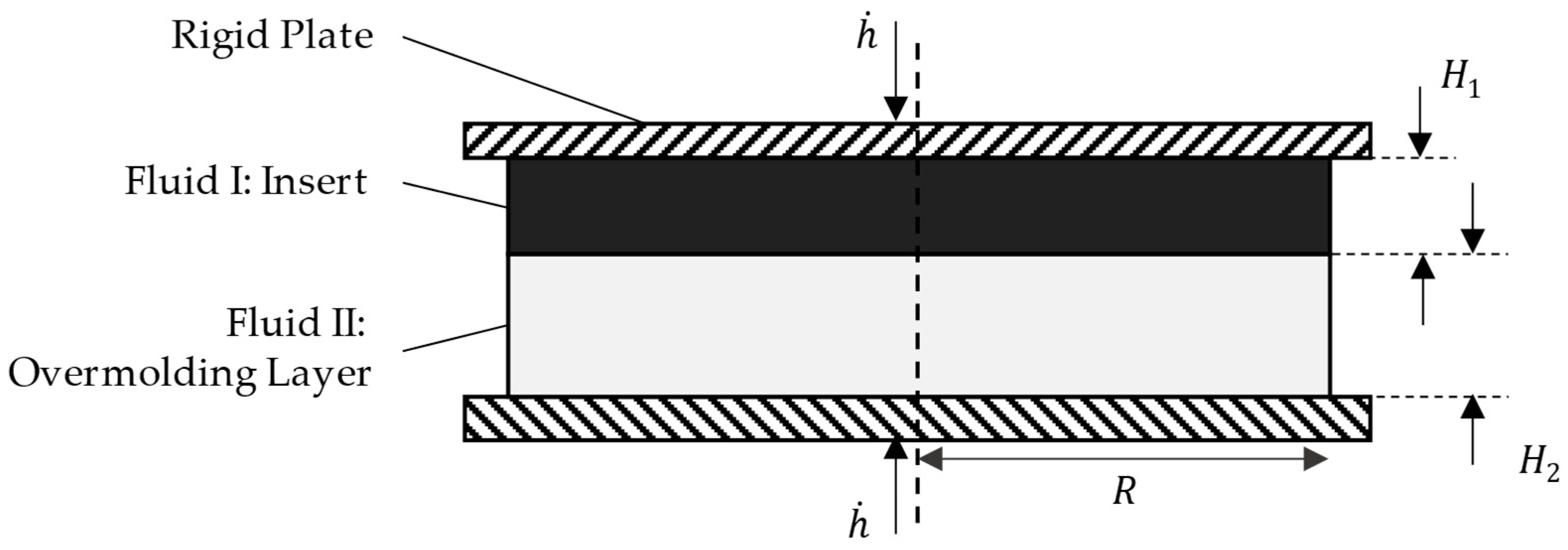
Figure 2.
A schematic representation of a radial velocity profile for two adjacent fluid layers with their representative layer heights and coordinate systems.
Figure 2.
A schematic representation of a radial velocity profile for two adjacent fluid layers with their representative layer heights and coordinate systems.

Figure 3.
Dimensionless radial velocity by the dimensionless position in z for fluid layer 1 and fluid layer 2 with the line of symmetry for both flow fields for two different consistency index ratios.
Figure 3.
Dimensionless radial velocity by the dimensionless position in z for fluid layer 1 and fluid layer 2 with the line of symmetry for both flow fields for two different consistency index ratios.

Figure 4.
Ratio of the radii of two pseudo-plastic and two Newtonian fluid layers as a ratio of their consistency indices.
Figure 4.
Ratio of the radii of two pseudo-plastic and two Newtonian fluid layers as a ratio of their consistency indices.
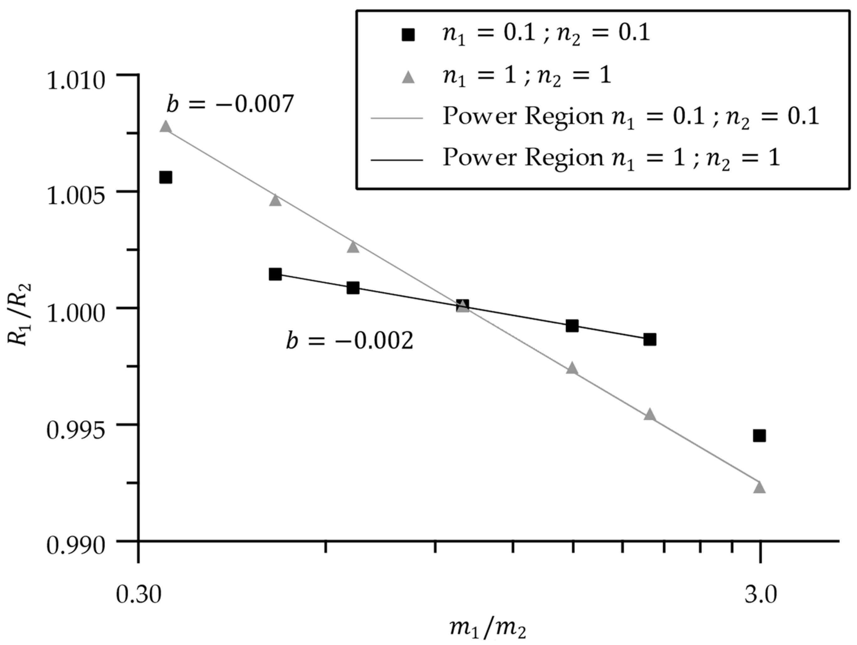
Figure 5.
The height change of the two fluid layers scaled by their height change in a single-layer setup as a ratio of their consistency indices with the indication of three flow zones.
Figure 5.
The height change of the two fluid layers scaled by their height change in a single-layer setup as a ratio of their consistency indices with the indication of three flow zones.

Figure 6.
Pressure gradient of the two fluid layers scaled by their pressure gradient in a single layer setup (top) and their representative height scaled by the total height (bottom) as a ratio of their consistency indices with the indication of three flow zones.
Figure 6.
Pressure gradient of the two fluid layers scaled by their pressure gradient in a single layer setup (top) and their representative height scaled by the total height (bottom) as a ratio of their consistency indices with the indication of three flow zones.
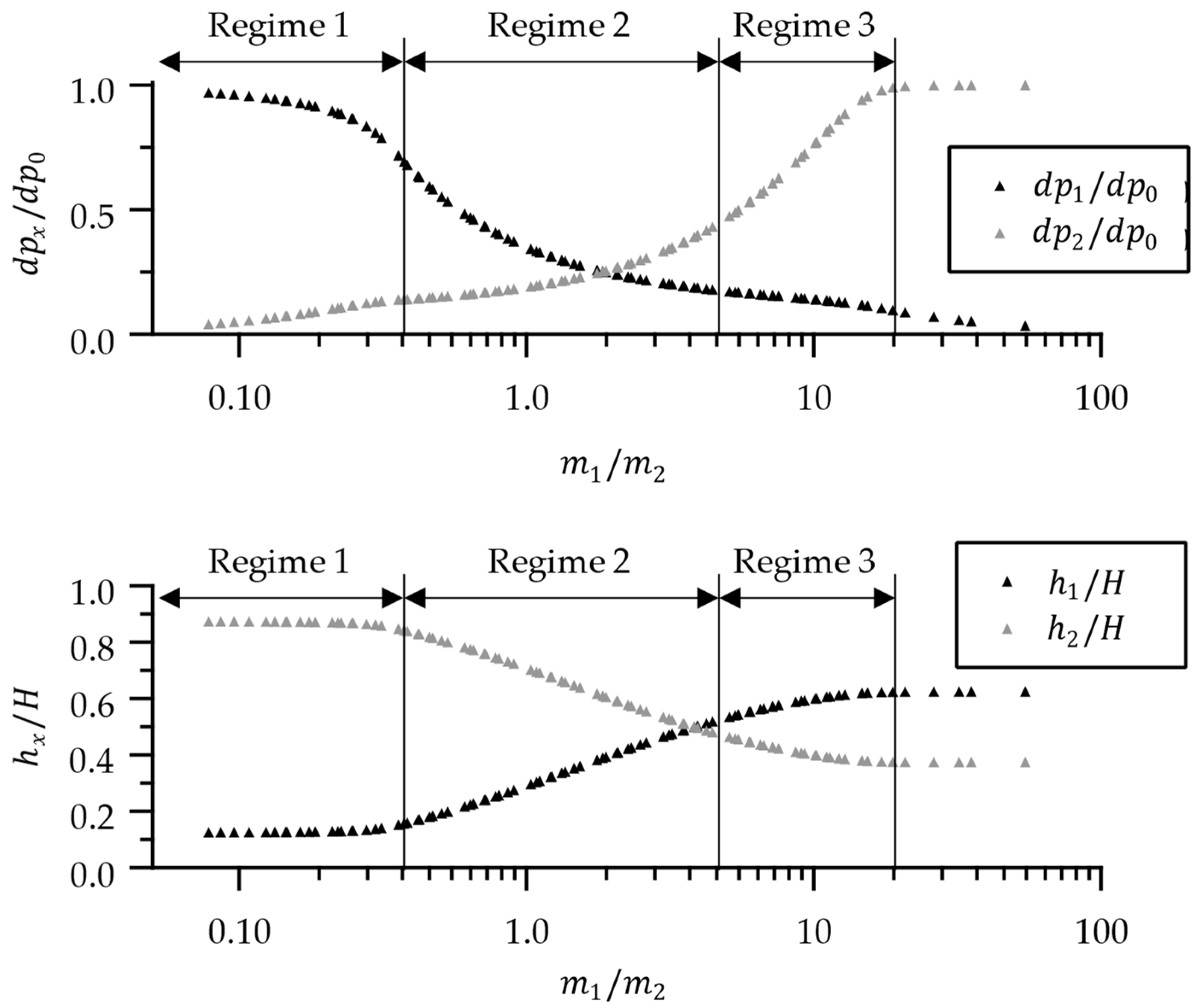
Figure 7.
Ratio of the radii for the combination of a pseudo-plastic and a Newtonian fluid layer at different height ratios as a ratio of their consistency indices with the indication of three flow zones and a process window.
Figure 7.
Ratio of the radii for the combination of a pseudo-plastic and a Newtonian fluid layer at different height ratios as a ratio of their consistency indices with the indication of three flow zones and a process window.
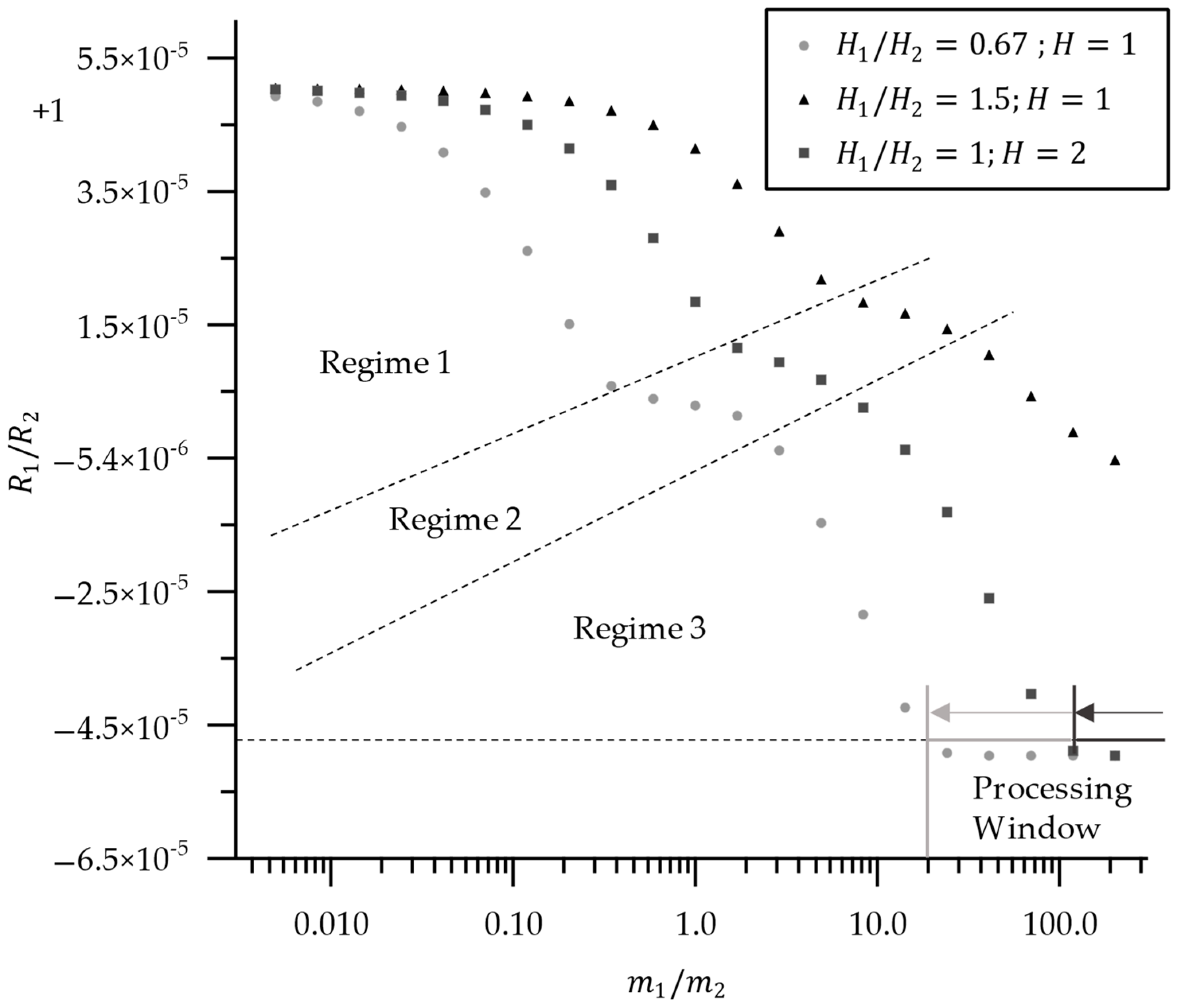
Figure 8.
Schematic representation of an overmolding setup with an overmolding layer and an insert, where the insert consists of a molten and a solidified layer.
Figure 8.
Schematic representation of an overmolding setup with an overmolding layer and an insert, where the insert consists of a molten and a solidified layer.
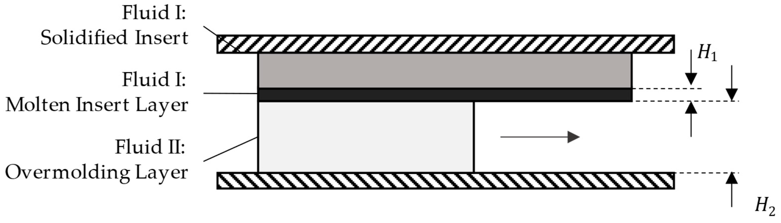
Figure 9.
Schematic representation of an overmolding setup with an overmolding layer and an insert, where part of the insert height is covered by a tool.
Figure 9.
Schematic representation of an overmolding setup with an overmolding layer and an insert, where part of the insert height is covered by a tool.

Disclaimer/Publisher’s Note: The statements, opinions and data contained in all publications are solely those of the individual author(s) and contributor(s) and not of MDPI and/or the editor(s). MDPI and/or the editor(s) disclaim responsibility for any injury to people or property resulting from any ideas, methods, instructions or products referred to in the content. |
© 2024 by the authors. Licensee MDPI, Basel, Switzerland. This article is an open access article distributed under the terms and conditions of the Creative Commons Attribution (CC BY) license (https://creativecommons.org/licenses/by/4.0/).
Share and Cite
MDPI and ACS Style
Picard, P.K.W.; Osswald, T.A.; Zaremba, S.; Drechsler, K. Modeling of a Process Window for Tailored Reinforcements in Overmolding Processes. J. Compos. Sci. 2024, 8, 65. https://doi.org/10.3390/jcs8020065
AMA Style
Picard PKW, Osswald TA, Zaremba S, Drechsler K. Modeling of a Process Window for Tailored Reinforcements in Overmolding Processes. Journal of Composites Science. 2024; 8(2):65. https://doi.org/10.3390/jcs8020065
Chicago/Turabian StylePicard, Philipp K. W., Tim A. Osswald, Swen Zaremba, and Klaus Drechsler. 2024. "Modeling of a Process Window for Tailored Reinforcements in Overmolding Processes" Journal of Composites Science 8, no. 2: 65. https://doi.org/10.3390/jcs8020065