

Ultrasonic Nondestructive Evaluation of Composite Bond Strength: Quantification through Bond Quality Index (BQI)


i-MAPS Laboratory, Department of Mechanical Engineering, University of South Carolina, Columbia, SC 29208, USA
*
Author to whom correspondence should be addressed.
J. Compos. Sci. 2024, 8(3), 107; https://doi.org/10.3390/jcs8030107
Submission received: 9 November 2023
/
Revised: 11 December 2023
/
Accepted: 4 January 2024
/
Published: 18 March 2024
(This article belongs to the Special Issue Feature Papers in Journal of Composites Science in 2023)
Abstract
:This article presents a concept, materials, and methods to devise a Bond Quality Index (BQI) for assessing composite bond quality, approximately correlating to the respective bond strength. Interface bonding is the common mechanism to join two composite structural components. Ensuring the health and quality of the bond line between two load-bearing composite structures is crucial. The article presents the classification and data-driven distinction between two types of bond lines between similar structural components. The interface bonds in composite plates were prepared using polyester peel ply and TX-1040 nylon peel ply. For all the plates, ultrasonic inspection through scanning acoustic microscopy (SAM) (>10 MHz) was performed before and after localized failure of the plate by impinging energy. Energy was impinged 0–10 J/cm2 of in the 16-ply plates, and 0–25 J/cm2 were impinged in 40-ply plates. Followed by bond failure and SAM, a new parameter called the Bond Quality Index (BQI) was formulated using ultrasonic scan data and energy data. The BQI was found to be 0.55 and 0.45, respectively, in plates with polyester peel ply and TX-1040 nylon peel ply bonds. Further, in 40-ply plates with polyester peel ply resulted in a BQI equivalent to 3.49 compared to 0.75 in plates with a TX-1040 nylon peel ply bond. Currently, the BQI is not normalized; however, this study could be used for AI-driven normalized BQIs for all types of bonds in the future.
1. Introduction
Fiber-reinforced polymer composites [1,2] are increasingly used in aerospace applications due to the better stiffness properties and higher strength-to-weight ratio. Adhesive bonds [3] are an integral part of the composite manufacturing process. To build a high strength structure and to ease manufacturability, skins are attached to the reinforcing elements using adhesive bonds [4]. The full advantage of composites could be realized if various parts of a major structure are safely bonded [5,6,7] together. These structures may span from small civil utility structures to large defense structures, e.g., ships and aircraft, made of materials stacked in layers through adhesive bonding [8]. The strength of the structure with adhesive bonds solely depends on the strength, durability, and performance of the bonded parts [9]. Apart from attaining a smoother surface, bonding allows complex shapes and dissimilar materials to be joined together. Adhesive bonding is also a corrosion-resistant, weight-efficient, and cost-effective method compared to other joining methods like bolting, riveting, and welding.
Under different hostile circumstances with a varying temperature and humidity, such adhesive bonds are prone to fatigue defects, yielding failure, resulting in resin crazing, cracks, and disbands [9]. Such occurrences may cause a sudden reduction of interfacial strength, forming cracks, delamination, and damage related to debonding [10,11]. Such defects could result in compromised structural safety and integrity. Other defects may also generate during the assembly, including voids, poor adhesive strength, and poor cohesive joints. Although in earlier days, most detection of the bonding damages was carried out using destructive testing. Different nondestructive evaluation (NDE) techniques were studied to identify flaws such as voids, porosity, and disbonds in different assemblies [12,13]. The flaws are mostly located between the adhesive layer and/or in one of the adherent parts, and may potentially result in adhesive failure.
Nevertheless, the assessment of bond quality followed by the detection of possible disbonding has been a challenging task in the field of NDE to date. Several techniques like X-ray radiography, ultrasonics, and thermography are explored to detect bond-line damage, but may lack the sensitivity or precise capabilities of characterization to detect weak bonds like kissing bonds [10,12,14,15,16]. There is no quantified measure to certify or characterize a bond line, calibrated with respect to their bond strength.
One of the most popular NDE techniques for composite inspection is ultrasonic [9], as it can penetrate internal laminates and is sensitive to small defects. Enhancement of the sensitivity of the ultrasonic NDE method to a specific condition of a bond was previously presented using ultrasonic resonance spectroscopy and some sensitivity to the kissing bonds was demonstrated [17,18,19]. In weakly bonded metals, the additional modelling of the resonating structure, and the introduction of adhesion stiffness parameters, helped to correlate the adhesion strength [20]. Alternatively, hidden small damages were detected by using a Piezo-electric Transducer (PZT) installed on composite coupons and wind turbines. They used ultrasonic guided waves generated by PZTs in pristine and damaged structures [21,22,23]. But such methods have very low sensitivity. Recent research work on using guided waves to detect weak bonds was reported in ref [24]. Moreover, qualitative understanding of bond quality with respect to the bond strength was not performed and may require further research efforts.
The assembly of multiple composite elements into an integrated structure involves bonding processes, comprising of co-bonds or secondary bonds. In co-bonds, a cured composite is assembled with a film adhesive to an uncured laminate layup. Co-bonds and secondary bonds are inspected by different NDE methods used for laminate inspection for voids or disbonds. The choice of an NDE method depends on the configuration of the structure. Light and Kwun [25] show that the presence and absence of defects like disbonds, delaminations, voids, or foreign objects alter the bond quality of a bonded assembly. While there is no consensus on this term, the following factors are known to influence the bond quality: joint type and geometry, adherend material, adhesive type and composition, surface treatment, environmental conditions, curing process, bond line thickness, residual stress, defects (fabrication or in-service), workmanship, and environmental degradation etc. The bond variables [25] are divided into intrinsic and extrinsic properties. When the intrinsic properties affect the cohesive strength (including the degrees of cure, adhesive chemistry, bond line thickness, and presence of voids), the extrinsic properties affect the adhesive strength (including the surface cleanliness, surface contamination, primer type, application, and wetting properties).
It was determined [25] that even if all intrinsic properties were within the tolerance limit, the bond could still fail prematurely due to the extrinsic properties. As a result, a multidisciplinary approach must be taken that combines NDE and fracture mechanics. Despite finding no defects, the inspection of adhesive bonds has an additional requirement, which is the equivalency of the bond strength. Sometimes bond quality and strength or durability are used interchangeably. This is generally not a favorable interchange or term because there are some means of evaluating bond quality, but the only reliable way to measure bond strength is through destructive tests. Fracture mechanics can be used to evaluate joint strength, and the failure of the joint generally occurs from the propagation of cracks, disbands, or delaminations; therefore, bond quality can give an indication of the remaining strength or remaining useful life.
In search of an NDE method to evaluate the strength of adhesive bonds, researchers found it is a difficult task to achieve. Numerous attempts have been made to find a correlation between ultrasonic or other NDE methods with bond strength [19,26,27]. Nondestructive methods for bond-strength evaluation have not been completely successful because the strength parameter measured was in the plastic regime of a material while nondestructive testing is performed in the elastic regime. Sufficiently strong stress waves that can fail weak bonds were found to provide a method to assess the adhesive strength in composite bonds [28,29,30,31,32]. Bond inspection [33] can reduce qualification cost and schedule while eliminating some technical issues associated with traditional mechanical testing.
Thus, in the composite and structure community an index representing the strength of the bond is much desired parameter to assess the bond quality in adhesively bonded composite parts. There is no self-conforming NDE method that exists that can easily quantify the bond strength nondestructively. That being said, it is emphasized here in this study that even if the bond is free from discontinuity or defects (which an NDE method could easily find), the adhesive composite bond between two parts could still be insufficient to hold the design load. In this situation, it is necessary to achieve an NDE-driven process that can quantify the bond quality with the degree of bond strength achieved. A normalized quantity with 1 being best and 0 being the worst quality of the bond should be devised.
The primary objective of this article is to present the results from a series of inspections on the interface bond line in composite plates. To identify the quality of the bond strength, scanning acoustic microscopy (SAM) (>10 MHz) is employed. The interface bonds in composite plates prepared using polyester peel ply and TX-1040 nylon peel ply. Ultrasonic inspections through SAM were performed on all the plates before and after the energy impact on the plates. In this study impact energy was categorized into three types, namely Low energy, Mid energy, and High energy impinges. 0–10 J/cm2 were impinged in the 16-ply plates, whereas 0–25 J/cm2 were impinged in 40-ply plates. The 16-ply plates had a bond line between 10 plies and 6 plies. The 40-ply plates had bond lines between 24 plies and 16 plies. Followed by impact and SAM, a new parameter called the Bond Quality Index (BQI) was formulated using ultrasonic scan data and the energy imparted on the plate. BQIs were found to be 0.55 and 0.45, respectively, in plates with polyester peel ply and TX-1040 nylon peel ply bonds. Further, 40-ply plates with polyester peel ply resulted in a BQI equivalent to 3.49 compared to 0.75 in plates with TX-1040 nylon peel ply bond. This says that consistently, the polyester peel ply bond provides a better bond strength than the TX-1040 nylon peel ply bonds. Such information is invaluable for adhesively bonded composite plate structures. A qualitative understanding of bond strength from a quantitative index is devised in this article. Currently, the BQI is not normalized for different ply numbers, plate thicknesses, material types, and ultrasonic frequencies of inspection. However, this study could be used for an AI-driven normalized BQI for all types of bonds in the future.
2. Materials and Methods
2.1. Sample Preparation and SAM
First, two plates were prepared with 16 plies with dimensions of 220 mm 220 mm shown in Figure 1a,b, called Plate 1 and Plate 2, respectively. Both plates had a bond line between the 10th and 11th ply. The bonds were created using a polyester peel ply and TX-1040 nylon peel ply in Plate 1 and Plate 2, respectively. Next, at the pristine state, the interface bonds were inspected using SAM. The wave velocities in the specimens were calculated from the first arrival of the wave packets arriving from the top surface, the back surface, and the internal bond surface. During the SAM experiments Z-scans were saved with A-scan data at each pixel. Figure 1c shows the schematic of the cross sectional view of the plate and a representative A-scan signal (Plate 2). Ultrasonic signals were collected using 25 MHz acoustic objectives with frequency bandwidth of 35 MHz (between ~15 MHz and ~50 MHz). Figure 1d shows the two Time of Flights (TOFs) of two distinct reflections, one from the bond line (TOF 2) and another from the back side (TOF 1) of the plate observed. TOFs were measured from the reflection received from the top surface of the plate. Further signals were analyzed to find the ratio between the two TOFs.
It is observed that both the plates (Plate 1 and Plate 2) had an inherent curvature, which is obvious due to their shifted neutral axis. The curvature happened due to the nonsymmetric distribution of the piles on either side of the bond line. Figure 2 demonstrates the curvature of the plates through the B-scan obtained from the Plate 1 and Plate 2.
The scans were performed twice on each plate. In one scenario, the ten-ply side is exposed to the ultrasound incidence, and in another scenario, the six-ply side is exposed to the ultrasound incidence. Please note that further analyses were performed after passing the data through the curvature compensation algorithm, such that all pulse echo data are consistent for all the pixels. Figure 3 shows the comparison between the two A-signals collected while inspecting the Plate 2. Figure 3a2 shows the signal when the ten-ply side is exposed and Figure 3b2 shows the signal when the six-ply side is exposed. No apparent damage or defects were detected in Plate 1 and Plate 2. To better categorize the analysis results and identify the defected areas in the specimens if any, the SAM Z-scan signals were saved separately, for four different areas, designated with Zone A, B, C, and D as shown in Figure 2.
2.2. Analysis of SAM Data
In Figure 3a2, approximately 10 peaks were observed before the reflection from the interface bond and in Figure 3a2, approximately 6 peaks were observed before the reflection from the interface bond. This phenomenon occurred in all A-Scan signals stored in Z-scans. To assess the interface bond between the two plates, the traveling time from the top surface to the back surface and the traveling time from the top surface to the interface bond were calculated. The parameter is defined as the ratio of the traveling time from the top surface to the back surface over the traveling time from the top surface to the interface bond (). The ratios (TRs) were calculated over the entire plates and divided into four zones as defined in Figure 2. Next, the means and standard deviations of this ratio were calculated at each zone for both Plate 1 and Plate 2. Figure 4 shows the zonal mean value of the Time-of-Flight ratio and the zonal standard deviation obtained from Plate 1 and Plate 2. Based on Figure 4, it can be realized that the mean value of the Time-of-Flight ratio and the standard deviation in the second plate (Plate 2) is higher compared to Plate 1 for all the zones. It can be seen that the Time-of-Flight ratio is the highest in Zone B and D. A higher Time-of-Flight ratio demonstrates the slowness of the wave, possibly due to the weak bond line between the ten-ply and six-ply laminates. From Figure 4a2, it is not yet possible to hypothesize that the Plate 2 bond might be weaker. The increase in the standard deviation means the Time-of-Flight ratios are more randomly distributed. Although the standard deviation is overall increased in Plate 2, the changes are very small with no acceptable error bound. Thus, the conclusion about the random distribution of the ratio is shrouded.
Figure 4b1,b2 illustrates the mean of Time-of-Flight ratio (TR) and the standard deviation in Plate 1 and Plate 2 calculated using the signals collected from the six-ply side. An increased mean value expresses that the wave signals travel slower in Plate 2, possibly due to a weaker bond, but the percentage of increase in the mean value is lower from the 6-ply side compared to the 10-ply side. The standard deviations were also increased in all the zones except in zone D, but the changes are small and inconclusive about the bond quality.
To investigate further, the normal distribution (not shown) of the Time-of-Flight ratios in all the zones from the two plates were plotted. Time-of-Flight ratio of the back-side reflection time to bond line reflection are plotted for four different regions and was plotted against the density. It was observed that the density of the Time-of-Flight ratio for the second plate is lower in comparison to the first plate. In other words, the interface bond in Plate 2 is possibly weaker compared to Plate 1.
Figure 5a shows certain regions labelled in three different colors to symbolize the degree of energy. Yellow symbolizes the Low energy (0–4 J/cm2), blue circles symbolize Mid energy (4–6 J/cm2), and red circles symbolize High energy (6–10 J/cm2). Indications of damage depending on energy are plotted in Figure 5b. Figure 5c shows the C-scans and B-scans at certain selected locations obtained from the SAM. Interestingly, pulse echo ultrasonic inspection cannot always detect the damage at the Mid energy level. The scans in Figure 5c are 25 mm × 25 mm, using a 50 MHz transducer.
Due to the impact, certain regions experienced bond failure. Detailed thorough inspection across the depth with a higher resolution B-scan confirmed the presence of the broken bond. Figure 6 shows both the plates with broken disbonded regions, depicting shear failure due to the impact. Figure 6a shows the polyester bond (Plate 1) breakage at the location D6, while Figure 6b shows the bond breakage for nylon bond breakage (Plate 2) at the location F2.
2.3. Experimental Summary
At the first stage, two adhesively bonded composites plates were manufactured. Two configurations were used with two different peel plies to vary the bond strength. Mechanical tests were performed using flat wise tension (FWT) to measure interlaminar tensile strength. Scanning Acoustic Microscopy (SAM) scans of the plates were performed before and after impacting the specimens.
The B-scan images collected from both the 6-ply side and the 10-ply side allow us to conclude that the disbond/damage is located at the bond line. The corresponding C-scan image indicates that the damage consists of a cluster of smaller indications. Shear failure is observed in high and mid energy impact on both baseline and nylon plates. When the energy is below 3 J/cm2, there is no clear indication of damage. However, the bond strength needs further evaluation to affirm if any degradation exists.
3. Assessment of Bond Quality Using Bond Quality Index (BQI)
Mechanical flat wise tension test (FWT) is a destructive testing method, whereas SAM is a nondestructive test and provides a better insight of the material health. It can provide the local investigations about the failure mechanisms, like is shown in Figure 6.
A representative of the bond strength can be identified and quantified nondestructively using the proposed method named the Bond Quality Index (BQI). Inspection of the interface bond is performed using SAM. As indicated, SAM analyses were performed using 25 MHz. A schematic of the cross-section of the plates and a sample Time-of-Flight (TOF) signal obtained from the SAM scan is shown in Figure 1. The process designed here is to find the ratio between the two TOFs (TOF 1 and TOF 2, in Figure 1c) obtained from the back-side reflection and the interface reflection, named . Ratio of the amplitudes of the reflected signals from the bond line () to the amplitude of the reflected signal from the backside surface () is defined as .
where, is introduced to track the wave data at each pixel point from the SAM Z-scans. In Figure 7, the landscape of and at different impact test points are shown. From the preliminary indications, it was found that the parameters and could be the potential candidates to formulate the BQI. The following ratios at each pixel point are calculated around the impact site (500 × 500 pixels over 25 mm × 25 mm area). Similarly, the average and from the pristine (P) samples. The average and at each (m-th) damage location are calculated as well where the plates were impacted. These parameters are calculated considering the area of the bond that is damaged at different impact location obtained from the SAM-Scan. It was found that the damaged footprint is a function of the energy of the impact. Hence, the energy of impact will be used as an input parameter to the BQI. The damage footprints are measured and correlated with the energy inputs. An energy function is created with a nonlinear regression method, acting as a function of damage size, i.e., the dimension or diameter of the damage or the size of the damage footprint measured from the SAM scans. The energy function is written as . As the damage diameter increases with increasing energy input, the function will be placed in the denominator to compensate for the effect of energy provided to the bond. is the direct measurement of the existence of the delamination near the bond. measures the overall strength of the materials that are bonded. Hence, to measure the quality of the bond, the Bond Quality Index (BQI) is formulated as:
The index is used to identify the m-th impact location on the plate. The and values in the BQI are the average values collected from and around the damage footprint.
The equation of the BQI is based on the following assumptions and facts. For example, damage size caused by the impact depends on the bond quality. The same energy input (J/cm2) for the two different specimens can cause different damage sizes, depending on their bond quality. A higher-quality bond results in a smaller size of damage. A specimen submerged in water has no obvious effect on the quality of the bonds. Ultrasonic scans are repeatable and consistent from scan to scan. This fact is verified using three different scans at the same spot multiple times. A dimensionless parameter is computed at each impact location. A weaker bond will result in the higher reflected amplitude of ultrasonic signal, and hence, the higher value indicates higher degree of the damaged or weaker bond. A dimensionless parameter is also computed at each impact location. A weaker bond resulted in a slower wave speed from the back surface of the specimen and, hence, the Time-of-Flight ratio decreased with increasing damage or weakness of the bond. That means that the higher value indicates a higher degree of damaged bond. Moreover, the higher energy (in J/cm2) is responsible for causing a higher degree of damage. To compensate for this effect, a new dimensionless parameter is devised, i.e., , where is the average energy used in the impact tests, which is in the Mid energy range (4.5 J/cm2) and is the impact energy used at the m-th spot. With the above parameters, we calculated the Bond Quality Index at each impact location (m-th spot) using the formula below.
Based on the formulation, the BQI will range between 0 and a material-dependent upper bound not fixed yet. To set up an upper limit, many experiments should be conducted, and an AI-driven approach should be adopted. A BQI > 0.7 will signify a higher bond quality than BQI < 0.5, which will signify a poor quality of the bond. The BQI at each test spot both in Plate 1 and Plate 2 are first plotted using a scattered plot. Using the BQI formulation, the Energy (E) vs. Damage size (d) and BQI vs. Energy (E) graph are calculated and plotted in Figure 8, through nonlinear regression. Similar analyses were performed for both Plate 1 and Plate 2. Henceforth, the following equations and are proposed, and the newly proposed Q, S, K, and r parameters obtained for Plate 1 and Plate 2 are presented in Figure 8. To investigate the damage state and the bond quality in both the plates at a constant energy = 6 J/cm2 is selected to estimate the tentative damage size and the respective bond quality in Plate 1 and Plate 2. It was found (Figure 8a) that the same energy input 6 J/cm2 caused different damage sizes in Plate 1 (6 mm) and Plate 2 (7.5 mm). Hence, it can be stated that the quality of bond in Plate 2 is weaker than Plate 1.
Similarly, a BQI at a constant energy input 6 J/cm2 was estimated, and it was found (Figure 8b) that the BQIs of Plate 1 and Plate 2 are 0.55 and 0.45, respectively. Based on the assumptions, it can be stated that Plate 2 had the weaker bond than Plate 1. Hence, Figure 8 indicates the same phenomena. Further, to use the BQI as a function of damage size, the following model equation is proposed:
After an impact test, if the damage size is calculated from the specimen using an NDE method, the earlier equation can be used to estimate the bond quality. However, it is realized that the K, r, Q, and S parameters are the material and structure-dependent parameters of a adhesively bonded composite. It was found from the curve that the BQI decreases with increasing level of impact energy, thus, is assumed to be a decaying phenomenon and a negative exponential function is used. Whereas to create higher size damage, higher energy of impact is required. This pattern appears to follow another exponential function with a positive argument. Thus, the equation for energy is substituted in the equation for to obtain Equation (3).
4. Study and Results with Thickened Plates
4.1. Materials and Method
Two 19-inch by 9-inch plates with IM7/8552 unitape were prepared in a 0/90-degree layup. Both the samples were approximately 7.5 mm thick and consisted of 40 layers. The top sheet had 24 plies and was bonded with the bottom sheet that had 16 plies. This placed the bond line at 60% of the total thickness from the top surface. The samples are named Plate A and Plate C, with the bonds created using TX-1040 peel ply and polyester peel ply, respectively. The samples were scanned to identify pre-existing conditions due to manufacturing defects. Plate B was abandoned due to manufacturing defects and a mal-curing process.
Like the first stage of this study, SAM scans were performed on the specimens. Figure 9a shows the scanning acoustic microscope and Figure 9b shows the schematics of the composite inspection and internal modules in SAM. The scanning procedure was started by exciting an ultrasonic p-wave by means of a 10 MHz transducer supplied by Olympus. The diameter and the focal length of the transducer were 0.5 inches and 1 inch, respectively. The generated signals pass through the water and, after reflection from the top surface, bond line and bottom surface of the specimen are received by the same transducer. Thus, the wave velocities in the specimens were calculated from the first arrival of the wave packets reflected from the top surface, the back surface, and the internal bond surface.
To inspect the TOF ratios in the two plates, Z-scans were performed using 500 × 250 resolutions. The ultrasonic signals were further processed to calculate the Time-of-Flight (TOF) from the bottom surface and the bond line surface of the plate. Figure 9c shows the schematics of the two Times-of-Flight (TOFs) used in the analysis. Figure 10 shows a few sample SAM A-scan signals from the Plates A and C. In Figure 10a–d, the wave peaks due to the top surface reflection, the bond surface reflection, and the back-surface reflections are idenfied. Further signals were processed to find out the ratio between the two TOFs obtained from the back-side reflection and the reflection from the interface bond, like it was conducted in Plate 1 and 2.
4.2. SAM Analysis before Imapct
The SAM scans were performed to validate the presence of pre-existing conditions. Z-scans were performed at each of the eight segments of the plate. The Z-scan registers the ultrasonic wave reflection signals at each of the pixel points on the segments with varying focal depth. To assess the interface bond between the two plates, the travel time of the wave from the top surface to the back surface and the travel time from the top surface to the interface bond were calculated. The ratio of the Time of Flight measured from the top surface to the back surface reflection over the Time of Flight from the top surface to the interface bond () or was calculated at each pixel. As an example, the TOF from the bond surface is shown in Figure 11 for both the plates.
Using the TOF distribution from the bond line surface and the back surface, the distribution of the TOF ratio of the back surface to the bond line surface is determined. The ratio of the TOF distributions is shown in Figure 12. Some of the pre-existing conditions are indicated by the red arrows in Figure 12. Pre-existing conditions are identified to avoid the impact tests at those specific locations.
To compare the bond strengths of the two plates, the probability density distribution of the TOFs for the whole domain of Plate A and C are determined using the TOFs from all the pixel points. Figure 13 compares the normal distributions of TOF ratios or as obtained for Plate A and C. It is evident from Figure 13 that the mean value of the ratio for Plate A is higher than Plate C. This means that the wave travels through the bond and reflected from the back surface (refer to Figure 10) in Plate A propagated more slowly than in Plate C. This may lead to a hypothesis that the bond in Plate A is weaker than that of Plate C. Therefore, a lower amount of energy is required to induce damage in Plate A compared to Plate C.
4.3. SAM Analysis after impact Tests
After impact Z-scans were performed using both the 10 MHz and the 25 MHz transducers. To perform this scan, a rectangular area was selected from each of the plates that contains all the impact points. After configuring the scanning parameters, it was possible to clearly identify the debonding or delamination points in the scanned areas. Figure 14 and Figure 15 contain the SAM scan results after impact tests for Plate A and C, respectively. Figure 14 shows the SAM scan results having debonding marked in red. Similarly, Figure 15 shows the SAM scan result, having debonding points marked in red.
Since the different regions of each plate were tested with a different energy of impact the SAM scanned areas show variable damage intensity in Plate A and C. Based on the energy from 0 J/cm2 to 25 J/cm2, the energy was categorized into five energy levels. Debonding or delamination intensity can also be categorized. Figure 16 shows some of the damaged regions of Plate A as categorized by the energy levels. As mentioned earlier, possibly the bond strength in Plate A was weaker than that of Plate C and, hence, within a 15 J/cm2 delamination or debonding are clearly visible. On the other hand, Figure 17 shows some of the damaged regions of Plate C as categorized by the energy level. It can be noted that none of the regions were affected by an energy level less than 10 J/cm2. Since the bond strength in Plate C is higher than that of Plate A, a higher energy was required to induce debonding or delamination in Plate C, which was pre-hypothesized using the SAM data before the impacts.
4.4. BQI Calculation
SAM scans were completed on the pristine samples before the impacts and the average and were determined. The impact energies were categorized in three levels, Low, Medium, and High. After the impacts, the average and at each (m-th) damage location were calculated. Based on the behavioral understanding of the data, the Bond Quality Index (BQI) is defined. In defining the BQI, the following steps were followed.
Step 1: calculate the average and from the pristine (P) samples before the imapct.
Step 2: calculate the average and at each (m-th) damage location where the plated were impacted.
Step 3: a dimensionless parameter is computed at each impact site. A weaker bond results higher reflected amplitude of ultrasonic signal, and hence, a higher value indicates a higher degree of defected or weaker bond.
Step 4: a dimensionless parameter / is computed at each impact site. A weaker bond resulted in a slower wave speed of the signal reflected from the back surface of the specimen and hence, the Time-of-Flight ratio decreased with the increasing damage of the bond. This means that the higher / value indicates a higher degree of defected or weaker bond.
Step 5: a dimensionless parameter is devised, where is the average energy used in the impact tests which is in the Mid energy range (4.5 J/cm2) and is the impact energy used at the m-th spot.
Step 6: the bond parameter at each impact site (m-th spot) was calculated using the formula in Equation (2).
Next, using the steps above, the Energy vs. Damage diameter and BQI vs. impact energy graphs were created as shown in Figure 18 and Figure 19, respectively. From Figure 18, it is evident that Plate C requires a higher impact energy compared to Plate A to induce a similar damage in the bond surface. For example, to induce a damage of a 6 mm diameter, Plate A requires 11 J/cm2 energy whereas Plate C requires 22 J/cm2. Hence, it can be concluded that bond strength in Plate A is weaker than that of Plate C. However, this conclusion is biased by the damage diameter and, thus, the BQI estimation is necessary, which is independent of the damage sizes.
The proposed bond quality index parameter BQI is independent of the damage diameter and establishes a relationship with the ultrasonic test parameters and the impact energies. From Figure 19, it can be seen that with an increasing impact energy, BQI decreases, indicating a higher debonding or delamination condition, which is also evident in the first stage of the results presented in Figure 8.
5. Conclusions
Among composite and structure community, requirement of a Bond Quality Index (BQI) was repeatedly identified for assessing the bond quality in adhesively bonded composite parts. There is no self-conforming NDE method that exists that can easily quantify the bond strength nondestructively. Many different methods including guided-wave ultrasonic techniques have been used to assess the bond quality but fail to assess the state of the bond in comparison to a desired bond strength. That being said, it is emphasized here in this study that even if the bond is free from discontinuity or defects (which an NDE method could easily find), the adhesive composite bond between two parts could still be insufficient to hold the design load. In this situation, it is necessary to achieve an NDE-driven process that can quantify the bond quality with the degree of bond strength achieved.
A normalized quantity, with 1 being best and 0 being worst quality of the bond, should be devised. This article presents a step forward in achieving this goal, although many follow-up research activities must be conducted by the community using Machine Learning and AI. The algorithm devised to determine the Bond Quality Index or BQI in this article is to classify a strong bond from a weak one. In developing the BQI, ultrasonic test parameters derived from acoustic microscopy were utilized. Wave reflection data from the back surface and the bond surface of the plate were determined.
The capability of a BQI could be expanded to make it dependent on only a impact test data and further rely on ultrasonic SAM data to quantify the BQI. Extensive and rigorous impact testing would not be necessary in the future to access the bond strength. Statistical analysis of the SAM data can feed the analysis to provide reliable information on the strength of the bonds. It has been evident that the SAM data can predict the strength of the bonds. The results obtained in the article suggest that the accuracy of SAM data is well suited to formulate the bond quality index parameter.
Author Contributions
Conceptualization, S.B.; methodology, S.B.; software, S.B.; formal analysis, S.B. and V.T.; investigation, V.T.; resources, S.B.; data curation, V.T. and M.M.I.; writing—original draft preparation, S.B. and V.T.; writing—review and editing, M.M.I.; project administration, S.B.; funding acquisition, S.B. All authors have read and agreed to the published version of the manuscript.
Funding
NASA Grant no. NNL15AA16C, 80LARC17004 and NNL09AA00A and for the financial support for this two-phase study.
Data Availability Statement
All scans and ultrasonic SAM raw data and the analysis data will be available from the i-MAPS website, “https://research.cec.sc.edu/banerjee (accessed on 4 January 2024)” after making reasonable request.
Acknowledgments
Authors acknowledge NASA Grant no. NNL15AA16C, 80LARC17004 and NNL09AA00A and for the financial support for this two-phase study. Authors would like to acknowledge technical insight provided by Christopher Deemer with Northrop Grumman, Utah.
Conflicts of Interest
The authors declare no conflict of interest.
Abbreviation Used in Text
| BQI | Bond Quality Index |
| NDE | Nondestructive Evaluation |
| NDI | Nondestructive Inspection |
| SAM | Scanning Acoustic Microscopy |
| PZT | Piezoelectric Transducer |
| TOF | Time of Flight |
| HHUT | Hand-held Ultrasonic Testing |
| FWT | Flat Wise Tension Test |
| TR | TOF Ratio |
References
- Talreja, R.; Varna, J. Modeling Damage, Fatigue and Failure of Composite Materials; Elsevier: Amsterdam, The Netherlands, 2015. [Google Scholar]
- Reifsnider, K.L.; Case, S. Damage Tolerance and Durability of Material Systems; Wiley-VCH: Hoboken, NJ, USA, 2002; p. 435. ISBN 0-471-15299-4. [Google Scholar]
- Davies, P. 16—Adhesive bonding of composites. In Adhesive Bonding, 2nd ed.; Woodhead Publishing Series in Welding and Other Joining Technologies; Woodhead Publishing: Sawston, UK, 2021. [Google Scholar]
- Pantelakis, S.; Tserpes, K.I. Adhesive bonding of composite aircraft structures: Challenges and recent developments. Sci. China Phys. Mech. Astron. 2013, 57, 2–11. [Google Scholar] [CrossRef]
- Adams, R.D.; Comyn, J.; Wake, W.C. Structural Adhesive Joints in Engineering; Springer Science & Business Media: Berlin/Heidelberg, Germany, 1997. [Google Scholar]
- Banea, M.D.; da Silva, L.F. Adhesively bonded joints in composite materials: An overview. Proc. Inst. Mech. Eng. Part L J. Mater. Des. Appl. 2009, 223, 1–18. [Google Scholar] [CrossRef]
- Russell, J.D. Composites affordability initiative: Successes, failures—Where do we go from here? SAMPE J. 2007, 43, 26–36. [Google Scholar]
- Ji, G.; Ouyang, Z.; Li, G. Local interface shear fracture of bonded steel joints with various bondline thicknesses. Exp. Mech. 2012, 52, 481–491. [Google Scholar] [CrossRef]
- Crane, R.L.; Hart-Smith, J.; Newman, J. 8—Nondestructive inspection of adhesive bonded joints. In Adhesive Bonding, 2nd ed.; Woodhead Publishing Series in Welding and Other Joining Technologies; Woodhead Publishing: Sawston, UK, 2021; pp. 215–256. [Google Scholar]
- Crane, R.L.; Dillingham, G. Composite bond inspection. J. Mater. Sci. 2008, 43, 6682–6694. [Google Scholar] [CrossRef]
- Hart-Smith, L.J. An engineer asks: Is it really more important that paint stays stuck on the outside of an aircraft than that glue stays stuck on the inside? J. Adhes. 2006, 82, 181–214. [Google Scholar] [CrossRef]
- Adams, R.D.; Drinkwater, B.W. Non–destructive testing of adhesively–bonded joints. Int. J. Mater. Prod. Technol. 1999, 14, 385–398. [Google Scholar] [CrossRef]
- Munns, I.; Georgiou, G.J. Non-destructive testing methods for adhesively bonded joint inspection: A review. Insight 1995, 37, 941–952. [Google Scholar]
- Cawley, P.; Adams, R.D. Defect types and non-destructive testing techniques for composites and bonded joints. Mater. Sci. Technol. 1989, 5, 413–425. [Google Scholar] [CrossRef]
- Maldague, X. Theory and Practice of Infrared Technology for Nondestructive Testing; Wiley: Hoboken, NJ, USA, 2001. [Google Scholar]
- Ehrhart, B.; Ecault, R.; Touchard, F.; Boustie, M.; Berthe, L.; Bockenheimer, C.; Valeske, B. Development of a laser shock adhesion test for the assessment of weak adhesive bonded CFRP structures. Int. J. Adhes. Adhes. 2014, 52, 57–65. [Google Scholar] [CrossRef]
- Maeva, E.; Severina, I.; Bondarenko, S.; Chapman, G.; O’Neill, B.; Severin, F.; Maev, R.G. Acoustical methods for the investigation of adhesively bonded structures: A review. Can. J. Phys. 2004, 82, 981–1025. [Google Scholar] [CrossRef]
- Marty, P.N.; Desai, N.; Andersson, J. NDT of kissing bond in aeronautical structures. In Proceedings of the 16th World Conference on NDT, Montreal, QC, Canada, 30 August–3 September 2004. [Google Scholar]
- Drewry, M.A.; Smith, R.A.; Phang, A.P.; Yan, D.; Wilcox, P.; Roach, D.P. Ultrasonic techniques for detection of weak adhesion. Mater. Eval. 2009, 67, 1048–1058. [Google Scholar]
- Lévesque, D.; Legros, A.; Michel, A.; Piché, L. High resolution ultrasonic interferometry for quantitative nondestructive characterization of interfacial adhesion in multilayer (metal/polymer/metal) composites. J. Adhes. Sci. Technol. 1993, 7, 719–741. [Google Scholar] [CrossRef]
- Lissenden, C.J.; Rose, J.L. Structural Health Monitoring of Composite Laminates through Ultrasonic Guided Wave Beam Forming; NATO Applied Vehicle Technology: Båstad, Sweden, 2008; pp. 1–14. [Google Scholar]
- Cawley, P. The impedance method of non-destructive inspection. NDT Int. 1984, 17, 59–65. [Google Scholar] [CrossRef]
- Giurgiutiu, V.; Redmond, J.M.; Roach, D.P.; Rackow, K. Active sensors for health monitoring of aging aerospace structures. In Smart Structures and Materials 2000: Smart Structures and Integrated Systems; International Society for Optics and Photonics: Bellingham, WA, USA, 2000. [Google Scholar]
- Roth, W.W. Nondestructive Evaluation and Health Monitoring of Adhesively Bonded Composite Structures. Doctoral Dissertation, University of South Carolina, Columbia, SC, USA, 2017. [Google Scholar]
- Light, G.; Kwun, H. Nondestructive Evaluation of Adhesive Bond Quality: State of the Art Review; Nondestructive Testing Information Analysis Center: San Antonio, TX, USA, 1989. [Google Scholar]
- Cawley, P. Low frequency NDT techniques for the detection of disbonds and delaminations. Br. J. Non-Destr. Test. 1990, 32, 454–461. [Google Scholar] [CrossRef]
- Heslehurst, R.B. Optical NDT of adhesively bonded joints. Mater. Eval. 2009, 67, 837–842. [Google Scholar]
- Bossi, R.; Housen, K.; Walters, C.T.; Sokol, D. Laser bond testing. Mater. Eval. 2009, 67, 819–827. [Google Scholar]
- Perton, M.; Blouin, A.; Monchalin, J.P. Laser shock waves for adhesive bond testing. J. Phys. D Appl. Phys. 2010, 44, 034012. [Google Scholar] [CrossRef]
- Bossi, R. NDE for Adhesive Bond Strength. In Spring Conference 2011; Springer: New York, NY, USA, 2011. [Google Scholar]
- Bossi, R.; Lahrman, D.; Sokol, D.; Walters, C. Laser Bond Inspection for adhesive bond strength. In Proceedings of the International SAMPE Technical Conference, Paris, France, 28–29 March 2011. [Google Scholar]
- Bossi, R.; Giurgiutiu, V. Nondestructive testing of damage in aerospace composites. In Polymer Composites in the Aerospace Industry; Elsevier: Amsterdam, The Netherlands, 2015; pp. 413–448. [Google Scholar]
- Gardiner, G.J. Certification of bonded composite primary structures. In High-Performance Composites; Composite World: Cincinnati, OH, USA, 2014; pp. 50–57. [Google Scholar]
Figure 1.
(a,b) Two received plates, (a) the first plate (b) the second plate, (c) schematic of the plate with 10ply and 6-ply, (d) a sample A-scan signal from Plate 2.
Figure 1.
(a,b) Two received plates, (a) the first plate (b) the second plate, (c) schematic of the plate with 10ply and 6-ply, (d) a sample A-scan signal from Plate 2.

Figure 2.
(a1) Plate 1. (a2) A sample B-scan from the 10-layer side of Plate 1. (b1) Plate 2. (b2) A sample B-scan from the 6-layer side of Plate 2. Due to inherent nonsymmetric distribution of plies on either side of the bond causes an inherent curvature in the plate, the 10-ply side is under tension and 6-ply side is under compression; (c1–c4) shows the probability density of the ratio of TOF1 to TOF2 at the four identified zones in (a1,b1), the red density is for Plate 1 and the blue density is for Plate 2. The red and blue dotted lines show the mean values of the distributions.
Figure 3.
A-scan signals collected from a specific location on Plate 2 (a1,a2) 10 plies on top, (b1,b2) 6 plies on the top.
Figure 3.
A-scan signals collected from a specific location on Plate 2 (a1,a2) 10 plies on top, (b1,b2) 6 plies on the top.
Figure 4.
The Time-of-Flight ratio (TR) in all the four zones while 10-ply side is exposed to ultrasound. (a1) Mean value of Time-of-Flight ratio, (a2) standard deviation of Time-of-Flight ratio, and when the 6-ply side is exposed to ultrasound, (b1) mean value of Time-of-Flight ratio, (b2) standard deviation of Time-of-Flight ratio.
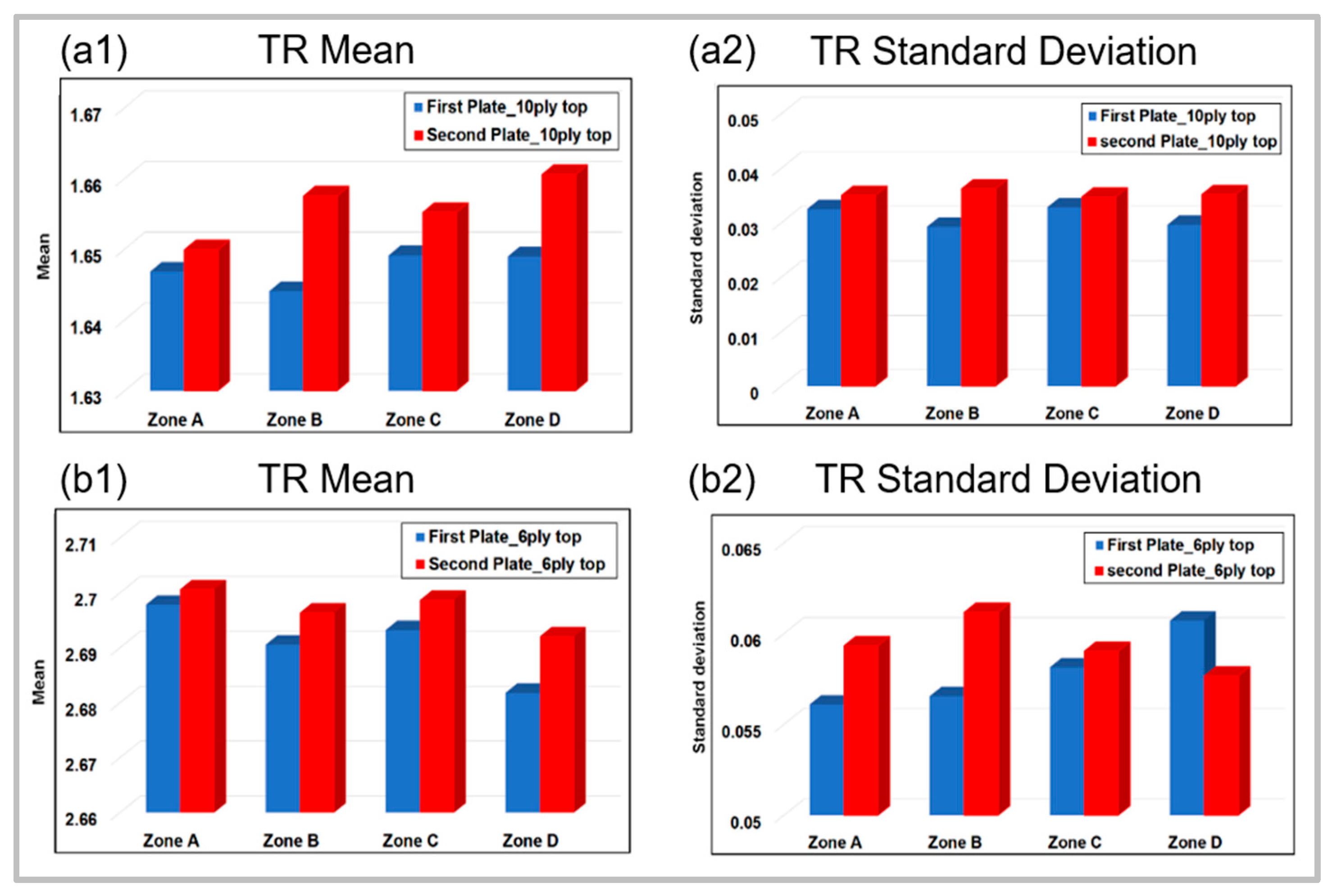
Figure 5.
(a) Points selected from the SAM scans after impact, (b) shows the pulse echo ultrasonic testing results with 0 or 1 indication of damage with respect to the impact energy. (c) shows the C-scan and B-scan images at a few selected points with Low, Medium, and High energy.
Figure 5.
(a) Points selected from the SAM scans after impact, (b) shows the pulse echo ultrasonic testing results with 0 or 1 indication of damage with respect to the impact energy. (c) shows the C-scan and B-scan images at a few selected points with Low, Medium, and High energy.

Figure 6.
Typical scenarios of broken bonds from impact, through NDE inspection across depth, (a) D6 of the plate with polyester peel ply, (a1) shows the zoomed view of the location of the failure of the bond. (b) F2 of the plate with nylon peel ply, (b1) shows the shear failure pattern of the bond in further zoomed in view; (c) demonstrates the results obtained from a few sample FWT tests on both types of bonds. FWT is a destructive test and shows that the nylon peel ply bonds are weaker as an authoritative source of truth; (d) demonstrates the probability of debonding of the bond. It is indicative that the nylon peel ply bonds were weaker, as they take less energy to cause a higher probability of debonding.

Figure 7.
Wd and Rd maps at different impact points after impact tests.
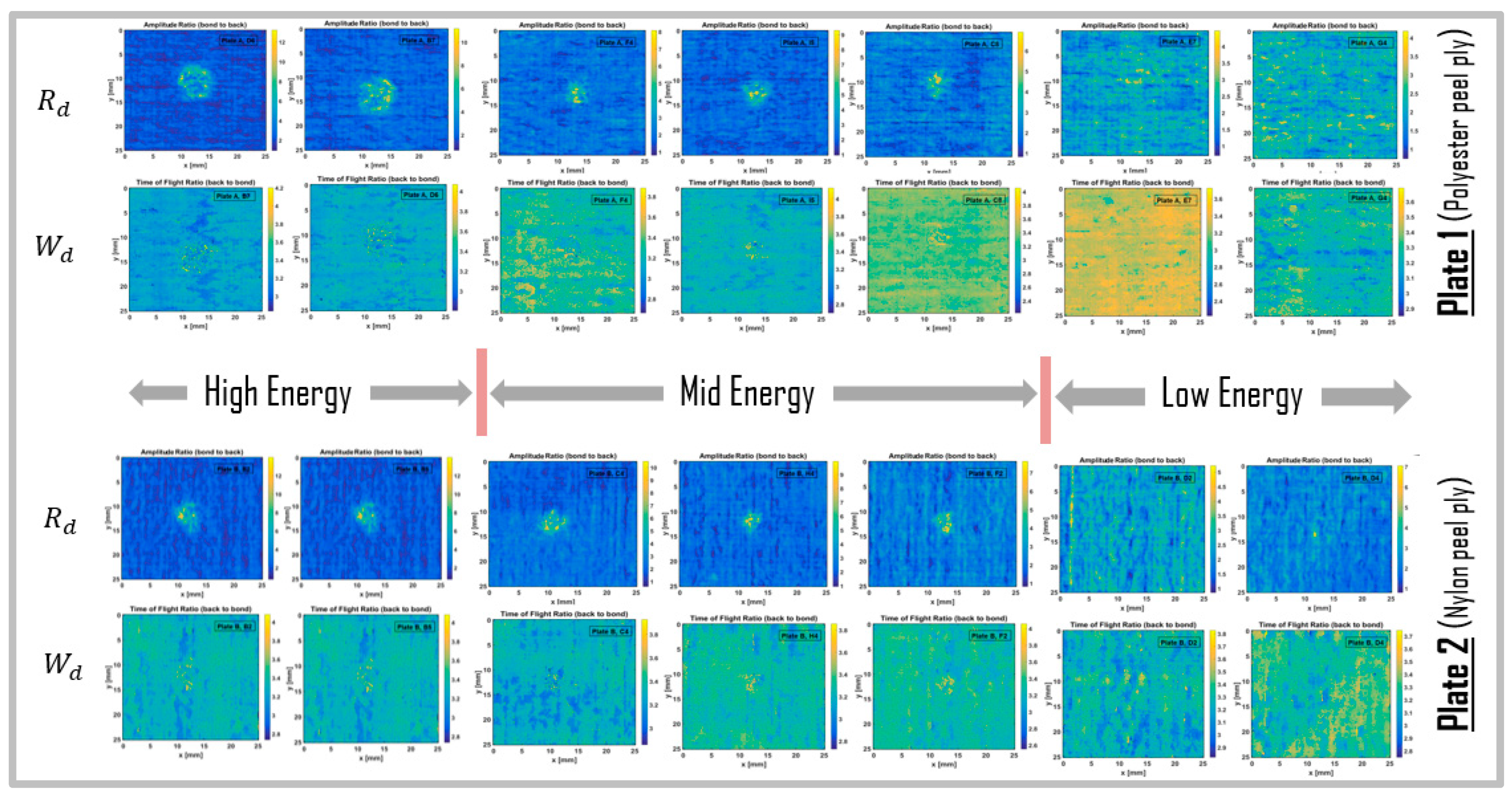
Figure 8.
(a) A newly proposed Energy vs. Damage size curve for Plate 1 (polyester peel ply) and Plate 2 (nylon peel ply) obtained from SAM analysis data. (b) A newly proposed BQI vs. Energy curve for Plate 1 (polyester peel ply) and Plate 2 (nylon peel ply) obtained from SAM analysis data. The graph shows that the bond in Plate 1 was stronger than Plate 2.

Figure 9.
(a) Scanning acoustic microscope, (b) schematics of the composite inspection and internal modules in SAM, (c) schematic of two Time of Flights (TOFs).
Figure 9.
(a) Scanning acoustic microscope, (b) schematics of the composite inspection and internal modules in SAM, (c) schematic of two Time of Flights (TOFs).
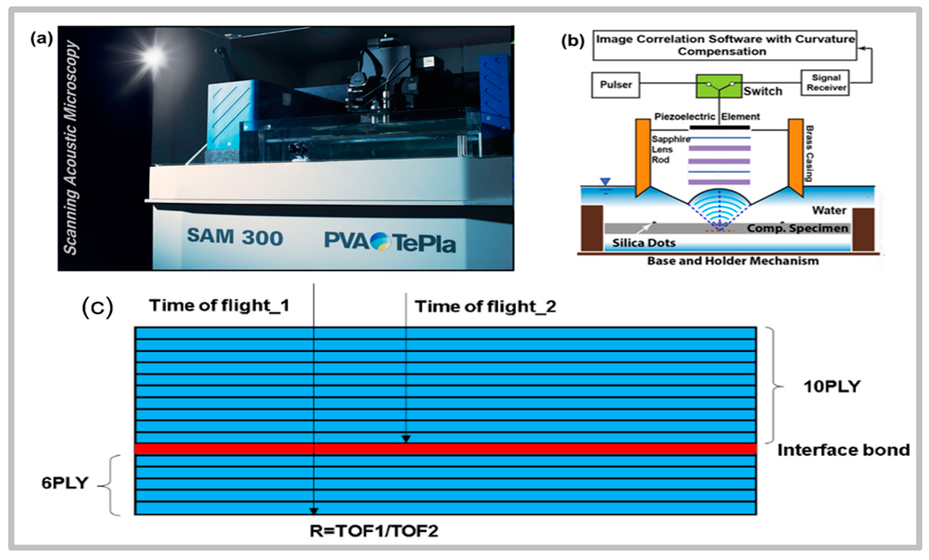
Figure 10.
Saved signals from two different locations on the plate.

Figure 11.
Distribution of TOFs from the bond line surface. (Top) Plate A, (bottom) Plate C, arranged according to the zones.
Figure 11.
Distribution of TOFs from the bond line surface. (Top) Plate A, (bottom) Plate C, arranged according to the zones.

Figure 12.
Distribution of , i.e., TOF ratios of the bottom surface to the bond line. (Top) Plate A, (bottom) Plate C. The red arrow shows an existing defect during manufacturing and thus these areas were avoided during the analysis.
Figure 12.
Distribution of , i.e., TOF ratios of the bottom surface to the bond line. (Top) Plate A, (bottom) Plate C. The red arrow shows an existing defect during manufacturing and thus these areas were avoided during the analysis.

Figure 13.
Probability density function of the Time-of-Flight ratios obtained from Plate A and C (left). (Right) The same ratios and their respective deviations between Plate A and Plate C are indicated for each zone that is identified in Figure 11. Please note that the red and blue dotted lines show the mean values of the distributions.

Figure 14.
SAM scan result for Plate A showing delamination or debonding with red on a green background.
Figure 14.
SAM scan result for Plate A showing delamination or debonding with red on a green background.
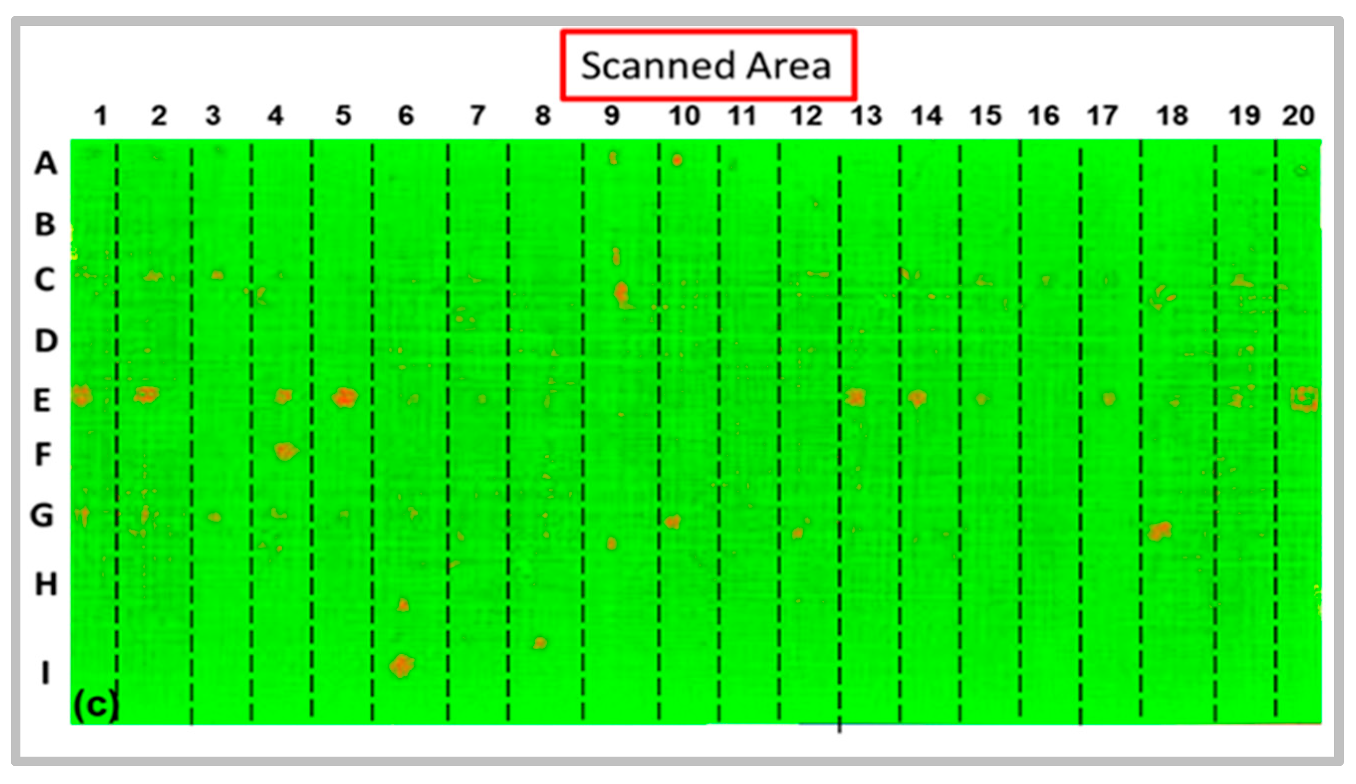
Figure 15.
SAM scan result for Plate C showing delamination or debonding with red on a green background.
Figure 15.
SAM scan result for Plate C showing delamination or debonding with red on a green background.
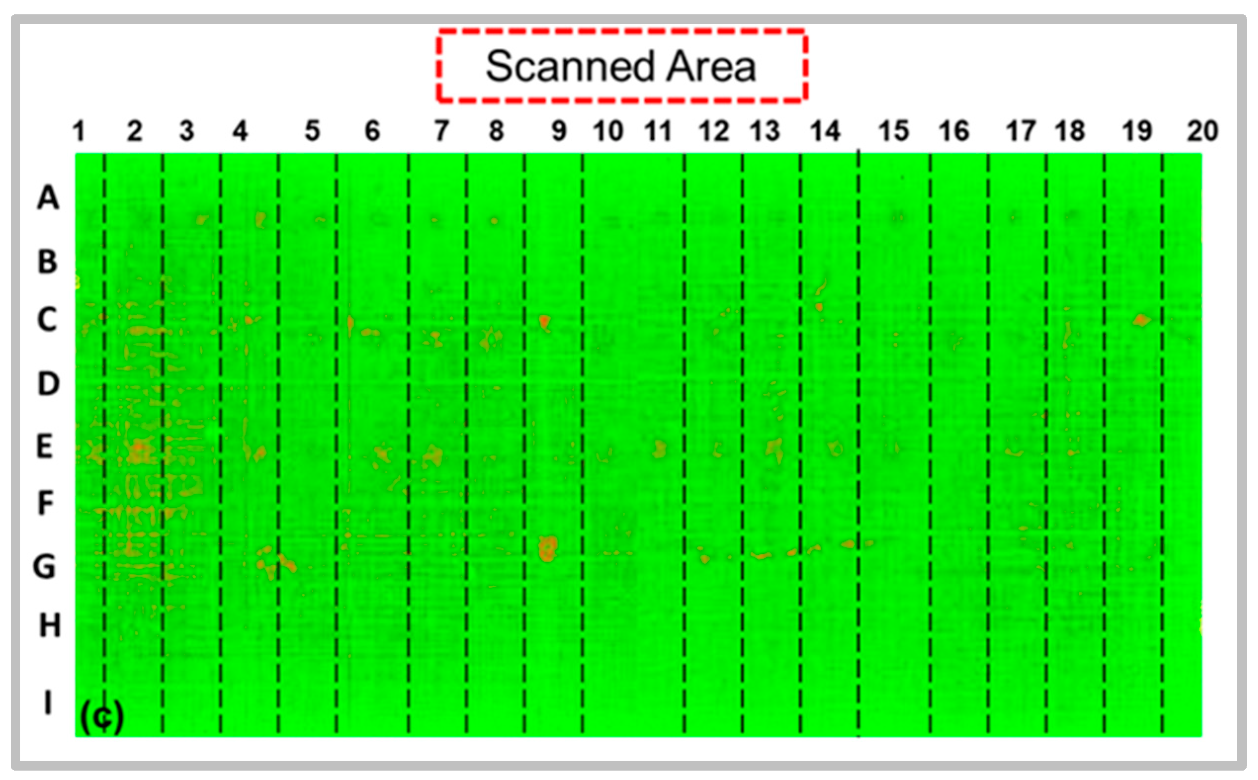
Figure 16.
Regions of Plate A showing debonding or delamination as affected by the various levels of impact energy. Color bars indicate the signal loss factors. The higher the loss, the redder the image will become. Thus, blue indicated a higher reflection amplitude of the ultrasound signal.
Figure 16.
Regions of Plate A showing debonding or delamination as affected by the various levels of impact energy. Color bars indicate the signal loss factors. The higher the loss, the redder the image will become. Thus, blue indicated a higher reflection amplitude of the ultrasound signal.

Figure 17.
Regions of Plate C showing debonding or delamination as affected by the various levels of impact energy. Color bars indicate signal loss factors. The higher the loss, the redder the image will become. Thus, blue indicated a higher reflection amplitude of the ultrasound signal.
Figure 17.
Regions of Plate C showing debonding or delamination as affected by the various levels of impact energy. Color bars indicate signal loss factors. The higher the loss, the redder the image will become. Thus, blue indicated a higher reflection amplitude of the ultrasound signal.

Figure 18.
Energy vs. Damage diameter for Plate A and Plate C.

Figure 19.
BQI vs. impact energy for Plate A and Plate C.

Disclaimer/Publisher’s Note: The statements, opinions and data contained in all publications are solely those of the individual author(s) and contributor(s) and not of MDPI and/or the editor(s). MDPI and/or the editor(s) disclaim responsibility for any injury to people or property resulting from any ideas, methods, instructions or products referred to in the content. |
© 2024 by the authors. Licensee MDPI, Basel, Switzerland. This article is an open access article distributed under the terms and conditions of the Creative Commons Attribution (CC BY) license (https://creativecommons.org/licenses/by/4.0/).
Share and Cite
MDPI and ACS Style
Banerjee, S.; Tavaf, V.; Indaleeb, M.M. Ultrasonic Nondestructive Evaluation of Composite Bond Strength: Quantification through Bond Quality Index (BQI). J. Compos. Sci. 2024, 8, 107. https://doi.org/10.3390/jcs8030107
AMA Style
Banerjee S, Tavaf V, Indaleeb MM. Ultrasonic Nondestructive Evaluation of Composite Bond Strength: Quantification through Bond Quality Index (BQI). Journal of Composites Science. 2024; 8(3):107. https://doi.org/10.3390/jcs8030107
Chicago/Turabian StyleBanerjee, Sourav, Vahid Tavaf, and Mustahseen M. Indaleeb. 2024. "Ultrasonic Nondestructive Evaluation of Composite Bond Strength: Quantification through Bond Quality Index (BQI)" Journal of Composites Science 8, no. 3: 107. https://doi.org/10.3390/jcs8030107