
Numerical Simulation of Transverse Crack on Composite Structure Using Cohesive Element
by
 ,
,
Heri Heriana
, 
Rebecca Mae Merida Catalya Marbun
,
Bambang Kismono Hadi
*,
Djarot Widagdo
and
Muhammad Kusni
Mechanics of Solid and Lightweight Structures Research Group, Faculty of Mechanical and Aerospace Engineering, Institut Teknologi Bandung, Jl. Ganesha 10, Bandung 40132, Indonesia
*
Author to whom correspondence should be addressed.
J. Compos. Sci. 2024, 8(4), 158; https://doi.org/10.3390/jcs8040158
Submission received: 4 February 2024
/
Revised: 7 April 2024
/
Accepted: 18 April 2024
/
Published: 22 April 2024
(This article belongs to the Section Composites Modelling and Characterization)
Abstract
:Due to their anisotropic behavior, composite structures are weak in transverse direction loading. produces transverse cracks, which for a laminated composite, may lead to delamination and total failure. The transition from transverse crack to delamination failure is important and the subject of recent studies. In this paper, a simulation of transverse crack and its transition to delamination on cross-ply laminate was studied extensively using a cohesive element Finite Element Method (FEM). A pre-cracked [0/90] composite laminate made of bamboo was modeled using ABAQUS/CAE. The specimen was in a three-point bending configuration. Cohesive elements were inserted in the middle of the 90° layer and in the interface between the 0° and 90° layer to simulate transverse crack propagation and its transition to delamination. A load–displacement graph was extracted from the simulation and analyzed. As the loading was given to the specimen, stress occurred in the laminates, concentrating near the pre-cracked region. When the stress reached the tensile transverse strength of the bamboo, transverse crack propagation initiated, indicated by the failure of transverse cohesive elements. The crack then propagated towards the interface of the [0/90] laminates. Soon after the crack reached the interface, delamination propagated along the interface, represented by the failure of the longitudinal cohesive elements. The result of the numerical study in the form of load–displacement graph shows a consistent pattern compared with the data found in the literature. The graph showed a linear path as the load increased and the crack propagated until a point where there was a load-drop in the graph, which showed that the crack was unstable and propagated quickly before it turned into delamination between the 0o and 90° plies.
1. Introduction
In recent years, composite material has been vastly used in many engineering industries due to its enhanced property (high strength and specific stiffness, durability, corrosion resistant, etc.) and weight reduction potential, among other exceptional advantages [1,2,3]. However, the analysis of strength and failure mechanism of a composite is more complex than that of isotropic materials due to its inhomogeneous and anisotropic nature. There are several factors affecting the properties of composite materials, making the strength analysis and the failure modes more complex. Sometimes, more than one failure mode will appear and interact before the material comes into a complete failure [4]. One of the factors which significantly affects the strength and damage mechanism of a composite’s structure is the direction of fiber.
The strength of a unidirectional composite lamina lies in its fiber direction or longitudinal direction. In the transverse direction, however, the composite material is weak since there is no fiber reinforcement contribution in this direction. The strength in the transverse direction is determined mostly by the strength of the matrix and fiber–matrix bonding. For a multidirectional composite laminate, failure usually starts at the ply enduring the transverse load [5]. Failure due to transverse loading usually starts either with matrix transverse crack or fiber–matrix debonding. Transverse crack could propagate and induce delamination in the interface between plies. Delamination (or interface debonding) is one of the most common and anticipated failure modes on composite structures. Normally, it is caused by the interaction of normal stress with shear stress, but it could also be caused by other failure modes such as transverse crack, low-velocity impact, fatigue, or manufacturing flaws [6,7,8].
Predicting transverse crack and delamination is crucial. Composites have a tendency as a brittle material, making a crack initiate and propagate quickly [4]. Delamination could happen in a relatively low loading, and it is very hard to detect since it happens between layers. It could also cause a significant degradation of the overall load-bearing capabilities. Finite element analysis is one of the reliable tools to analyze structural response and mechanism due to loadings, including crack propagation and delamination. One of the tools that is commonly be used to analyze the propagation of a crack is cohesive elements [6,7], also used to model responses in adhesively bonded interface. A cohesive element is normally designed to represent the separation at the zero-thickness interface between layers by combining material strength and fracture mechanics concepts to identify the failure phenomenon [9,10].
The cohesive element was developed from a proposition developed by Dugdale and Barrenblatt [11,12]. The proposition assumes that there is a process zone ahead of the crack tip which undergoes a softening response before crack occurs. Within this zone, opening is resisted by cohesive tractions. It is then known that the absorbed energy before the zone finally opens is equal to the fracture energy of the materials. The cohesive zone was firstly implemented in finite element analysis to simulate concrete cracking by Hillenborg [13], and has been widely developed up to this day.
Cohesive elements relate stresses in material in terms of surface traction with the relative displacement between adjacent nodes using Traction–Separation Law [14]. This law links the bulk material property to fracture characteristics of the material [15]. Thus, a cohesive element method is characterized by the properties of the bulk material, the crack initiation condition, and the crack evolution function [16].
The objective of this work is to utilize cohesive elements in modeling transverse crack propagation and its transition to delamination in the interface of a cross-ply composite laminate. Analysis of load–displacement graphs will also be presented to better expand the understanding about the mechanism of transverse crack propagation and its transition to delamination. A comparison between two specimens with different spans will also be presented to give insights about the effect of geometry factors (in this case, the span of a beam) to the bending response of the overall structure, before and after transverse crack and delamination.
In this paper, a bamboo specimen was used to model the transverse crack since bamboo is widely available and has a natural unidirectional fiber composite. The specimen consists of two parts. The bottom part has a 90° fiber direction, where the fiber is in the transverse, thickness direction, while the upper part has a 0° fiber direction, where the fiber is in the longitudinal, span direction. The bottom and the upper parts were glued together with PVAc adhesive. Three-point bending was applied to the specimen and an initial crack was produced in the bottom part to start the transverse crack. The mechanical behavior of the bamboo is given in [17,18,19], while the properties of PVAc are given in [20,21], and the Mode I fracture toughness of bamboo is given in [22].
2. Cohesive Element
2.1. Traction–Separation Law
As mentioned before, cohesive elements’ modeling adopts Traction–Separation Law to predict microstructural failure within an element. This law correlates traction happening in the element interface with the relative displacement of adjacent nodes in the cohesive elements. Based on this law, when loading is given to the element, there will be a relative displacement between the adjacent nodal of the element. As the loading continues, traction in the element grows larger until reaching a predetermined maximum traction number where damage to the element is initiated. After the maximum traction is reached, damage develops in the cohesive element, indicated by the degradation of stiffness, before it finally comes into a complete failure. The degradation of cohesive elements’ stiffness is known as the softening response.
The traction and relative displacement in the cohesive element were modeled in several constitutive equations, as shown in Figure 1. The Bilinear—also called the linear elastic–linear softening—model is one of the simplest models. This model is also the default model of the Traction–Separation Law used in ABAQUS/CAE [23]. The maximum nominal stress of the graph links to the interfacial strength of the cohesive element (in this case, the tensile transverse strength) and the area under the Traction–Separation model equals the fracture energy of the material. The response of the cohesive element to loading according to Traction–Separation Law is well explained by C. G. Davilla [24].
Figure 2 shows a detailed illustration of the cohesive element responses to loading P. The slope of the bilinear equation before maximum traction (point 0-1-2) represents the initial stiffness of the cohesive element, Kp. It is a numerical value rather than one obtained from experiment. Several studies have been conducted to determine the ideal number for this parameter. Point 2 represents the maximum allowable traction of the cohesive elements. This point corresponds to the interfacial strength of the material being represented by the cohesive elements. The underlying constitutive equation for the linear range is given by Equation (1):
The slope after the maximum stress (point 2-3-4) characterizes the rate of degradation of the cohesive element stiffness. After the maximum traction is reached, the cohesive elements will undergo a softening response where the penalty stiffness Kp will be degraded. The underlying constitutive equation for the softening response is given by Equation (2):
where D is the scalar damage variable ranging from 0 to 1, where 0 means no damage and 1 means complete failure.
The cohesive element undergoes a softening response until it comes into a complete failure (point 4). In the softening process, damage accumulates at the interface of the elements and the interface only bears a loading below . The energy released when the element reached point 3 is the area of the triangle 0-2-3. Point 4 represents the critical value of the energy release of the cohesive element. This value corresponds to the fracture energy of the material. Cohesive elements do not carry any tensile or shear stress above point 4. In other words, point 4 is where the cohesive elements come to a complete failure (all of the available interfacial fracture energy has been consumed). At this point, Kp is zero and the cohesive element no longer bear any loads. Any loadings after point 4 are no longer carried by the cohesive element since it no longer has stiffness (point 5).
The area under the traction–separation curve relating to fracture energy can also be calculated using Equation (3):
The integration suggests that for an assumed shape of curve, the stress at initiation, and displacement at failure can be set such that the energy absorbed per unit cracked area is equal to the material’s critical failure energy.
Simulation using cohesive elements is very sensitive to the size of the mesh. Few elements will result in an inaccurate representation of traction ahead of the crack tip region. There are several studies that have been conducted to establish the minimum number of elements. Turon suggested that a minimum of three cohesive elements in the processing zone is sufficient to conduct a successful FEM simulation [15].
2.2. Numerical Parameters
There are three parameters needed to be defined for the cohesive elements to satisfy the traction–separation calculation: cohesive stiffness, damage initiation, and damage evaluation. Since the cohesive stiffness is a numerical value, choosing the initial stiffness should be carefully considered because the success of the simulation depends on the determination of this number. Several values have been proposed for this numbers, but for this paper, the initial stiffness of 106 N/mm2 was chosen based on Da Villa’s experiment [24].
Damage initiation refers to the beginning of the degradation of the cohesive element. It occurs when a prespecified maximum stress or strain value as the damage initiation criteria is reached [23]. Several criteria are provided by ABAQUS/CAE as the initial damage criteria. In this study, the MAXS damage initiation criteria were chosen. ,, and represent the nominal maximum nominal stress tensors specified for the criteria. Damage is assumed to begin when the maximum nominal stress ratio (as defined in the expression below) reaches a value of one, as represented by the function in Equation (4):
where
Damage evolution refers to the rate of stiffness degradation after the damage initiation criterion is surpassed. It is specified by displacement or energy control. In this criterion, the fracture energy Gc of each material (bamboo and PVAc) is used to define the damage evolution criteria for each cohesive element.
3. Numerical Models
3.1. Materials and Geometries of Laminates
As mentioned before, Gigantochloa apus bamboo was used as the subject of this study. It has unidirectional fibers with appropriate thickness to observe crack propagation. There are two models simulated in this study, a short-span beam with a dimension of 20 × 10 × 8 mm, and a long-span beam with the dimension of 42 × 10 × 8 mm. The long-span beam is based on ASTM D5045 [19] for three-point bending specimens. In the middle of the bottom, 90° layer, a 2 mm notch is introduced to the specimen to represent the initial crack. The laminates are staged in a three-point bending configuration to support a plane-bending load. The loading speed is set to 1 mm/min. Figure 3 shows the dimension and configuration of each specimen, while Table 1 sums up all the specimen dimensions.
3.2. Material Properties
3.3. Numerical Models and Procedures
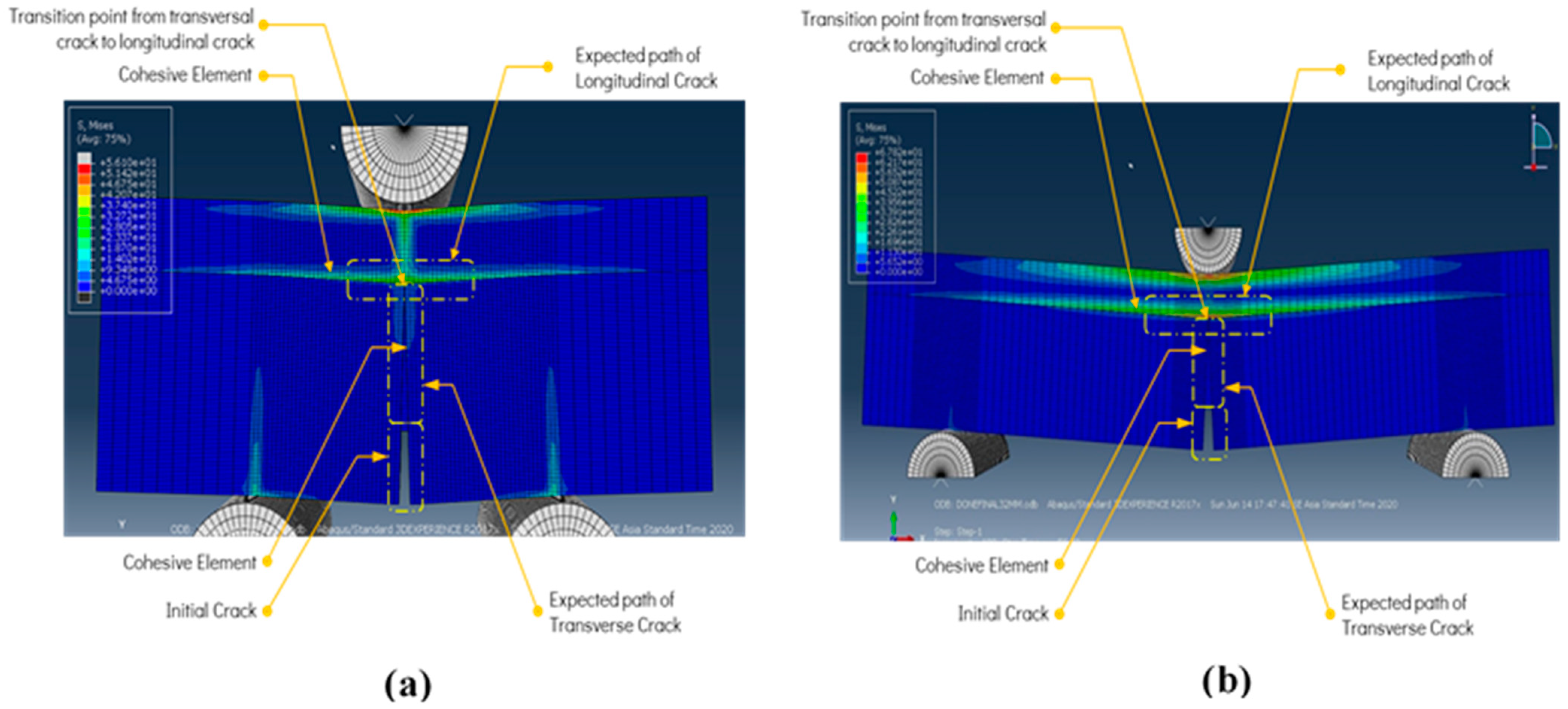
Since the geometry and size are relatively simple, the model was constructed directly on ABAQUS/CAE. The results are given in Figure 4 and Figure 5 for the short and long beams, respectively. Data from Table 2 and Table 3 were used to define the material and cohesive element. Cohesive elements are inserted in the middle of the bottom layer and in between the 0° and 90° layers. For the cohesive element inserted in the middle of the 90° layer, the parameters used to define the cohesive element are the strength and fracture energy of the bamboo. Therefore, cohesive elements can be considered part of the bamboo and will represent the response of bamboo’s 90° layer to loadings, particularly the propagation of the transverse crack. For the cohesive element in the interface zone, the parameters used the strength and fracture energy of PVAc adhesive; therefore, these will represent the response of PVAc adhesive to loading—in this case, a delamination.
The transversal cohesive element, longitudinal cohesive element, and initial crack are highlighted by yellow-dashed squares 1, 2, and 3, respectively, in both specimens shown in Figure 4 and Figure 5.
In the FEM model, orientation was defined to the specimen according to the coordinate system to distinguish the 0° and 90° layer. A local coordinate system was preset to the material so that x(+) was the 0° direction. General surface-to-surface was used to define contact interaction between specimens with pin or stands. The pin was given a roll constraint, and the pin impactor was set to have vertical axis movement only. An automatic stabilization parameter was used to help the calculation on ABAQUS/CAE smoother and faster to reach convergence. This parameter was used because a simulation involving the failure of materials (in terms of crack propagation for this study) is often unstable and a convergence result is difficult to reach.
4. Results and Discussion
4.1. Simulation Results of Short and Long Beams
There are two specimens modeled in this study (short beam and long beam) differing in the span of the specimen. The two models showed similar damage characteristics. As the load was applied, stress occurred in the structure and concentrated near the initial cracked region. Tensile stress dominated in the bottom ply of the laminate in the transverse direction of the composite specimens. The stress kept increasing until it finally reached the transverse tensile strength of the bamboo, which was predefined as the damage initiation criteria for the transverse cohesive element. The stress caused a degradation in stiffness and eventually fell into a complete failure, representing crack propagation in the specimen.
The crack propagated in a stable manner towards the laminates interface. When the crack reached its critical length, the crack became unstable and propagated quickly before coming into a halt when reaching the interface zone. At this stage, the crack had divided the bottom ply into two totally separate parts; hence, it can be said that the 90° layer had failed. Figure 6 shows the stress distribution in the composite structures at the time transverse crack reached the interface. The minimum distribution of stress in the 90° layers confirms the failure of the 90° layer.
The longitudinal cohesive elements are now the focus points. Due to the failure of the bottom layer, the stress was then sustained by the upper layer (0° layer). The normal stress occurring in the upper ply was parallel to the direction of the ply’s fiber. As the loading from the pin continued, shear stress was introduced to the interface of the [0/90] laminates. When the shear stress reached the adhesive shear strength, the longitudinal cohesive elements experienced stiffness degradation before it completely failed, indicating the initiation of delamination. Further loading showed what happened after delamination occurred, that was, the delamination propagated along the interface. Figure 6 shows the visualization of the cohesive element’s failure (red zones).
4.2. Load–Displacement Graph Analysis
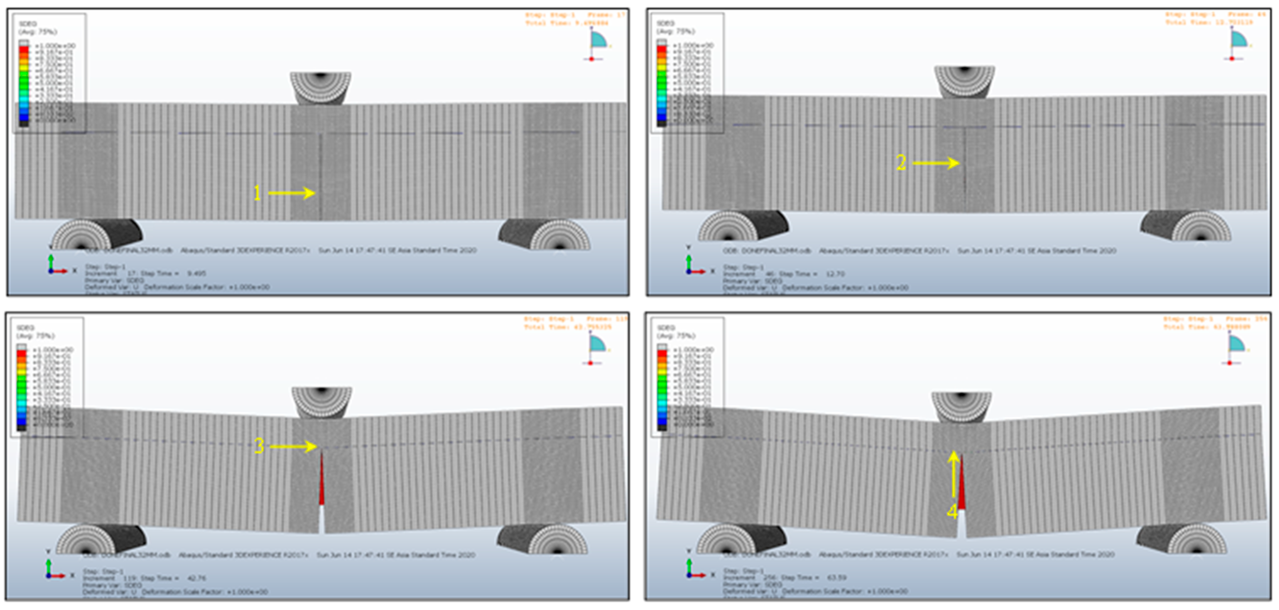
Figure 7a,b shows the load–displacement graph (P − δ) simulation for short beam and long beam, respectively. This graph correlates the reaction force exerted by the impactor pin as a reaction from the specimen with pin displacement. As previously mentioned, the simulation began when the pin gave a loading to the specimen. As a response to this loading, normal stress emerged in the specimen and increased as the pin moved down. This response was recorded in the load–displacement graph, following a linear path. Point 1 in Figure 7 marks the point when the transverse crack propagation began. Since the crack was still small, the specimen could still bear the load, indicated by the increasing loading in the load–displacement graph. The graph kept going up and the crack kept propagating until it reached its critical length (point 2). At this point, the crack turned unstable and propagated quickly towards the interface of the laminate before it stopped. This incident is denoted by a sudden load-drop in the load–displacement graph (point 2–3). The load-drop indicates there is a rapid energy release when the structure fails. The transverse crack stopped when it reached the interface of the laminate. This point is depicted as the bottom valley of the load–displacement graph (point 3). It was then determined that the 90o layer had failed.
After the 90° layer failed, the loading was then carried by the 0° layer (the upper ply of the laminates). There was a recovery in the load–displacement graph since the loading was now accounted by 0° layer. The tension/compression stress was now parallel to the direction of the fiber. The load–displacement graph formed another linear relation after the load-drop (point 3–4). Delamination due to shear stress was initiated when the graph was still inclining upward, marked at point 4. Figure 8 and Figure 9 show the cohesive element’s failure, representing transverse crack propagation and its transition to delamination for the case of the short and long beams, respectively.
Figure 10 below shows that the delamination occurs on the interface of the laminate for both the short and long beams. The delamination is represented by the red zone in the longitudinal cohesive elements (in this case, modeling the PVAc layer), indicating that the elements failed completely.
To validate the load–displacement graph results from this numerical study, a comparison was made with the experimental results on a similar study of cross-ply laminate conducted by Wafai et al. [5]. In their study, a glass-fiber polypropylene cross-ply composite laminate was tested under a three-point bending configuration. Their results showed a similar pattern to our numerical results.
Load–displacement graphs represent the response of a structure with a certain characteristic (dimension and properties) due to the bending load. The characteristic of the structure is manifested in the gradient of the load–displacement graph. Structures with different geometry or material properties will have different load–displacement gradients. The steeper the gradient, the more difficult it is for the structures to deflect due to the bending moment.
Figure 11 shows the comparison of the load–displacement graph between the short and long beams, showing how the span of a structure would give different responses to bending. Figure 12 and Figure 13 show the comparison of the gradients of both specimens before and after load-drop.
Table 4 shows the comparisons of gradients for both specimens.
The linear graph before load-drop characterizes the response of the [0°/90°] laminates of each specimen to the bending load. The load-drop itself represents the transition of the structure’s configuration of bearing the bending load from [0°/90°] to only [0°]. The transition of the load-bearing structure from [0/90] to only the [0] layer when the crack reached the interface zone was captured as the load-drop in the load–displacement graph. Consequently, the linear graph after load-drop characterizes the response of the remaining [0°] bearing the load. Table 4 gives us further information. First, the gradient of the short beam is always greater than that of the long beam. Second, it is shown that the gradients after the load-drop are always smaller than the gradients before the load-drop. These facts denote that structure configuration, in this case span and thickness, governs the response of a structure to the bending load.
The gradient of the load–displacement graph of a structure is governed by Equation (5):
From the formulation, it can be seen that the response of a structure to the bending load is determined by the properties of the laminates (manifested in the bending stiffness) and the geometry of the specimen (span, width and thickness). Moreover, span and thickness play a significant part in determining the stress occurred within a specific ply in a composite structure due to a specific loading. The conversion of the specimen thickness from 8 mm to 2 mm for both the short and long beams gives a prominent effect to the structure. The alteration to the 0° layer also gives a notable effect to the overall structure bending stiffness. Both factors would significantly affect the response of the structure to the bending load; hence, the gradient decreases.
Table 4 also shows that there was a steeper decline in the slope of the load–displacement graph of the long beam than the decline in the short beam slope. This shows that the conversion of load-bearing structures from [0/90] laminates to only [0] lamina affects the long beam specimen more than it affects the short beam specimen. From this result, it can be deduced that structures with wider spans will be affected more if failure occurs to one of the layers of ply than structures with a shorter span. Structures with larger deformation would be more likely to deform more easily when a layer of ply failed.
4.3. Comparison of Load-Deformation Graph in the Delamination
Table 5 shows a comparison of load and pin displacement from each crucial point happening in the specimen. In the table, we can see that a bigger loading is needed to initiate crack propagation and delamination in the short beam. From the table, it can be concluded that the amount of normal stress occurring in a structure is directly proportional to the span of a structure. In other words, for the same structure with the same geometry, and properties, the same loading may generate a bigger stress to the structure with a bigger span, making it more prone to failure due to the bending load. This happens because the span of the structure acts as the moment arm to the bending load, generating a bigger stress for the same loading.
5. Conclusions
A transverse crack and its transition to longitudinal crack (commonly named delamination) on composite structures is simulated using finite element analysis by means of cohesive elements. The propagation of the transverse crack and its transition to delamination is represented by the failure of cohesive elements. A composite bamboo of [0/90] laminates is modeled in a three-point bending configuration. Cohesive elements are inserted in the mid-plane of the bottom ply of the laminate (the [90] layer) as part of the bamboo specimen and in the interface of the [0/90] laminate to represent adhesive layers (PVAc glue). The properties of bamboo and adhesive are defined for the cohesive element; so, each represents the behavior of the corresponding material.
Crack propagation and delamination are represented by the failure of cohesive elements. The strength of the material and damage mechanics parameters are pre-defined for the cohesive element as damage initiation and evolution criteria. Once the damage initiation criteria are reached, the cohesive elements undergoes a softening response and came into a complete failure. The failure of the cohesive elements is visualized by ABAQUS/CAE by the red color of the damaged elements. The crack propagates in a stable manner, which swiftly changes into unstable propagation when the crack length reaches its critical value. The cracks propagate towards the interface of the laminate. Delamination occurs when the damage initiation criteria of the adhesive are reached, and further simulation indicates the delamination develops along the interface. The load–displacement graph extracted from the simulation gives a more detailed representation of the phenomena happening throughout the simulation.
Author Contributions
H.H. provided administration, R.M.M.C.M. wrote the first draft and did the FEM analysis, B.K.H. chaired the research, conceptualization and wrote the final manuscript, D.W. and M.K. did the analysis. All authors have read and agreed to the published version of the manuscript.
Funding
This work was supported by the P2MI scheme from the Lighweight Structures Research Group, Faculty of Mechanical and Aerospace Engineering, Institut Teknologi Bandung for the year of 2022. The authors would like to thank the Institut for the generous funding.
Data Availability Statement
Full data is available upon request.
Conflicts of Interest
The authors declare no conflicts of interest.
References
- Rivallant, S.; Bouvet, C.; Hongkarnjanakul, N. Faulire Analysis of CFRP laminates subjected to compression after impact: FE simulation using discrete interface elements. Compos. Part A Appl. Sci. Manuf. 2013, 55, 83–93. [Google Scholar] [CrossRef]
- Farrokhabadi, A.; Bahrami, M.; Babaei, R. Predicting the matrix cracking formation in symmetric composite laminates. Compos. Struct. 2019, 223, 110945. [Google Scholar] [CrossRef]
- Wimmer, G.; Shuecker, C.; Peterman, H. Numercal Simulation of Delamination Onset and Growth in Laminated Composite. E-J. Nondestruct. Test. 2006. Available online: https://www.researchgate.net/profile/Clara-Schuecker/publication/228413566_Numerical_simulation_of_delamination_onset_and_growth_in_laminated_composites/links/02e7e52ef86ad04b11000000/Numerical-simulation-of-delamination-onset-and-growth-in-laminated-composites.pdf (accessed on 23 January 2022).
- Hallet, S.; Harper, P. Modeling Delamination with Cohesive Interface Elements. In Numerical Modeling of Failure in Advanced Composite Materials; Woodhead Publishing: Sawston, UK, 2015; pp. 55–72. [Google Scholar]
- Wafai, H.; Yudhanto, A.; Lubineau, G.; Yaldiz, R.; Verghese, N. An experimental approach that assesses in-situ micro-scale damage mechanisms and fracture toughness in thermoplastic laminates under out-of plane loading. Compos. Struct. 2019, 207, 546–559. [Google Scholar] [CrossRef]
- Saeedifar, M.; Fotouhi, M.; Najafabadi, M.A. Prediciton of delamination growth in laminated composites using acoustic emmision and cohesive zone modeling techniques. Compos. Struct. 2015, 124, 120–127. [Google Scholar] [CrossRef]
- Elmarakbi, A.; Hu, N.; Fukunaga, H. Finite element simulation of delamination growth in composite materials using LS-DYNA. Compos. Sci. Technol. 2009, 69, 2383–2391. [Google Scholar] [CrossRef]
- Kashtalyan, M.; Soutis, C. The effect of delaminations induced by transverse cracks and splits on stiffness properties of composite laminates. Compos. Part A Appl. Sci. Manuf. 2000, 31, 107–119. [Google Scholar] [CrossRef]
- Gibson, R.F. Principles of Composite Material Mechanics; McGraw-Hill, Inc.: New York, NY, USA, 1994. [Google Scholar]
- Davilla, C.G.; Camanho, P.P.; Turon, A. Effective Simulation of Delamination in Aeronautical Structures Using Shells and Cohesive Elements. J. Aircr. 2008, 45, 663–672. [Google Scholar] [CrossRef]
- Dugdale, D. Yielding of Steel Sheest Containing Slits. J. Mech. Phys. Solids 1960, 8, 100–104. [Google Scholar] [CrossRef]
- Barrenblatt, G. The Mathematical Theory of Equilibrium Crack in Brittle Fracture. Adv. Appl. Mech. 1962, 7, 55–129. [Google Scholar]
- Hillerborg, A.; Modeer, M.; Peterson, P. Analysis of Crack Formation and Crack Growth in concrete by means of fracture mechanics and finite elements. Cem. Concr. Res. 1976, 6, 773–781. [Google Scholar] [CrossRef]
- Costa, M.; Viana, G.; Créac’Hcadec, R.; Da Silva, L.F.M.; Campilho, R.D.S.G. A cohesive zone element for mode I modelling of adhesives degraded by humidity and fatigue. Int. J. Fatigue 2018, 112, 173–182. [Google Scholar] [CrossRef]
- Turon, A.; Davila, C.G.; Camanho, P.P.; Costa, J. An Engineering Solution for Mesh Size Effects in the simulationof delamination using cohesive zone model. Eng. Fract. Mech. 2007, 74, 1665–1682. [Google Scholar] [CrossRef]
- Gheibi, M.R.; Shojaeefard, M.H.; Googarchin, H.S. Direct Dtermination of A New Mode-Dependent Cohesive Zone Model to Simulate Metal-to-Metal Adhesive Joints. J. Adhes. 2018, 95, 943–970. [Google Scholar] [CrossRef]
- Hadi, B.K.; Subadra, A.; Kuswoyo, A. Mechanical Properties of Natural Bamboo Due to Tensile and Compression Loadings. Key Eng. Mater. 2018, 775, 576–581. [Google Scholar] [CrossRef]
- Liu, P.; Zhou, Q.; Jiang, N.; Zhang, H.; Tian, J. Fundamental research on tensile properties of phyllostachys bamboo. Results Mater. 2010, 7, 100076. [Google Scholar] [CrossRef]
- “What are the Mechanical properties of Bamboo”, Bamboo Import. Available online: https://www.bambooimport.com/en/what-are-the-mechanical-properties-of-bamboo (accessed on 13 January 2022).
- Qiao, L.; Easteal, A.J. Aspects of the performance of PVAc adhesives in wood joints. Pigment. Resin Technol. 2001, 30, 79–87. [Google Scholar] [CrossRef]
- Khan, U.; May, P.; Porwal, H.; Nawaz, K.; Coleman, J.N. Improved Adhesive Strength and Toughness of Polyvinyl Acetate Glue on Addition of Small Quantities of Graphene. ACS Appl. Mater. Interfaces 2013, 5, 1423–1428. [Google Scholar] [CrossRef] [PubMed]
- Chen, Q.; Dai, C.; Fang, C.; Chen, M.; Zhang, S.; Liu, R.; Liu, X.; Fei, B. Mode I interlaminar fracture toughness behavior and mechanisms of bamboo. Mater. Des. 2019, 183, 108132. [Google Scholar] [CrossRef]
- ABAQUS. Analysis User’s Manual; Version 6.12; Dassault Systemes Simulia, Inc.: Johnston, RI, USA, 2012. [Google Scholar]
- Davila, C.; Camanho, P.; de Moura, M. Mixed-mode Decohesion Elements For Analyses of Progressive Delamination. In Proceedings of the 19th AAIA Aerodynamics Conference, Anaheim, CA, USA, 11–14 June 2001. [Google Scholar]
Figure 1.
Various constitutive equation of Traction–Separation Laws. (a) Bi-linear. (b) Non-Linear softening. (c) Trapezoidal. (d) Exponential.
Figure 1.
Various constitutive equation of Traction–Separation Laws. (a) Bi-linear. (b) Non-Linear softening. (c) Trapezoidal. (d) Exponential.

Figure 2.
Traction-Separation mechanism on cohesive elements.

Figure 3.
Specimen configurations (a) Short beam. (b) Long beam.

Figure 4.
Model simulations for short beam. (a) Full model. (b) Cohesive element. (c) Initial crack.
Figure 4.
Model simulations for short beam. (a) Full model. (b) Cohesive element. (c) Initial crack.

Figure 5.
Model simulations for long beam (a). Full model (b) Cohesive element. (c) Initial crack.

Figure 6.
Stress distribution in the specimen after the 90o layer failed. (a) Short beam. (b) Long beam.
Figure 6.
Stress distribution in the specimen after the 90o layer failed. (a) Short beam. (b) Long beam.

Figure 7.
Load–displacement graph (a) Short beam. (b) Long beam.

Figure 8.
Delamination visualization of short beam.

Figure 9.
Delamination visualization of long beam.

Figure 10.
Delamination visualization. (a) Short beam. (b) Long beam.

Figure 11.
Load–displacement graph comparison between short beam and long beam.

Figure 12.
Load–displacement graph gradient comparison before load-drop between short beam and long beam.
Figure 12.
Load–displacement graph gradient comparison before load-drop between short beam and long beam.

Figure 13.
Load–displacement graph gradient comparison after load-drop between short beam and long beam.
Figure 13.
Load–displacement graph gradient comparison after load-drop between short beam and long beam.


Table 1.
Specimens dimension.
| Length (mm) | Width (mm) | Height (mm) | |
|---|---|---|---|
| Short beam 0° | 20 | 10 | 2 |
| Short beam 90° | 20 | 10 | 6 |
| Long beam 0° | 42 | 10 | 2 |
| Long beam 90° | 42 | 10 | 6 |
Table 2.
Material properties for bamboo [17].
Table 2.
Material properties for bamboo [17].
| E11 (MPa) | E22 (MPa) | E33 (MPa) | v12 | v13 | v23 | G12 (MPa) | G13 (MPa) | G23 (MPa) |
|---|---|---|---|---|---|---|---|---|
| 29,028 | 5605 | 5605 | 0.3 | 0.3 | 0.3 | 28 | 28 | 28 |
| Thickness, t (mm) | Knn (N/mm2) | Kss (N/mm2) | Ktt (N/mm2) | τn (MPa) | τs (MPa) | τt (MPa) | Fracture Energy (10−6 J/mm2) | |
|---|---|---|---|---|---|---|---|---|
| Bamboo | 0.001 | 106 | 106 | 106 | 4.66 | 7 | 7 | 429 |
| PVAc | 0.001 | 106 | 106 | 106 | 14.5 | 14.5 | 14.5 | 200 |
Table 4.
Load–displacement gradient comparison.
| Short Beam | Long Beam | Unit | |
|---|---|---|---|
| Gradient P − δ graph Before load-drop | 638.31 | 163.69 | N/mm |
| Gradient P − δ graph After load-drop | 615 | 61.98 | N/mm |
| Δm | 23.31 | 101.71 | N/mm |
Table 5.
Load and displacement comparison between short beam and long beam.
| Short Beam | Long Beam | Units | |
|---|---|---|---|
| Pin displacement, initial crack propagation | 0.12 | 0.16 | mm |
| Load, initial crack propagation | 73.86 | 26.55 | N |
| Pin displacement, peak of load-drop | 0.22 | 0.20 | mm |
| Load, peak of load-drop | 131.41 | 30.13 | N |
| Pin Displacement, bottom of load-drop | 0.25 | 0.26 | mm |
| Load, bottom of load-drop | 110.36 | 16.48 | N |
| Pin displacement, delamination initiation | 0.48 | 1.06 | mm |
| Load, delamination initiation | 262.31 | 65.69 | N |
Disclaimer/Publisher’s Note: The statements, opinions and data contained in all publications are solely those of the individual author(s) and contributor(s) and not of MDPI and/or the editor(s). MDPI and/or the editor(s) disclaim responsibility for any injury to people or property resulting from any ideas, methods, instructions or products referred to in the content. |
© 2024 by the authors. Licensee MDPI, Basel, Switzerland. This article is an open access article distributed under the terms and conditions of the Creative Commons Attribution (CC BY) license (https://creativecommons.org/licenses/by/4.0/).
Share and Cite
MDPI and ACS Style
Heriana, H.; Marbun, R.M.M.C.; Hadi, B.K.; Widagdo, D.; Kusni, M. Numerical Simulation of Transverse Crack on Composite Structure Using Cohesive Element. J. Compos. Sci. 2024, 8, 158. https://doi.org/10.3390/jcs8040158
AMA Style
Heriana H, Marbun RMMC, Hadi BK, Widagdo D, Kusni M. Numerical Simulation of Transverse Crack on Composite Structure Using Cohesive Element. Journal of Composites Science. 2024; 8(4):158. https://doi.org/10.3390/jcs8040158
Chicago/Turabian StyleHeriana, Heri, Rebecca Mae Merida Catalya Marbun, Bambang Kismono Hadi, Djarot Widagdo, and Muhammad Kusni. 2024. "Numerical Simulation of Transverse Crack on Composite Structure Using Cohesive Element" Journal of Composites Science 8, no. 4: 158. https://doi.org/10.3390/jcs8040158