Optimal Clustering and Cluster Identity in Understanding High-Dimensional Data Spaces with Tightly Distributed Points

1
Living PlanIT AG, Knonauerstrasse 52E, 6330 Cham, Switzerland
2
Data Science Central, 2428 35th Avenue NE, Issaquah, WA 98029, USA
*
Author to whom correspondence should be addressed.
Mach. Learn. Knowl. Extr. 2019, 1(2), 715-744; https://doi.org/10.3390/make1020042
Submission received: 8 April 2019
/
Revised: 31 May 2019
/
Accepted: 3 June 2019
/
Published: 5 June 2019
(This article belongs to the Section Data)
Abstract
:The sensitivity of the elbow rule in determining an optimal number of clusters in high-dimensional spaces that are characterized by tightly distributed data points is demonstrated. The high-dimensional data samples are not artificially generated, but they are taken from a real world evolutionary many-objective optimization. They comprise of Pareto fronts from the last 10 generations of an evolutionary optimization computation with 14 objective functions. The choice for analyzing Pareto fronts is strategic, as it is squarely intended to benefit the user who only needs one solution to implement from the Pareto set, and therefore a systematic means of reducing the cardinality of solutions is imperative. As such, clustering the data and identifying the cluster from which to pick the desired solution is covered in this manuscript, highlighting the implementation of the elbow rule and the use of hyper-radial distances for cluster identity. The Calinski-Harabasz statistic was favored for determining the criteria used in the elbow rule because of its robustness. The statistic takes into account the variance within clusters and also the variance between the clusters. This exercise also opened an opportunity to revisit the justification of using the highest Calinski-Harabasz criterion for determining the optimal number of clusters for multivariate data. The elbow rule predicted the maximum end of the optimal number of clusters, and the highest Calinski-Harabasz criterion method favored the number of clusters at the lower end. Both results are used in a unique way for understanding high-dimensional data, despite being inconclusive regarding which of the two methods determine the true optimal number of clusters.
1. Introduction
This manuscript specifically targets the problem of reducing the cardinality of high-dimensional solutions that are encountered in heuristic many-objective optimization problems. The holy grail in the heuristic search optimization domain is to essentially minimize the subjective areas (mainly tied to visualization), of reducing the cardinality of solutions and the deployment of the time-consuming Multi-Criteria Decision Making (MCDM) to determine the unique solution from the shortlist. Near-real time applications that are the domain of Industrial Internet of Things (IoT)IoT applications drive the quest. This work goes as far as finding the unique shortlist in a high-dimensional data set but determining the unique data point in that shortlist is ongoing and beyond the scope of this manuscript. However, the techniques that are employed will apply to any exploratory data analytics and, as such, the introduction is written in a generic sense and the results and discussion are certainly invaluable to general data science. In other words, this is a case where data science meets the heuristic search optimization.
The ability to make sense of multi-dimensional data has proven to be of high value in exploratory analysis, i.e., presenting the data in an interactive, graphical form, opening new insights, encouraging the formation and validation of new hypotheses, and ultimately better problem-solving abilities [1,2]. Exploratory analysis will most invariably seek to reduce the dimensionality of datasets in order to make analysis computationally tractable and to facilitate visualization [3], which is a worthwhile contribution to science and humanity, given the benefits and successes that have been reported in literature [4]. Making sense of multi-dimensional data is a cognitive activity that graphical external representations facilitate, from which the observer or explorer may construct an internal mental representation of the world from the data.
Although computers are used to facilitate the visualization process, ultimately it is the understanding that is conjured in the mind of the explorer that is of paramount importance. Despite the benefits of visualization, it introduces subjectivity, and the more that we can “mathematize” the processes that reduce dimensionality of hyperspaces and faithfully produce lower dimensional spaces that preserve geometric relationships among the variables of the data, the greater the likelihood of reducing the dependency on subjectivity in interpreting the data. Humans are indeed wired to think and view objects in lower dimensions and higher dimensional data (beyond three dimensions) offer no clues. The perception of high-dimensional data has seen applications far and wide, which have included: discovery of reasons for bank failures; discovery of hidden pricing mechanisms for commercial products, such as cereals; discovery of physical structure of pi meson-proton collisions, creation of detection schemes for chemical and biological warfare agents; the ability to detect buried landmines; and, so on [4].
Historically, the analysis of high-dimensional data has been the fantasy for the revered mathematicians who could visualize objects in high-dimensional spaces [4]. Therefore, many of the implementations for making sense of multivariate data are not that accessible to the casual user and, in most cases, do not readily encourage experimentation [5]. Accordingly, it is fair to say that this is technically difficult to do and it may be computationally intensive [6]. Multivariate and high-dimensional data are interchangeably used in this manuscript, and for our intent and purposes, these terms are used to describe a representation of a high-dimensional data space, which has a dimension for each variable (i.e., the columns of the dataset) and an instance for each case (i.e., the rows of the dataset).
It is notable that linear models are used far too often as a default tool for multivariate data analyses, because visualization techniques are not yet fully standardized for use to gain insight into the structural and functional relationships among many variables [7]. With the advent of massive data collection via sensor networks, it is becoming increasingly prevalent to use visualization techniques and it is certainly an exciting time for developing and/or packaging the appropriate tools and strategies for exploratory visualization. The use of computer-based interactive visual representations that are designed to amplify human cognition have now become the domain of visual data exploration. The more accessible techniques that are proposed for multivariate data representation and exploration include [8]:
- (a)
- (b)
- dimensional embedding techniques (such as dimensional stacking and worlds within worlds);
- (c)
- dimensional sub-setting (such as scatterplots) limited to relatively small and low-dimensional datasets [1]; and,
- (d)
However, it seems too often that the conventional and easy way is to reduce high dimensions into lower dimensions for Cartesian coordinate representation in two-dimensional (2D) plotting using scatterplots, which elicits the ease of comprehension, but without fully addressing the consequences of dimension reduction. Although such an approach makes for easy 2D graphical scatterplots, it is rendered inadequate because of the over-plotting of points, which results in incomprehensible data clouds. There is always the dreaded side effect of burying important information by collapsing the high dimensions into lower ones.
We propose a suite of tools that combine a projection and clustering methods, and three-dimensional (3D) visualization for making sense of multivariate datasets. The projection method that we present is a well-known technique, but it is the clustering process that includes a not so familiar algorithm for determining a near-optimal/optimal number of clusters, called the elbow rule [13]. The second phase of the clustering process uses this optimal number of clusters to initialize the K-means++ algorithm [14] to determine the clusters for the high-dimensional data. Anyone that has ever used the K-means or K-means++ appreciates the importance of having a good idea of the number of clusters in the high-dimensional data. We are able to visualize the high-dimensional data in 3D, where color is used to distinguish the different clusters by employing a projection technique, the Sammon’s nonlinear mapping [15], or classic MDS. We demonstrate that the ability to determine the near-optimal/optimal clusters in a dimensional data is critical to such a process. Care has been taken to combine the tools, such that the visual representations or outcomes preserve consistency, rationality, “informativeness”, reproducibility, and richness in perceptual uniformity.
In this manuscript we describe the datasets used, the description of the suite of tools and method, and a discussion of the results, with a conclusion on our thoughts regarding where this proposed suite of tools might be of use, or possibly another good alternative in unsupervised learning or making sense of high-dimensional data.
2. Data Representation and Problem Formulation
The data used for developing the suite tools was a sample from a real world, many-objective optimization for a farming problem in New Zealand and a detailed description of the farm and data are found in [16].
The farm property was 1500 hectares in size, consisting of 315 paddocks, each with a different land use, which included dairy, beef-cattle, and sheep/lamb farming, plantation forestry, and other land uses that could not be changed. Under each potential land use were different management options with unique environmental impacts and economic outputs, and the collation of the data via a large Perl script is shown in Figure 1, with:
- (a)
- spatial data of the topographic, edaphic, tenure and topology of paddocks (i.e., Geographic Information System’s ESRI shapefile);
- (b)
- financial data records including commodity prices with their related genetic programming projection models, interest rates and their related genetic programming projection models, and farm expenditure projections; and,
- (c)
The land use changes could only be carried out once at any one time during the initial decade of the 50-year planning period. Land use changes were carried out beyond the first ten years of the planning period in only a few cases, particularly the conversions from forestry to dairy farming. For example, a paddock with a forestry stand that is five years of age at the start of the planning period and harvested at the age of 30 years means that a change of land use only shows up in the 26th year of the planning horizon, which is way past the first decade in the planning period. The constraints were spatial and based on the first order neighborhood of paddocks, so as to encourage economies of scale by aggregating paddocks as much as possible into contiguous blocks with the same land use, hence adjacency constraints.
Following the determination of the solution, the objectives were integrated into meaningful multi-super-variables that were scaled to lower dimensions via appropriate MDS, making visualization in 3D possible without the loss of context. This process is elaborated under the Method and Discussion section. The optimization problem determined an optimal or near-optimal tradeoff mix of land uses and their related management options that would simultaneously satisfy 14 objectives together with the spatial constraints. Each of the objectives was a 50-year time-series at a one-year time interval. The desired strategic goal of the farm was to reduce the environmental footprint whilst maintaining a viable farming business. The 14 objectives that were listed under the super-objectives included:
- (a)
- maximization of productivity: i.e., sawlog production, pulpwood production, milksolids, beef, sheep meat, wool, carbon sequestration, and water production;
- (b)
- maximization of profitability: i.e., income, costs (minimized), and Earnings Before Interest and Tax (EBIT); and,
- (c)
- minimization of the environmental footprint: i.e., nitrate leaching, phosphorus loss, and sedimentation.
It is important to note that the vast number of optimization search problems were characterized with features including nonlinearity, high-dimensionality, difficulty in modeling and finding derivatives, and so on [21]; traditional techniques, such as linear, nonlinear, dynamic, or integer programming, etc., no longer apply. The conventional wisdom in computer science is to use search heuristics with the goal of finding approximate solutions to the problems or converging faster towards some desired solutions [22]. The heuristic of choice for exploring the New Zealand farm search space was a highly-specialized nature-inspired genetic algorithm (GA), because, in general, GAs have been demonstrated to outperform application-independent heuristics while using random and systematic searches for exploring very large search spaces [22]. This is because GAs make it possible to explore a far greater range of potential solutions to a problem than other conventional search algorithms [23].
The large many-objective optimization problem formulation had a chromosomal data structure of up to 111 alleles or management options for each of its 240 genes (representing the paddocks); 66 options for each of the nine paddocks; 11 options for each of the 26 paddocks; nine options for one paddock; and, one option for each of the remaining 39 paddocks. Having 111 alleles on a gene is not unusual in the biological world. For instance, the human blood group system consists of 38 genes with 643 alleles [24], and the cystic fibrosis related gene has over 1500 known allelic variants [25]. However, it is nontrivial to search a space of 1.9 * 10535 (i.e., 111240 * 669 * 1126 * 91 * 139) possible combinations of management options for this land use management problem with a generic many-objective evolutionary algorithm. It would take thousands of years to exhaustively search all of the possible combinations by calculating their fitness values, even on a super computer. The generic many-objective evolutionary algorithm would take a horrendously long period of time to search the space, as mutation alone would regulate the gradual accumulation of advantageous changes at a glacial pace over innumerable generations.
Therefore, the modifications of the many-objective evolutionary algorithm were based on cues that were taken from nature with a mathematical foundation, as described in the 2013 Wiley Practical Prize Award winning paper [26], which used to take 10 hours to solve on a Mac pro with a 6-core processor, but still without successfully resolving the spatial constraints. The current modifications satisfy the spatial constraints and convergence is tracked while using an average Minkowski’s distance [27] for each generation based on parallel coordinate plots of the 14 fitness functions. A clearly exponential decay trend of the average Minkowski’s distance is observed, something that could not be achieved by [26], and it is now taking under two hours to solve on the same 6-core processor Mac pro. We avoid a full description here and also the improvements, because this is outside the scope of this manuscript and it would be in breach of Living PlanIT trade secrets. Note that evolutionary processes in the real world inextricably occur with epigenetics and epistasis, two critical phenomena that, respectively, make gene-to-environment and gene-to-gene interactions possible. Current biological research is showing that these processes form an effective coalition, particularly for the paradoxical and yet quintessential co-existence of robustness and responsiveness to environmental changes. The upshot of this paradox is shorter evolutionary times for evolving innovative phenotypic patterns that are suited to the prevailing environment.
In general, most Evolutionary Algorithms (EAs) are based on the Modern Synthesis and, to their credit, have been remarkably successful in solving difficult optimization problems, albeit when coupled with knowledge-enhanced procedures that require a deeper understanding of the problem.
A dynamic epigenetic and reprogramming resistance region (RRR) metaphor is combined with an Evolutionary Many-Objective Optimization Algorithm (EMOA), in a bid to replicate the benefits of knowledge-enhanced procedures, as in rapid convergence and the ability to find “interesting” areas in the search space for this heavily modified GA. A theoretical epigenetic and RRR model is deciphered from current biological research and is applied as a coupling algorithm to an EMOA to solve a constrained land use management problem with 14 objectives. The RRR model includes compositional epistasis, where the genes are essentially team players and other genes regulate their activities. The inclusion of epigenetics operators introduces the ability of the algorithm to learn, and forming memory that is managed via its persistence and transience (to reduce the influence of outdated information), hence the observed hot spot mutations. This makes it possible to approximate the Pareto-optimal front of a high dimensional problem, overcoming the many challenges that are faced by other variants of genetic algorithms, thus achieving the following:
- (a)
- uniformly well-spaced approximation points for the Pareto front rather than producing disjointed clusters of approximation points;
- (b)
- proportionately enriched Pareto front with higher quality approximation points in the region of interest (as directed by the placement of “preference points”); and,
- (c)
- diverse approximation points representative of the broad spectrum of efficient solutions, without estimating the entire Pareto optimal set. The Pareto front of a high-dimensional problem is an overwhelmingly large subspace and to cover it sufficiently, a small representative set of Pareto-optimal solutions is estimated; and,
- (d)
- a robust convergence whilst maintaining a good diversity between the solution estimates—a difficult feat to achieve with a higher number of objectives. The trending of historical fitness values (using the average Minkowski’s distance as a proxy), for all of the generations provided a basis for monitoring the convergence.
However, to stay on message for the clustering problem, it is important to note that, when objectives are many, sometimes conflicting and incommensurable, there is no unique solution that satisfies all of the objectives, rather it is a suite of elite solutions, known as non-dominated solutions or the Pareto front, with a diversity of trade-offs between the objectives for each solution. The Pareto front for the New Zealand farm problem had 100 solutions, each with 14 objectives. The heuristic was run over 100 generations and the Pareto fronts from the last 10 generations, i.e., generations 91–100, were used to determine the suite of tools for making sense of multivariate data. The converged Pareto fronts achieve uniformly well-spaced, distributed approximation points and clustering them is nontrivial, which happens to be the initial treatment in our method, as outlined in the next section, for understanding these multivariate data. Other methods, such as t-Distributed Stochastic Neighbor Embedding (t-SNE), Diffusion maps, Principal Component Analysis (PCA), and Isomaps, for identifying clusters in Pareto fronts are showing mixed results, although this work is still ongoing.
3. Method and Discussion
The method was as follows and note that the visualization is only included for the purposes of informing the reader:
- (a)
- generate normalized data for 10 high-dimensional datasets;
- (b)
- visualize the high-dimensional spaces using the Sammon’s nonlinear mapping or classical MDS;
- (c)
- determine the Calinski-Harabasz criteria for the high-dimensional spaces;
- (d)
- determine the optimal number of clusters using the elbow rule;
- (e)
- determine the clusters using K-means++ for the elbow rule;
- (f)
- define the clusters on the basis of summary statistics of hyper-radial distances; and,
- (g)
- visualize the high-dimensional spaces highlighting the clusters determined from the highest Calinski-Harabasz criterion and the elbow rule.
3.1. Normalization, Sammon’s Nonlinear Mapping and Classical MDS
Each high-dimensional dataset had 100 solutions and each solution was 14-dimentional. Therefore, the initial step was to min–max normalize the objectives for each solution across the 10 datasets and rearrange them into three super-objective matrices namely, profitability (maxProfit), productivity (maxProd) and environmental impact (minEnv), to make it possible to visualize the data in 3D:
- (a)
- maxProfit: income, costs and Earnings Before Interest and Taxes (EBIT);
- (b)
- maxProd: beef, wool, sheepmeat, milksolids, sawlog and pulpwood; and,
- (c)
- minEnv: nitrate leaching, phosphorus loss, sedimentation, water quantity, and CO2e.
MDS was carried out for each super objective and was reduced to a single dimension to make it possible to plot the super objectives as a 3D wireframe mesh, as shown in Appendix A. MDS is specifically a group of statistical techniques that are often used in information visualization for exploring similarities or dissimilarities in data. The 3D plots could be moved around and rotated to give a better sense of the landscape of the data points, since MATLAB (R2016b, MATLAB, Natick, MA, USA) was used for all the work done in this exercise. The Sammon’s nonlinear mapping [15], which is a popular nonmetric MDS, was employed for the multi-dimensional scaling as a way to preserve, as much as possible, the inherent structure of the data when the patterns are projected from a higher-dimensional space to a lower-dimensional space by maintaining the distances between the patterns under projection [28]. The simplest technique for dimensionality reduction is a straightforward linear projection, such as the principal components of the data, which maximizes the variance present in the transformed dataset, albeit without the preservation of the geometrical structure of the data that is not detectable by the human senses.
The Sammon mapping will capture the complex structure and preserve it in the transformed data. This is achieved by the mapping, which minimizes [3]:
- (a)
- the differences between the corresponding inter-point distances in the two spaces (i.e., high dimensional and low dimensional), where a transformation is preferable if it conserves to the greatest extend possible, the distance between each pair of points; and,
- (b)
- topology differences between the original data and the transformed data by giving greater emphasize to smaller interpoint distances, whilst squeezing the larger interpoint distances.
The minimization measure of how well the transformation has been executed is defined in Equation (1), as follows:
where,
- E = loss function of interpoint distance errors;
- n = number of solutions in the Pareto front;
- = interpoint distance between points in the transformed lower dimensional data; and,
- = interpoint distance between points in the high dimensional data.
The results of the Sammon mapping are dependent on the initialization and the algorithm used for the steepest descent procedure to search for the minimum error. Inconsistent results may occur with different choices of initialization protocols and iterative techniques for minimizing the measure in Equation (1). The Sammon mapping did not fare well for this exercise, and so the classical MDS was employed. The only difference between the Sammon mapping and the classical MDS is that the errors in distance preservation for the Sammon mapping are normalized with the interpoint distance between the points in the high dimensional data, and in the classical MDS they are not. Classical MDS produced far better intuitive visualization, as the procedure finds points in the low-dimensional space that approximate the dissimilarities in the super objectives of the Pareto front datasets well (see Figure 2).
A plausible reason for the poor visualization performance by the Sammon mapping is that, despite its propensity to achieve isometric projection, it is, unfortunately, rarely possible. Isometric projection is a transformation from a high-dimensional space to a low-dimensional space that faithfully preserves the geometric congruency of the original data. When this fails, the Sammon mapping projects the original data, so as to reduce the distortion in the interpoint distances. Additionally, emphasis on the shortest interpoint distances and local iterative algorithms for the steepest descent procedure compromises the Sammon mapping, making it a poor minimizer [29].
Therefore, the classical MDS technique from the MATLAB Geatbx toolbox [30] was utilized for the 3D visualization in all of the Appendices and Figures.
3.2. The Calinski-Harabasz Criterion
The Calinski–Harabasz criterion was calculated for clusters ranging from one to eleven to determine the near-optimal/optimal number of clusters. This criterion will work for any number of dimensions or features in the dataset. The Calinski–Harabasz criterion is a variance measure ratio of the within-cluster homogeneity and between-cluster heterogeneity achieved via the grouping of a dataset in a d-dimensional feature space, with the objective of maximizing segregation of different sub-groups or clusters. As such, it is sometimes called the variance ratio criterion (VRC). Therefore, the Calinski–Harabasz criterion is defined in Equation (2) [31], as follows:
where, SB is represented by Equation (3), the overall between-cluster variance,
and SW represented by Equation (4), the overall within-cluster variance,
where,
- k = the number of clusters;
- N = the number of observations;
- ni = number of observations in cluster i;
- mi = the centroid of cluster i;
- m = overall mean of sample data;
- ||mi − m|| = L2 norm (Euclidean distance);
- x = data point;
- ci = cluster i; and,
- ||x − mi|| = L2 norm (Euclidean distance) between the two vectors.
A large between-cluster variance and a small within-cluster variance characterize the clearly defined clusters, which implies a larger VRC ratio. The optimal number of clusters is determined by maximizing the VRC ratio with respect to k, and different clustering algorithms may be used for maximizing the VRC ratio. The K-means was found to be the most inconsistent in determining the optimal number of clusters for the Pareto front datasets, and this is explained later in the manuscript. The Gaussian mixture distribution model was also inconsistent, but not to same extent as the K-means estimates.
However, in sharp contrast to the K-means, the Gaussian mixture model identifies k Gaussians to the data rather than finding the nearest k centroids. The Gaussian distribution parameters, such as the mean, variance, and weight or size of each cluster are estimated. The parameters of each data point are then used to calculate the probabilities of each point belonging to each of the clusters. Because the method assigns a score to a data point for each cluster, where the score value is associated with the strength of the data point to the cluster, it is considered as a soft clustering method, and therefore flexible [32]. However, the Gaussian mixture model is still sensitive to initial conditions, just like the K-means, and it may also converge to a local optimum, hence the inconsistency in the results.
Consistency and repeatability were realized by using the agglomerative clustering algorithm, which creates a hierarchical cluster tree by invoking the ward linkage method, which calculates the inner squared distances or minimum variance [33]. A linkage is essentially the distance between two clusters. For K-means clustering, the data points can move between clusters as the algorithm improves its k centroids in each iteration. The agglomerative hierarchical clustering algorithm does not allow for any previous mergers to be undone, because this algorithm always produces the same result, since the distances between the data points do not change.
Once the optimum number of clusters is determined, they are then used as the initial number of centroid positions (or what is known as the seed) for determining the cluster class for each individual data record of the dataset, using the K-means++ algorithm.
3.3. The Elbow Rule
The elbow rule determines the near-optimal/optimal number of clusters based on the percentage of unexplained variance, defined as a function of the number of clusters. This is 100% for zero clusters and it decreases with each additional cluster, with a decay rate that is proportional to two shape parameters, (the rapid decay trend from the first few numbers of clusters and the slower decay trend from the subsequently increasing number of clusters). The graphical plot of the percentage variance against the number of clusters shows an elbow where the decay trend switches from fast to slow decay. This elbow determines the near-optimal/optimal number of clusters. The method is visual and it can be traced back to [34]. Granville [35] demonstrates how to bypass this visual inspection and automate the task of finding the near-optimal/optimal number of clusters while using the elbow rule, which fits with the goal of minimizing subjectivity where possible, in processing high-dimensional data for data analytics.
We used the Calinski–Harabasz criterion instead of variance or entropy for determining the near-optimal/optimal number of clusters for the hyperspace Pareto fronts.
3.4. The K-means++ Algorithm
The K-means, a simple unsupervised learning algorithm based on Lloyd’s algorithm [36], groups the dataset into the user-specified number of clusters once the number of clusters has been determined for a dataset. The cluster is characterized by its centroid, real or imaginary, and each group element is assigned to its nearest centroid. The algorithm is iterative and it repeats the following steps after it has randomly assigned the initial k centroid positions:
- (a)
- assigns each point to its nearest centroid using the standard Euclidean distance; and,
- (b)
- calculates the average of all points in a cluster and moves the centroid to that average location.
The iteration stops when there are no changes to the centroid positions, or when some other condition is met. The computation for finding an exact solution is NP-hard, and it involves minimizing the sum of the squared Euclidean distance of each point to its closest centroid, i.e., for a given number of centroids, k and a set of n data points from X, we wish to find the k centers C that minimize the function, as shown in Equation (5):
The algorithm makes local improvements to the above function for an arbitrary clustering until no further improvement is possible and, with the initial random allocation of the k centroids, there is no approximation that guarantees a global optimum. One way of minimizing the local convergence is the use of the heuristic K-means++ algorithm, which achieves faster convergence to a lower sum of within-cluster, sum-of-squares point-to-cluster-centroid distances than Lloyd’s algorithm, which results in a consistently better quality solution, often by a substantial margin [14]. Using several replicates with random starting points of the K-means++ algorithm, a global minimum may be found. Invoking a robust search involving parallel processing with as many random starts as possible may guarantee a global minimum.
The random starts are achieved by selecting each subsequent center with a probability that is proportional to the distance from itself to the closest center that has already been chosen. In other words, instead of relying on random initial centers as in the K-means algorithm, which can be bad selections, the K-means++ attempts to correct this by evenly spreading the initial k centers. Running a set of such replicates increases the chances of the reproducibility of results, provided the value of k is also optimal for the dataset X. For the Pareto fronts, the algorithm was set for 100 replicates, which ran in parallel processing mode for a robust estimation that would increase the likelihood of finding a global minimum, rather than a local minimum in the search domain. The repeatability of results was accomplished, despite running the algorithm myriad times for all of the Pareto front datasets.
3.5. Hyper-Radial Distance
With a reliable number of clusters using the elbow rule and delineated Pareto fronts into optimal number of clusters using the K-means++, we therefore give each cluster an identity by use of summary statistics of the hyper-radial distances. These are the data point radial distances in a 2D graphical plot that is derived from collapsing a hyperspace Pareto front. Collapsing multi-dimensional data into hyper-radial distances and plotting them on a conventional 2D plot is called Hyper-Radial Visualization [37]. The process essentially involves the normalization of the objectives, which are divided into two groups, each of which constitutes the basis of the 2D plot axes. The x-y coordinates are then converted to radial distances that are also normalized, making it possible to plot the Pareto points on a 2D graphical plot.
Visualization is not needed for the purposes of this exercise, rather the hyper-radial calculations of the distances for each point, which makes it possible to calculate the identity of each cluster determined from the K-means++. The summary statistics, i.e., mean, maximum value, minimum value, variance, median, 25th and 75th percentiles, are used to define the clusters. A small mean or average hyper radial distance of a cluster connotes the group or cluster with the best solutions, making the reduction of the cardinality of solutions from the initially large Pareto set of solutions possible.
Each hyperspace Pareto front with 100 points, where each point had 14 objectives, was defined in expression (6), as follows:
Each objective function was normalized, so as to create an artificial common point of reference, a null vector, which is normally called the ideal/utopia point [37], and was therefore represented in Equation (7), as follows:
where,
- lb = optimization-based reference point lower bound; and,
- R = the reference point vector used in the optimization.
The objectives were then grouped into two sets, as shown in expressions (8a) and (8b):
Note that Group 1 in expression (8a) (for example) need not contain the first s objectives of the problem, but can have any s objectives, as desired. Each group is then normalized as a radial distance providing the x-y coordinates of the Hyper Radial Visualization in Equations (9a) and (9b):
where,
- HRC1 = hyper-radial calculation set for axis 1, and
- HRC2 = hyper-radial calculation set for axis 2.
If the groups in expressions (8a) and (8a) are uneven (i.e., (14 − s) ≠ s), a 14-dimensional null vector can be added to maintain the circular consistency of the indifference curves, which are circles around the utopia point. Any points that occur on the same indifference curve have equal value or importance. Situations where the objectives are unevenly distributed in any of the two groups emphasize the bias. A lesser number of objectives on one axis will mean greater bias towards those few than the rest of the objectives on the other axis. However, this highlights another important advantage for using the hyper-radial distances as a measure of performance, in that it becomes possible to use weights to reflect the preference of any objectives over the others, making it possible to drive the search to a desired region of the search space. These weights would result in changes in the hyper-radial distances and impact the selection of the best and worst performing individuals. Equations (9a) and (9b) become Equations (10a) and (10b) by allocating these weights to the different normalized objectives [38], as follows:
The weights represented by Equation (11), as follows:
where,
- HRCW = hyper radial calculation with weighted preferences;
- Wi = weight for the i-th objective; and,
- n = s for HRCW1 and 14-s for HRCW2.
Although there is no hard and fast rule for nominating the objectives to the different axes, it is important to note that a neutral position may be represented with an equal number of objectives on each axis (where possible), and equal weights on each objective, meaning that equal preferences are elected on all of the objectives. For the purposes of this research, we based all of the summary statistics of the identified clusters on equal number of objectives on each axis and equal preference weights on all the objectives. However, there is recognition of the difficulty of choosing these preference weights [37], which is the reason why Living PlanIT employs an inhouse, interactive graphical “visual steering” approach, which allows the user to assign objectives to different axes and from a matrix of preference weights and to explore the impact of the changes in real time by changing the weights using a slide bar. A visualization of the Pareto points in 3D that is determined from MDS helps the user to visualize the impact of the changes in the preference weights, whilst “steering” the preference weights via Hyper-Radial Visualization, hence the visual steering nomenclature. The best solutions tend to be the ones that do not change over a wide range of preference weights. This is the Decision Making by Shopping (DMS) visualization [26]. Experience shows that DMS is reliable but also time consuming.
3.6. The Final Visualization
By min–max normalization of the 10 high-dimensional Pareto fronts and determining the near-optimal/optimal clustering in the data, the K-means++ is used to identify the clusters for each Pareto set, based on the highest Calinski–Harabasz criterion and the elbow rule. The different clusters can be identified without even resorting to visualization by using hyper-radial distance summary statistics. For any hyperspace Pareto front, the number of solutions is overwhelming for the user, where only one solution is required. Therefore, a systematic way of reducing the cardinality of solutions is a first major step in finding the unique solution and we discuss the results of the findings in the next section.
4. Results and Discussion
For all the 10 Pareto fronts, the highest Calinski-Harabasz criterion consistently indicated an optimal number of two clusters. The elbow rule estimated higher optimal numbers in all cases, as summarized in Table 1. The elbow rule would always estimate higher numbers of clusters than the highest Calinski–Harabasz criterion method, even when K-means or the Gaussian mixture models were used to estimate the criterion. It is important to remember that the datasets were high-dimensional and tightly distributed, making it difficult to delineate the boundaries of the clusters based on interpoint distances. Given that the iterative clustering algorithms rely on some random initialization or probabilistic search process, the key may just be the ability to locate these “no-man’s-land regions” at the boundaries of these clusters, where there is no exact border delineation on which points belong to which cluster. The unique solution we seek may just be laying at these no-man’s-land regions.
The classical MDS was used to visualize the 14-dimensional Pareto fronts in 3D, where integration of the data into three super objectives made it possible to view the data points in their unique cluster groups identified by different colors and superimposed on the wireframe mesh plots to help us have a better comprehension of what the results in Table 1 mean. The wireframe mesh gave the 3D plots a landscape impression with peaks, valleys, and saddle points that enhanced the perception of the data point locations. Appendix B and Appendix C show the plots of all the 10 Pareto fronts with the cluster delineation being determined using the highest Calinski–Harabasz criterion method and the elbow rule, respectively. Just from the observations of these plots, it is clear to see how, in most cases, three clusters could easily be justified, but then again this may come down to subjectivity, hence why we use the hyper radial distance summary statistics for clarity.
Table 2 and Table 3 show a summary of the means and standard deviations of the hyper radial distances for each cluster in each Pareto front based on the identified optimal number of clusters displayed in Table 1.
There is a clear distinction of the clusters for every Pareto front in Table 2 for the highest Calinski–Harabasz criterion, except for the Pareto front PF4 dataset where the means of the clusters are very close, albeit with comparatively higher standard deviations than observed for the rest of the other datasets. The 3D plot in Appendix B (CHarabasz: PF4) is also very difficult to make sense of, as there does not seem to be a clear delineation of the clusters. However, the equivalent 3D plot with three clusters identified using the elbow rule (see Appendix C—Elbow Rule: PF4) visually shows some clarity that is aesthetically pleasing. This is not implying in any way that visually believable boundaries disannul border disputes at the no-man’s-land regions. That is an issue that can only be verified by many runs of the K-means++ to see if it will consistently yield the same points at the boundary dispute of the same clusters. From Table 3, the cluster means of the hyper radial distances for the Pareto front PF4 dataset show a clear separation of the three clusters. In fact, there is a clear differentiation of the average hyper radial distances of all clusters across all of the 10 Pareto fronts in Table 3. More revealing trends are observed by looking at the ranges of the hyper radial distances using boxplots that show max-min values, 25th and 75th percentiles and the medians. The boxplots as shown in Figure 3 and Figure 4 help us to visualize the separation of the clusters for each Pareto front dataset and between the two methods, the highest Calinski–Harabasz criterion (i.e., CHcluster#) and the elbow rule (i.e., ERcluster#). The cluster groups from the highest Calinski–Harabasz criterion are identified with an alphanumeric, CHcluster#, where the hash represents the numeric identity of the cluster, and similarly the cluster groups from the elbow rule are identified with the alphanumeric, ERcluster#.
We could generalize that for the most part the boxplots for the CHcluster groups show separation across all the Pareto front datasets, including the Pareto front PF4 dataset in Figure 3, which, by the way, showed almost similar means and standard deviations, a classic case of things not being the way they seem, or data are the same and not the same. At least we have some idea of how the K-means++ may have succeeded in splitting the Pareto front PF4 dataset into two cluster groups, despite having similar means.
There is also a curious observation of “outliers” for the CHcluster1 group of PF5 in Figure 3, although we know that there are no outliers in this Pareto set of solutions in the sense of bad data-points, as all the points are optimal or near-optimal. Note also that, on the basis of means and standard deviations, the Pareto front PF5 dataset is similar to Pareto fronts PF2 and PF3 (see Table 2). It seems that, although the highest Calinski–Harabasz criterion has identified two clusters for the Pareto front PF5 in Figure 3, the CHcluster1 has a few points that may be allocated a different cluster group, if there was a sufficient between-cluster separation distance and/or a small enough within-cluster separation distance to justify the creation of a third cluster group. Our opinion is based on how the elbow rule is able to cluster the Pareto front PF5 dataset into three cluster groups without similar outliers, resulting in a comparatively lower standard deviation for the ERcluster1 group in comparison to the CHcluster1 group.
A similar situation is also observed for the CHcluster1 group of the Pareto front PF6 dataset in Figure 4, where the “outliers” are identified. Again, the elbow rule, in contrast, discriminates the Pareto front PF6 dataset into three cluster groups without any outliers by its ability to confine the separation of the cluster groups in agreement with the cluster group means and standard deviations. This seems to suggest the different ways that the two clustering methods work in discriminating data into different clustering groups. In fact, all of the ERcluster groups of all the Pareto front datasets based on the elbow rule in both Figure 3 and Figure 4 seem to be in agreement with the means and standard deviations in Table 3. Accordingly, what does this mean and is the elbow rule identifying the true optimal number of clusters and what would be the implications in terms of reducing the cardinality of solutions using either the highest Calinski–Harabasz criterion method or the elbow rule?
Although visualization is not part of the solution that we are seeking, but rather a systematic way of finding this short list of the very best solutions from a Pareto front with less subjectivity and in near real-time, we use it here to try to answer parts of our inquiry. Therefore, when it comes to visualization, one cannot help but notice that there is more inconsistency on the cluster that has the least average hyper radial distance, as observed in both Table 3 and Appendix C, where the elbow rule has been used to estimate the optimal number of clusters. There is better visualization consistency with fewer clusters being estimated using the highest Calinski–Harabasz criterion method. This is not saying much in terms of understanding which of the two optimal clustering approaches is yielding the true optimal number of clusters, rather that the estimation for the cluster groups may not yield an exact solution, especially if the clusters have too much overlap, as do some of the Pareto front clusters (see the boxplots in Figure 3 and Figure 4). Hence, now it is no longer just subjectivity that we have to try to minimize, but we see how visualizations can still expose disputes of “point belongingness” among different clusters, (which is a result of solving nontrivial multi-dimensional scaling problems). We need to figure out a way of taking advantage of this dispute, rather than covering it up.
It will take results from both clustering approaches to identify the no-man’s-land regions or boundaries, due to the overlaps of the clusters that are revealed by the summary statistics of the hyper radial distances, where algorithms, such as the K-means++, used in this exercise have problems delineating clusters. Therefore, we switch our focus to the 100th generation Pareto front, PF10, which was the final Pareto front solution to the New Zealand farming problem. The reason for this switch is because this Pareto front has been thoroughly investigated using a bevy of visualization techniques, such as Parallel Coordinates Plots, Andrew plots, 3D Andrews plots, Permutation Tours, Grand Tours, and DMS [26], a visualization virtual-reality or desktop based visual-steering technique derived from the concepts of Design by Shopping [39], and Hyper Radial Visualization [37], as described earlier. Therefore, we do have an idea of what the very best solutions are.
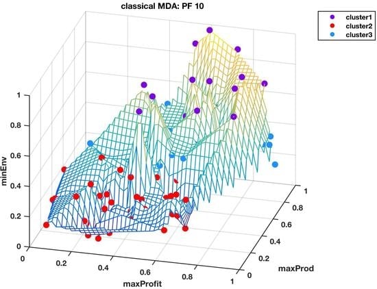
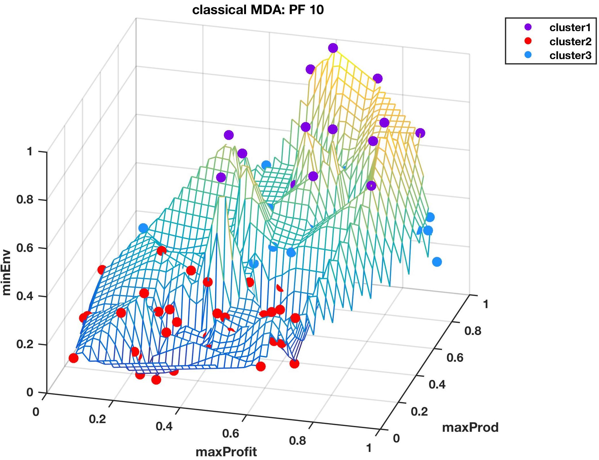
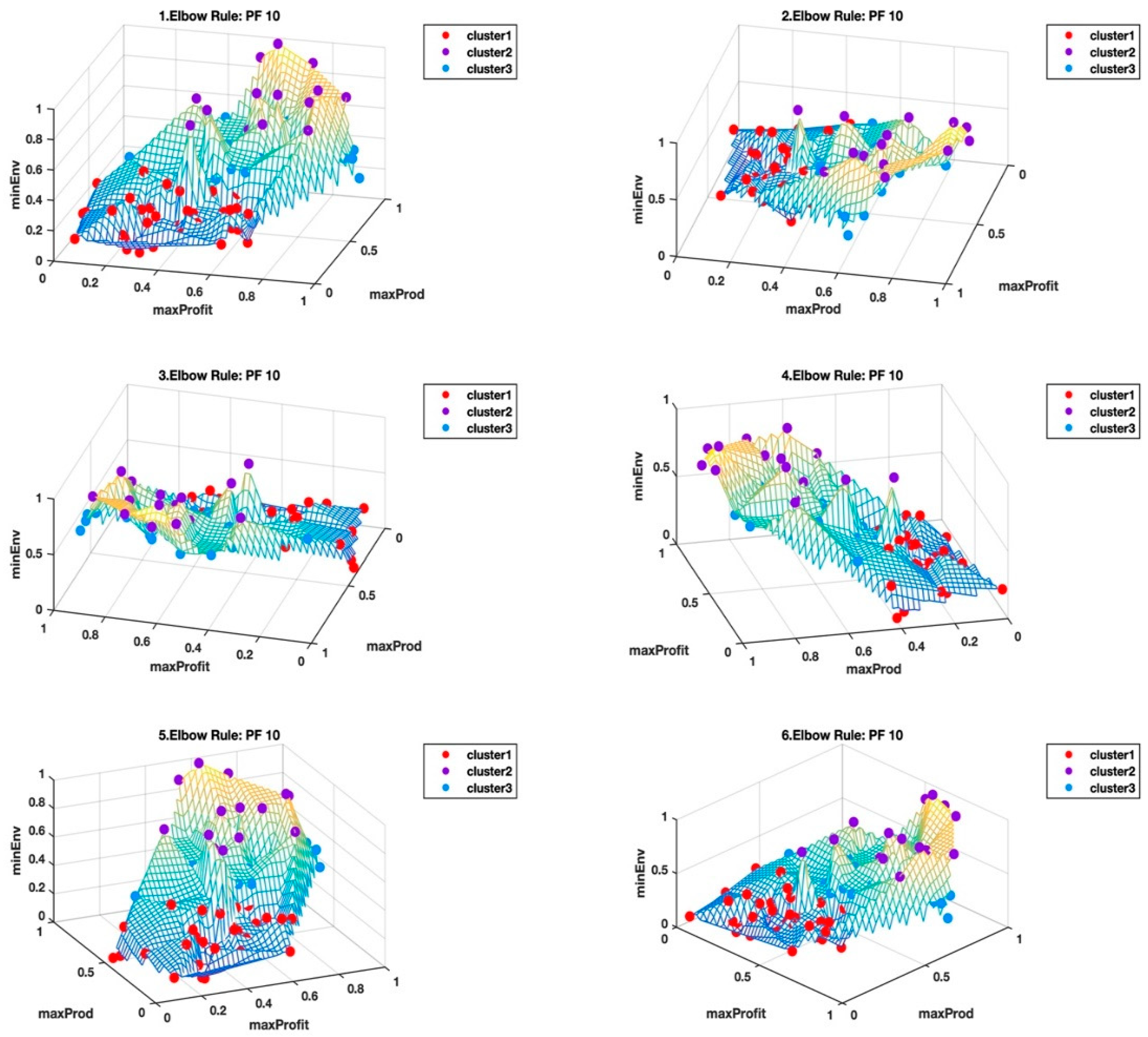
Figure 5 and Figure 6 shows the Pareto front PF10 dataset with six images each in different orientations for a better visual perception of the clustering, based on the highest Calinski–Harabasz criterion method and elbow rule, respectively. The solutions for each cluster are also shown in the captions.
Cluster 1: [1, 2, 4, 7, 8, 9, 10, 11, 13, 14, 15, 16, 17, 20, 22, 24, 27, 29, 31, 32, 34, 36, 37, 41, 44, 46, 47, 49, 51, 56, 57, 59, 60, 62, 63, 65, 66, 68, 69, 70, 71, 72, 73, 74, 76, 77, 79, 80, 81, 83, 84, 85, 86, 88, 91, 92, 93, 94, 95, 97, 98, 99, 100]; and
Cluster 2: [3, 5, 6, 12, 18, 19, 21, 23, 25, 26, 28, 30, 33, 35, 38, 39, 40, 42, 43, 45, 48, 50, 52, 53, 54, 55, 58, 61, 64, 67, 75, 78, 82, 87, 89, 90, 96].
Cluster 1: [3, 5, 6, 12, 15, 33, 35, 38, 39, 40, 42, 43, 48, 54, 55, 57, 58, 59, 61, 64, 66, 67, 79, 87, 89, 90, 96, 99];
Cluster 2: [18, 19, 21, 23, 25, 26, 28, 30, 45, 50, 52, 53, 75, 78, 82]; and
Cluster 3: [1, 2, 4, 7, 8, 9, 10, 11, 13, 14, 16, 17, 20, 22, 24, 27, 29, 31, 32, 34, 36, 37, 41, 44, 46, 47, 49, 51, 56, 60, 62, 63, 65, 68, 69, 70, 71, 72, 73, 74, 76, 77, 80, 81, 83, 84, 85, 86, 88, 91, 92, 93, 94, 95, 97, 98, 100].
From Table 2 and Table 3, we selected the clusters (i.e., CHcluster1 from the Calinski-Harabasz criterion method and ERcluster3 from the elbow rule), with the least average hyper radial distance for Pareto front PF10 dataset. In Figure 5 and Figure 6, CHcluster1 group and ERcluster3 group had many points in common, as they all came from more or less a similar part of the data landscape, i.e., where the environmental impact was low and with moderate profitability and productivity. The total number of solutions in the CHcluster1 group and the ERcluster3 group were 63 and 57, respectively, with a set difference of the following solutions: {15,57,59,66,79,99}. In other words, the set difference defines the set of solutions that was not included in the smaller ERcluster3 group, but included in the larger CHcluster1 group. Another way of getting the same result was to go to the next level up in the average hyper radial distances, i.e., ERcluster1 group from the elbow rule and the CHcluster2 group from the Calinski-Harabasz criterion method. We first find the intersection of the two cluster groups, which we will call cluster n, and then find the set difference between cluster n and ERcluster1 group, which yields the same set: {15,57,59,66,79,99}.
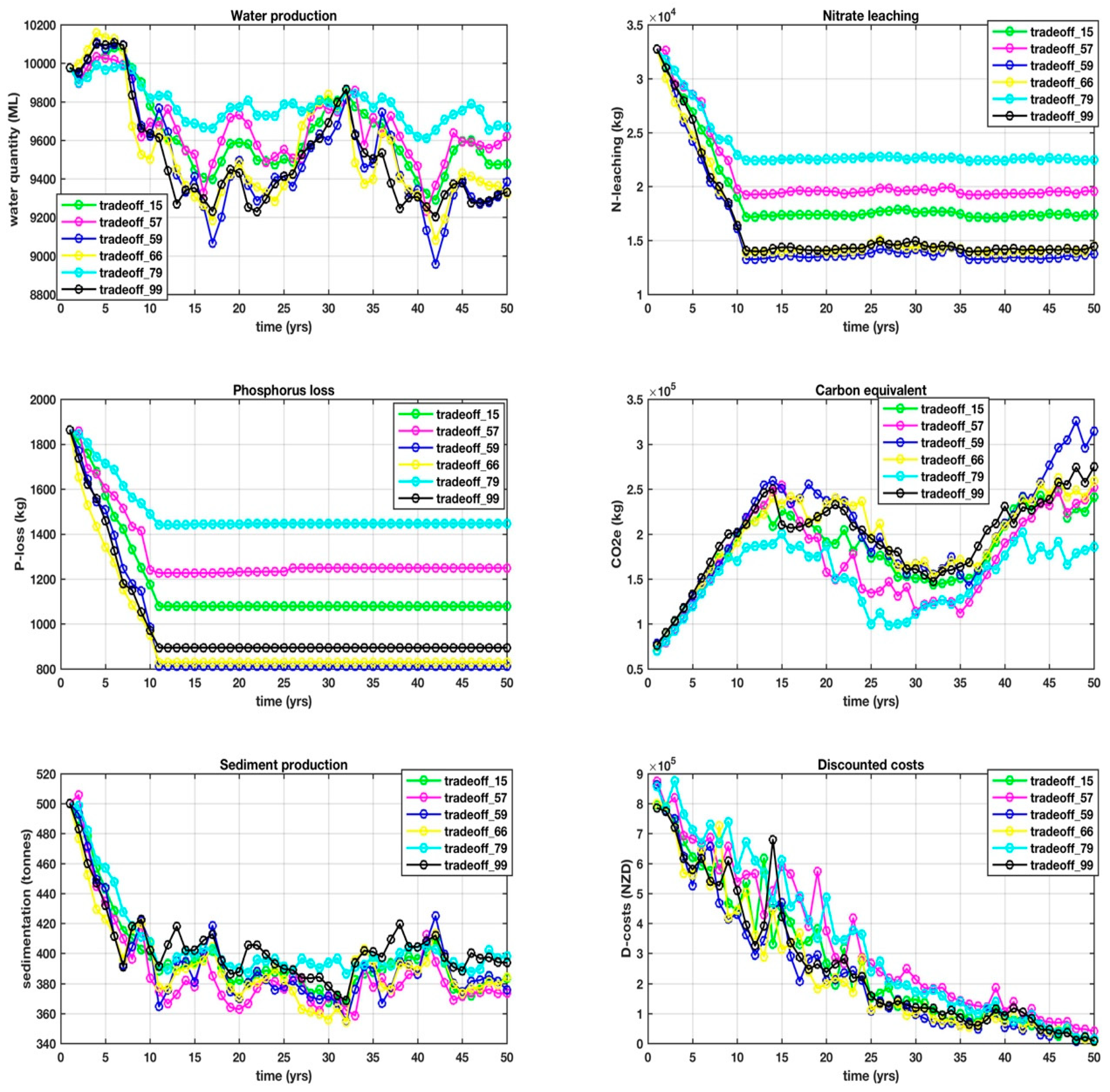
This is where things get interesting, because it is this set difference that defined some of the points that were identified while using other visualization techniques, in particular, DMS that consistently identified 59 and 66. The 14 objectives over a 50 year, one-yearly interval planning horizon for the set difference are shown in Appendix D, with trade-offs between the objectives, making it difficult from which to select a unique solution. Our goal is to arrive at a shortlist of the very best solutions that will form the basis for the next stage of research, which is to identify yet another mathematical process to find the unique solution in near-real-time.
Going back to the set difference list, we are left wondering whether, for the Pareto front datasets, the no-man’s-land region or border may just serve as a way of identifying sweet spots where the short list of the very best solutions resides. We also start to wonder that for difficult datasets with no clear delineation between clusters, the optimal number of clusters might not necessarily be an integer, but may actually be a fractional number. That means for the Pareto front PF10, the optimal number of clusters is between 2 and 3, where the Calinski–Harabasz criterion method finds the minimum of the optimal number of clusters and the elbow rule finds the maximum. Even if this is proven to be the case, the importance might just be the ability of finding the points in the no-man’s-land region, which in this case is verified to carry some of the very best solutions. Out of the set difference list, solutions 57 and 79 were the hardest to find while using the other visual techniques.
When we visualize the points in the no-man’s-land region in Figure 7 and Figure 8, from the highest Calinski–Harabasz criterion method and the elbow rule, respectively, these points look like they form a “fault line” across the middle of the wireframe mesh plot; seemingly, like the two clustering methods have different ways of dealing with these border disputes. As shown in the Table 1 and Table 2 and also the box plots in Figure 3 and Figure 4, it is easy to see the separation of the clusters that is determined by the two clustering methods based on the summary statistics of the hyper radial distances. We can only speculate at this stage that this hyperspace Pareto front has inherent complexity that is not so easy to find, as both the highest Calinski–Harabasz criterion method and the elbow rule have graceful ways of dealing with border disputes. The former method settles the dispute by assigning fewer numbers of clusters and the latter by an increased number of clusters. Only by looking at the clustering results of both methods are we able to realize that there is a border dispute of point belongingness. On the other hand, the interactive visualization, DMS, reveals that the no-man’s-land region is the sweet spot for the shortlist of the very best solutions, which seems to be the balance among the three super objectives, i.e. minimal environmental impact, maximum profitability, and maximum productivity.
We have obviously raised more questions than answers for this exercise and are left with an inconclusive result as to which method would give us an optimal number of clusters for the high dimensional dataset with tightly distributed points. So far, it seems both of the clustering methods are critical and extracting meaning out of the estimated number of clusters from these algorithms, require other information and techniques to make sense of the high-dimensional data. However, we see a way forward by removing subjectivity and bypassing visualization to obtain to a reduced list of the very best solutions. More tests would need to be done to verify the consistency of this procedure that we have presented. In the interim, research to develop the next level of capability that will choose the unique solution in near real-time from the short list will continue.
It is also an interesting observation that is just based on the hyper-radial distance summary statistics, it is inconclusive whether lower profitability and productivity and minimal environmental impact are more preferable than high profitability and productivity, and high environmental impact. Obviously, the data picks the middle ground as the best. This may spark heated debates regarding which extreme is the lesser evil, and we are not inferring anything by it, rather emphasizing the program’s objective choice of middle of the ground, as the data shows.
5. Conclusions
The basis of the suite of tools that were deployed for the unsupervised clustering exercise was the repeatability of results. We found consistency and repeatability of the results in estimating the Calinski–Harabasz criterion while using the agglomerative clustering algorithm that employs the Euclidean distance within clusters and the inner squared distance (i.e., minimum variance) between clusters. With the number of clusters determined, the K-means++ was found to be consistent and efficient in discriminating the clusters for any given number of clusters. The classical MDS from the GEATbx was consistent in the reproducibility of the 3D images.
From such a platform, we were unable to draw the conclusion to which the clustering algorithm between the highest Calinski–Harabasz criterion method and the elbow rule was best in finding the optimal number of clusters, In fact, we are left wondering whether the optimal number of clusters for high dimensional datasets with no clear delineation of clusters is fractional. Note that the datasets that were used for this exercise were not only high-dimensional, but with well-distributed data points from a many-objective optimization, which essentially have no outliers and/or no unique points that stand out. The boundaries of these clusters became a key focus since distance is a key factor in distinguishing separation within and between clusters, where it seems the interesting points of the datasets lay.
We also note that, although there might be merit in basing the optimal number of clusters on either the highest Calinski–Harabasz criterion method, or the elbow rule, caution must be exercised where there are no obvious and distinct clusters in the data. Our take from this is that if one is not sure of the nature of the data under investigation, or it is a mission critical task at hand, then both of the approaches should be used and combined with an innovative way of using extra information, since the optimal number of clusters may be fractional and not an integer.
Author Contributions
Conceptualization, O.C. and V.G.; Methodology, O.C.; Software, O.C. and V.G.; Validation, O.C. and V.G.; Formal analysis, O.C.; Investigation, O.C.; Resources, O.C. and V.G.; Data curation, O.C.; writing—original draft preparation, O.C.; writing—review and editing, O.C.; Visualization, O.C.; Project administration, O.C.
Funding
This research received no external funding.
Acknowledgments
We are grateful to Leonie Chikumbo for assisting with the diagrams and final editing of the document.
Conflicts of Interest
The authors declare no conflict of interest as this piece of research was solely to advance the thinking in clustering algorithm applications, in particular, for difficult multi-dimensional data with no obvious outliers, where the objective is to find a shortlist of “interesting points”.
Appendix A. The Last 10 Pareto Fronts of a Converged Evolutionary Many-Objective Optimization in 3d View
Figure A1.
3D hyperspace Pareto fronts for Pareto fronts 1–5.

The hyperspace Pareto fronts in 3D view look similar but there are differences which may be hard to notice as these are 3D images in 2D viewing. MATLAB gives that extra ability to rotate the images so that the viewer has a much better appreciation of the differences.
Figure A2.
3D hyperspace Pareto fronts for Pareto fronts 6–10.

The wireframe mesh with color change proportional to the Environmental footprint (or height of the 3D plot) makes it that much easier for the viewer to have an appreciation of the location of the points in the in the hyperspace Pareto surface or landscape.
Appendix B. Highest Calinski-Harabasz Criterion-Based Clustering in 3D View
Figure A3.
Cluster identification based on the highest Calinski-Harabasz criterion for Pareto fronts, PF1–PF5.
Figure A3.
Cluster identification based on the highest Calinski-Harabasz criterion for Pareto fronts, PF1–PF5.

The “optimal” number of clusters based on the highest Calinski-Harabasz criterion was consistently two for all the hyperspace Pareto fronts. Each color connotes a different cluster. This may seem to make sense as there is a cluster depicting the highs and another depicting the valleys. However, note that CHarabasz: PF4 is difficult to understand as the generality of highs and valleys seem to break down here. A quick comparison with the elbow rule equivalence in Appendix C (Elbow Rule: PF4) shows a much better discrimination with three clusters.
Figure A4.
Cluster identification based on the highest Calinski-Harabasz criterion for Pareto fronts PF6–PF10.
Figure A4.
Cluster identification based on the highest Calinski-Harabasz criterion for Pareto fronts PF6–PF10.

For these last five hyperspace Pareto fronts, one could not fault the classification of these surfaces into two clusters, seemingly fitting the generalization of the highs and the lows/valleys. The above visualizations look convincingly so.
Appendix C. The Elbow Rule-Based Clustering in 3D View
Figure A5.
Cluster identification based on the elbow rule for Pareto fronts, PF1–PF5.

The elbow rule reveals three clusters in the above hype Pareto fronts, which were not so obvious, but the above visualizations makes a convincing case. All of a sudden two clusters (as determined from just selecting the number of clusters associated with the highest Calinski-Harabasz criterion) seem like just a generalization for these kinds of multi-dimensional datasets.
Figure A6.
Cluster identification based on the elbow rule for Pareto fronts, PF6–PF10.

Although the elbow rule generally identified three clusters for the hyperspace Pareto fronts, four clusters were identified in Elbow Rule: PF9. From the visualization it is easy to perceive the gradual progression from the lows to the highs.
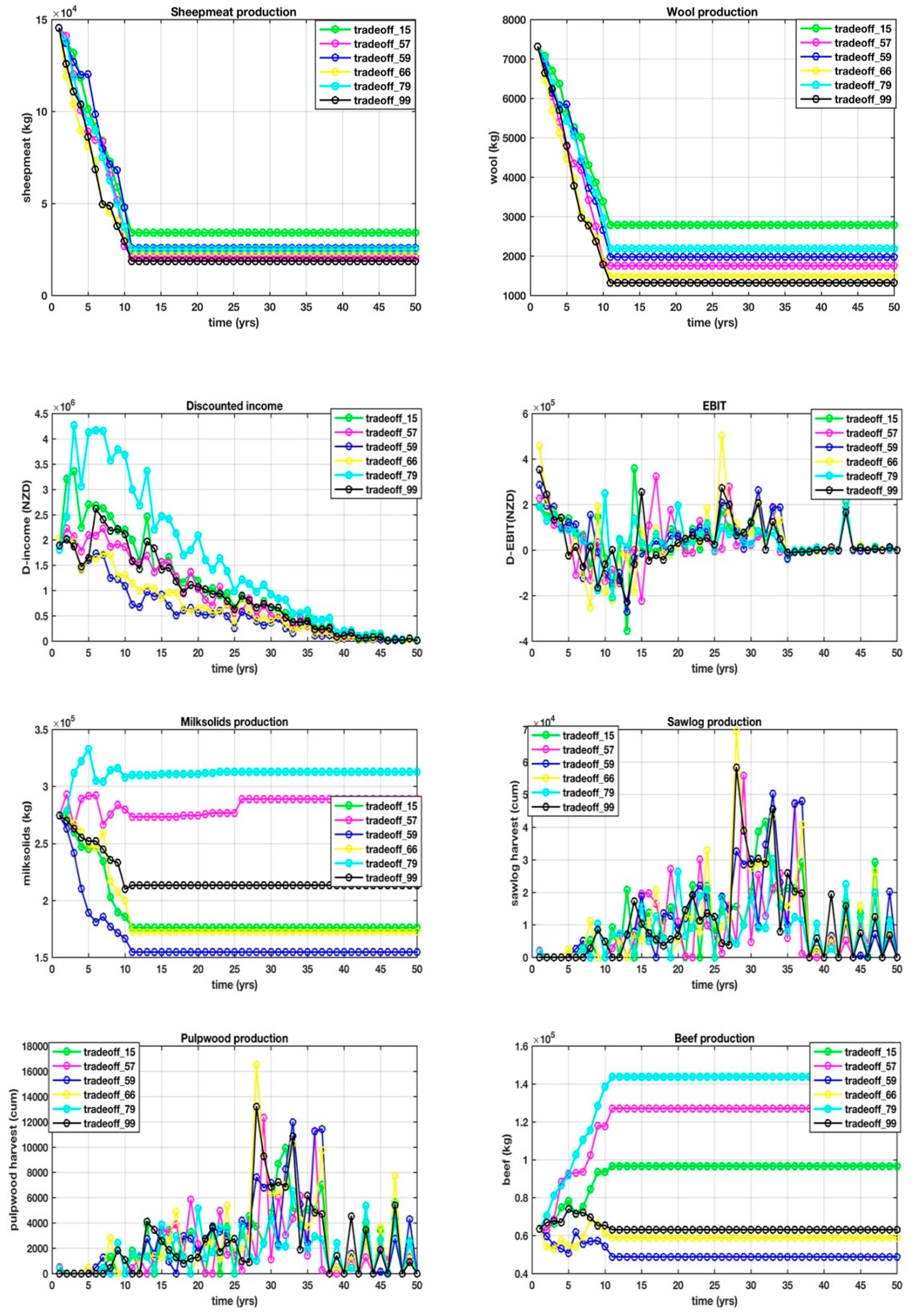
Appendix D. The 14 Objectives from the Pareto Front PF10 Shown over the 50-year Planning Period at one yearly Time Interval. The Solutions Shown Are from the Shortlist, {15, 57, 59, 66, 79, 99}
Figure A7.
Time-series objectives over the 50-year time horizon for solutions, 15, 57, 59, 66, 79, and 99, for water production, nitrate leaching, phosphorus loss, carbon equivalent, sediment production and discounted costs.
Figure A7.
Time-series objectives over the 50-year time horizon for solutions, 15, 57, 59, 66, 79, and 99, for water production, nitrate leaching, phosphorus loss, carbon equivalent, sediment production and discounted costs.

Figure A8.
Time-series objectives over the 50-year time horizon for solutions, 15, 57, 59, 66, 79, and 99, for sheepmeat production, wool production, discounted income, EBIT, milksolids production, salog production, pulpwood production and beef production.
Figure A8.
Time-series objectives over the 50-year time horizon for solutions, 15, 57, 59, 66, 79, and 99, for sheepmeat production, wool production, discounted income, EBIT, milksolids production, salog production, pulpwood production and beef production.

References
- Keim, D.A.; Panse, C.; Schneidewind, J.; Sips, M.; Hao, M.C.; Dayal, U. Pushing the limit in Visual Data Exploration: Techniques and Applications. In KI 2003: Advances in Artificial Intelligence, Lecture Notes in Computer Science; Springer: Berlin, Germany, 2003; Volume 2821, pp. 37–51. [Google Scholar]
- Hund, M.; Böhm, D.; Sturm, W.; Sedlmair, M.; Schreck, T.; Ullrich, T.; Keim, D.A.; Majnaric, L.; Holzinger, A. Visual analytics for concept exploration in subspaces of patient groups. Brain Inform. 2016, 3, 233–247. [Google Scholar] [PubMed]
- Henderson, P. Sammon mapping. Pattern Recognit. Lett. 1997, 18, 1307–1316. [Google Scholar]
- Wegman, E.J.; Solka, J.L. On some mathematics for visualizing high dimensional data. Indian J. Stat. 2001, 64, 429–452. [Google Scholar]
- Wickham, H.; Cook, D.; Hofmann, H.; Buja, A. Tourr: An R package for exploring multivariate data with projections. J. Stat. Softw. 2011, 40, 1–18. [Google Scholar] [CrossRef]
- Wegman, E.J. Visualization Methods for the Exploration of High Dimensional Data, US Army Research Office Rpt DAAL03-91-G-0039; George Mason University, Centre for Computational Statistics: Fairfax, VA, USA, 1995; 5p. [Google Scholar]
- Wegman, E.J.; Carr, D.B. Statistical graphics and visualization. In Computational Statistics; Rao, C.R., Ed.; Handbook of Statistics: North-Holland, Amsterdam, 1993; Volume 9, pp. 857–958. [Google Scholar]
- Savoska, S.; Loskovska, S. Parallel coordinates as a tool of exploratory data analysis. In Proceedings of the 17th Telecommunications forum, TELFOR 2009, Serbia, Belgrade, 24–26 November 2009; pp. 1343–1346. [Google Scholar]
- Inselberg, A. The plane with parallel coordinates. Visual Comput. 1985, 1, 69–91. [Google Scholar]
- Fienberg, S. Graphical methods in statistics. Am. Stat. 1979, 33, 165–178. [Google Scholar]
- Kohonen, T. Self-Organized Formation of Topologically Correct Feature Maps. Biol. Cybern. 1982, 43, 59–69. [Google Scholar] [CrossRef]
- Bro, R.; Smilde, A.K. Principal component analysis. R. Soc. Chem. Anal. Methods 2014, 6, 2812–2831. [Google Scholar]
- Granville, V. Applied Stochastic Processes, Chaos Modeling and Probabilistic Properties of Numeration Systems; Data Science Central: Seattle, WA, USA, 2018; 104p. [Google Scholar]
- Arthur, D.; Vassilvitskii, S. K-means++: The advantages of careful seeding. In Proceedings of the 18th Annual ACM-SIAM Symposium on Discrete Algorithms, New Orleans, LA, USA, 7–9 January 2007; pp. 1027–1035. [Google Scholar]
- Sammon, J.W., Jr. A nonlinear mapping for data structure analysis. IEEE Trans. Comput. 1969, C-18, 401–409. [Google Scholar]
- Chikumbo, O.; Mitchell, H.; Vallance, R. Determining profitability for Ngati Whakaue Tribal Lands Inc., farms by developing a sustainable land management plan. N. Z. J. For. Sci. 2011, 41, 3–40. [Google Scholar]
- Whitehead, I.D. STANDPAK stand modelling system for radiata pine. In New Approaches to Spacing and Thinning in Plantation Forestry; James, R.N., Tarlton, G.L., Eds.; FRI Bulletin No 151; Ministry of Forestry: Wellington, New Zealand, 1990. [Google Scholar]
- Beets, P.N.; Robertson, K.A.; Ford-Robertson, J.B.; Gordon, J.; Maclaren, J.P. Description and validation of C change: A model for simulating carbon content in managed Pinus radiata stands. N. Z. J. For. Sci. 1999, 29, 409–427. [Google Scholar]
- Warner, M. Putting the Sustainable ‘Development’ Performance of Companies on the Balance Sheet; Overseas Development Institute: London UK, 2003. [Google Scholar]
- Bryant, J.R.; Ogle, G.; Marshall, P.R.; Glassey, C.B.; Lancaster, J.A.S.; García, S.C.; Holmes, C.W. Description and evaluation of the Farmax Dairy Pro decision support model. N. Z. J. Agric. Res. 2010, 53, 13–28. [Google Scholar] [CrossRef] [Green Version]
- de Castro, L.N. Fundamentals of natural computing: An overview. Phys. Life Rev. 2007, 4, 1–36. [Google Scholar] [CrossRef]
- Godefroid, P.; Khurshid, S. Exploring the very large state spaces using genetic algorithms. In Proceedings of the 8th International Conference on Tools and Algorithms for the construction and Analysis of Systems, Grenoble, France, 8–12 April 2002; Katoen, J.-P., Stevens, P., Eds.; Springer: Berlin/Heiderberg, Germany, 2002; pp. 266–280. [Google Scholar]
- Holland, J.H. Genetic Algorithms. 1986. Available online: https://wiki.eecs.yorku.ca/course_archive/2011-12/F/4403/_media/genetic_algorithms.pdf (accessed on 3 September 2017).
- Blumenfeld, O.O.; Patnaik, S.K. Allelic genes of blood group antigens: A source of human mutations and cSNPs documented in the Blood Group Antigen Gene Mutation Database. Hum. Mutat. 2004, 23, 8–16. [Google Scholar] [CrossRef] [PubMed]
- Cheung, J.C.; Deber, C.M. Misfolding of the cystic fibrosis transmembrane conductance regulator and disease. Biochemistry 2008, 47, 1465–1473. [Google Scholar] [CrossRef]
- Chikumbo, O.; Goodman, E.; Deb, K. The triple bottomline many-objective-based decision making for a land use management problem. J. Multi-Criteria Decis. Anal. 2015, 22, 133–159. [Google Scholar] [CrossRef]
- Kruskal, J.B. Multidimensional scaling by optimizing goodness of fit to a non-metric hypothesis. Psychometrika 1964, 29, 1–27. [Google Scholar] [CrossRef]
- Lerner, B.; Guterman, H.; Aladjem, M.; Dinstein, I. On the initialization of Sammon’s nonlinear mapping. Patterns Anal. Appl. 2000, 3, 61–68. [Google Scholar] [CrossRef]
- Ripley, B.D. Pattern Recognition and Neural Networks; Cambridge University Press: Cambridge, UK, 1996; Chapter 9. [Google Scholar]
- Pohlheim, H. GEATbx: Introduction, Evolutionary Algorithms: Overview, Methods and Operators. 2006. Available online: www.geatbx.com (accessed on 4 June 2019).
- MathWorks Inc. Statistics and Machine Learning Toolbox; Package: Clustering.evaluation, Documentation; MathWorks Inc.: Natick, MA, USA, 2015. [Google Scholar]
- Bishop, C.M. Pattern Recognition and Machine Learning; Springer: Berlin, Germany, 2006; 738p. [Google Scholar]
- Sahbi, H. A particular Gaussian mixture model for clustering and its application to image retrieval. Soft Comput. 2008, 12, 667–676. [Google Scholar] [CrossRef]
- Thorndike, R.L. Who belongs in the family? Psychometrika 1953, 18, 267–276. [Google Scholar] [CrossRef]
- Granville, V. How to Automatically Determine the Number of Clusters in Your Data—And More. 2019. Available online: https://www.datasciencecentral.com/profiles/blogs/how-to-automatically-determine-the-number-of-clusters-in-your-dat (accessed on 4 June 2019).
- Lloyd, S.P. Least squares quantization in PCM. IEEE Trans. Inform. Theory 1982, 28, 129–137. [Google Scholar] [CrossRef]
- Chiu, P.-W.; Naim, A.M.; Bloebaum, C.L. The hyper-radial visualization method for multi-attribute decision-making under certainty. Int. J. Prod. Dev. 2009, 9, 4–31. [Google Scholar] [CrossRef]
- Naim, A.M.; Chiu, P.-W.; Bloebaum, C.L.; Lewis, K.E. Hyper-radial visualization for multi-objective decision-making support under uncertainty using preference ranges: The PRUF method. In Proceedings of the 12th AIAA/ISSMO Multidisciplinary Analysis and Optimization Conference, Victoria, BC, Canada, 10–12 September 2009. [Google Scholar]
- Balling, R. Design by shopping: A new paradigm? In Proceedings of the 3rd World Congress of Structural and Multidisciplinary Optimization (WCSMO-3), University at Buffalo, Buffalo, NY, USA, 17–21 May 1999; pp. 295–297. [Google Scholar]
Figure 1.
The heterogenous data used to formulate the many-objective optimization problem with 14 objectives ranging from water quantity to wool production.
Figure 1.
The heterogenous data used to formulate the many-objective optimization problem with 14 objectives ranging from water quantity to wool production.

Figure 2.
A visualization comparison between outputs from classical Multi-Dimensional Scaling (on the left) and Sammon’s nonlinear mapping (on the right) for the 100th generation Pareto front with clusters estimated using the elbow rule.
Figure 2.
A visualization comparison between outputs from classical Multi-Dimensional Scaling (on the left) and Sammon’s nonlinear mapping (on the right) for the 100th generation Pareto front with clusters estimated using the elbow rule.

Figure 3.
Box plots for the cluster medians and the 25th and 75th percentiles. This is shown for the hyper-radial distance estimates from both the highest Calinski–Harabasz criterion (i.e., CHcluster#) and the elbow rule (i.e., ERcluster#) of Pareto fronts 1–5.
Figure 3.
Box plots for the cluster medians and the 25th and 75th percentiles. This is shown for the hyper-radial distance estimates from both the highest Calinski–Harabasz criterion (i.e., CHcluster#) and the elbow rule (i.e., ERcluster#) of Pareto fronts 1–5.

Figure 4.
Box plots for the cluster medians and the 25th and 75th percentiles. This is shown for the hyper-radial distance estimates from both the highest Calinski–Harabasz criterion (i.e., CHcluster#) and the elbow rule (i.e., ERcluster#) of Pareto fronts 6–10.
Figure 4.
Box plots for the cluster medians and the 25th and 75th percentiles. This is shown for the hyper-radial distance estimates from both the highest Calinski–Harabasz criterion (i.e., CHcluster#) and the elbow rule (i.e., ERcluster#) of Pareto fronts 6–10.

Figure 5.
Sammon’s nonlinear mapping three-dimensional (3D) projections for Pareto Front 10 based on the number of clusters derived from the highest Calinski-Harabasz criterion. Six images are shown in different views that are rotated from 1–6 in a clockwise direction. The two clusters include the following solutions:

Figure 6.
Sammon’s nonlinear mapping 3D projections for Pareto Front 10 based on the number of clusters derived from the elbow rule. Six images are shown in different views that are rotated from 1–6 in a clockwise direction. The three clusters include the following solutions:
Figure 6.
Sammon’s nonlinear mapping 3D projections for Pareto Front 10 based on the number of clusters derived from the elbow rule. Six images are shown in different views that are rotated from 1–6 in a clockwise direction. The three clusters include the following solutions:

Figure 7.
Highest Calinski–Harabasz criterion method clustering with the no-man’s-land points superimposed in yellow in the CHcluster1 group.
Figure 7.
Highest Calinski–Harabasz criterion method clustering with the no-man’s-land points superimposed in yellow in the CHcluster1 group.

Figure 8.
Elbow rule clustering with the no-man’s-land points superimposed in yellow in the ERcluster3 group.
Figure 8.
Elbow rule clustering with the no-man’s-land points superimposed in yellow in the ERcluster3 group.


Table 1.
Optimal/near optimal number of clusters for 10, 14-dimensional Pareto fronts predicted from the highest Calinski–Harabasz criterion and the elbow rule.
Table 1.
Optimal/near optimal number of clusters for 10, 14-dimensional Pareto fronts predicted from the highest Calinski–Harabasz criterion and the elbow rule.
| Pareto front | 1 | 2 | 3 | 4 | 5 | 6 | 7 | 8 | 9 | 10 |
| Highest Calinski–Harabasz criterion estimated no. of clusters | 2 | 2 | 2 | 2 | 2 | 2 | 2 | 2 | 2 | 2 |
| Elbow rule estimated no. of clusters | 3 | 3 | 3 | 3 | 3 | 3 | 3 | 3 | 4 | 3 |
Table 2.
Highest Calinski–Harabasz criterion-based cluster means and standard deviations for hyper-radial distances of Pareto Fronts, 1–10.
Table 2.
Highest Calinski–Harabasz criterion-based cluster means and standard deviations for hyper-radial distances of Pareto Fronts, 1–10.
| Pareto Front | Cluster 1 Mean | Cluster 1 std Deviation | Cluster 2 Mean | Cluster 2 std Deviation |
|---|---|---|---|---|
| PF1 | 0.3324 | 0.1391 | 0.7613 | 0.1295 |
| PF2 | 0.7728 | 0.1242 | 0.3133 | 0.1322 |
| PF3 | 0.7717 | 0.1244 | 0.3138 | 0.1368 |
| PF4 | 0.5208 | 0.2744 | 0.4959 | 0.2974 |
| PF5 | 0.3063 | 0.1274 | 0.7750 | 0.1149 |
| PF6 | 0.7607 | 0.1259 | 0.3302 | 0.1373 |
| PF7 | 0.3114 | 0.1321 | 0.7556 | 0.1338 |
| PF8 | 0.3134 | 0.1304 | 0.7621 | 0.1283 |
| PF9 | 0.2848 | 0.1390 | 0.7981 | 0.1403 |
| PF10 | 0.3138 | 0.1368 | 0.7717 | 0.1244 |
Table 3.
The means for the elbow rule-based optimal clustering and standard deviations for hyper-radial distances of Pareto Fronts, 1–10.
Table 3.
The means for the elbow rule-based optimal clustering and standard deviations for hyper-radial distances of Pareto Fronts, 1–10.
| Pareto Front | Cluster 1 Mean | Cluster 1 std Deviation | Cluster 2 Mean | Cluster 2 std Deviation | Cluster 3 Mean | Cluster 3 std Deviation | Cluster 4 Mean | Cluster 4 std Deviation |
|---|---|---|---|---|---|---|---|---|
| PF1 | 0.6664 | 0.1133 | 0.8471 | 0.1129 | 0.3032 | 0.1204 | ||
| PF2 | 0.6779 | 0.1136 | 0.8294 | 0.1255 | 0.2941 | 0.1187 | ||
| PF3 | 0.8572 | 0.1168 | 0.2916 | 0.1236 | 0.6729 | 0.1155 | ||
| PF4 | 0.9095 | 0.0900 | 0.2728 | 0.1208 | 0.6765 | 0.1153 | ||
| PF5 | 0.2897 | 0.1149 | 0.7005 | 0.1055 | 0.8499 | 0.1158 | ||
| PF6 | 0.8423 | 0.1193 | 0.2993 | 0.1194 | 0.6624 | 0.1169 | ||
| PF7 | 0.6110 | 0.1389 | 0.8240 | 0.1316 | 0.2727 | 0.1126 | ||
| PF8 | 0.2874 | 0.1164 | 0.8895 | 0.1072 | 0.6549 | 0.1246 | ||
| PF9 | 0.9903 | 0.0120 | 0.6357 | 0.1326 | 0.8280 | 0.1009 | 0.2494 | 0.1171 |
| PF10 | 0.6729 | 0.1155 | 0.8572 | 0.1168 | 0.2916 | 0.1236 |
© 2019 by the authors. Licensee MDPI, Basel, Switzerland. This article is an open access article distributed under the terms and conditions of the Creative Commons Attribution (CC BY) license (http://creativecommons.org/licenses/by/4.0/).
Share and Cite
MDPI and ACS Style
Chikumbo, O.; Granville, V. Optimal Clustering and Cluster Identity in Understanding High-Dimensional Data Spaces with Tightly Distributed Points. Mach. Learn. Knowl. Extr. 2019, 1, 715-744. https://doi.org/10.3390/make1020042
AMA Style
Chikumbo O, Granville V. Optimal Clustering and Cluster Identity in Understanding High-Dimensional Data Spaces with Tightly Distributed Points. Machine Learning and Knowledge Extraction. 2019; 1(2):715-744. https://doi.org/10.3390/make1020042
Chicago/Turabian StyleChikumbo, Oliver, and Vincent Granville. 2019. "Optimal Clustering and Cluster Identity in Understanding High-Dimensional Data Spaces with Tightly Distributed Points" Machine Learning and Knowledge Extraction 1, no. 2: 715-744. https://doi.org/10.3390/make1020042