Generalization of Parameter Selection of SVM and LS-SVM for Regression

Abstract

A Support Vector Machine (SVM) for regression is a popular machine learning model that aims to solve nonlinear function approximation problems wherein explicit model equations are difficult to formulate. The performance of an SVM depends largely on the selection of its parameters. Choosing between an SVM that solves an optimization problem with inequality constrains and one that solves the least square of errors (LS-SVM) adds to the complexity. Various methods have been proposed for tuning parameters, but no article puts the SVM and LS-SVM side by side to discuss the issue using a large dataset from the real world, which could be problematic for existing parameter tuning methods. We investigated both the SVM and LS-SVM with an artificial dataset and a dataset of more than 200,000 points used for the reconstruction of the global surface ocean CO₂ concentration. The results reveal that: (1) the two models are most sensitive to the parameter of the kernel function, which lies in a narrow range for scaled input data; (2) the optimal values of other parameters do not change much for different datasets; and (3) the LS-SVM performs better than the SVM in general. The LS-SVM is recommended, as it has less parameters to be tuned and yields a smaller bias. Nevertheless, the SVM has advantages of consuming less computer resources and taking less time to train. The results suggest initial parameter guesses for using the models.

1. Introduction

Machine intelligence has emerged as an important player in transforming everything from daily life to scientific research [1]. In the broad spectrum of machine learning models, Support Vector Machine (SVM) is one of the most widely used models. In geosciences, SVMs have been used to interpolate scarce measurements to regional [2,3,4], continental [5,6] and global scales [7,8]. SVM was introduced in the early 1990s [9] for classification and later extended to function regression [10]. As the SVM for regression includes inequality constrains, its results could be biased in comparison with the target. The Least Square Support Vector Machine (LS-SVM) for regression [11] is a reformulated SVM that minimizes the square error between the model and the target. The equality constrains significantly reduce the possibility of making a biased prediction.

It is well known that the performance of an SVM depends strongly on the selection of its parameters. Exhaustive grid search and a cross-validation method [5,6,12] were traditionally employed to obtain optimal parameter values. With a large dataset, parameter tuning could become too expensive to be practical for an office PC due to long computing time and lack of prior knowledge of the parameters. Several alternative methods have been proposed to speed up the search [13,14,15,16,17,18,19,20]. However, they were tested either with only toy examples or with real world data of a few hundreds to a few thousands of samples. Unless a software includes parameter tuning tools, implementing methods is not a simple task for many users. Meanwhile, an automatic tuning tool, for example the MATLAB toolbox of [11,21], may not work with a large dataset or may take a very long time to compute.

We investigated both the SVM and LS-SVM with an artificial dataset and a dataset used for the global surface ocean CO₂ mapping, which included more than 200,000 data points. The results would give users general hints for picking up initial parameter guesses and tuning parameters effectively. The side-by-side comparison would also help users to understand the differences between the two models.

2. Materials and Methods

2.1. Models

Given a training dataset {x_i, y_i} with x_i ∈ ℜ^p being an input, y_i ∈ ℜ¹ being the target output, and i∈(1,n), the goal of the SVM for regression is to find a function that has at most ε deviation from y_i for all the training data and at the same time is as flat as possible [10], i.e.,

$$f\left({\mathit{x}}_{\mathit{i}}\right)={\mathit{w}}^T\mathit{\phi }\left({\mathit{x}}_{\mathit{i}}\right)+b.$$

(1)

where w, φ(x_i) ∈ ℜⁿ and b is a constant. The function φ(x_i) maps the p-dimensional space of x_i to a much higher dimensional space, resulting in a generalized model that can be used to solve various nonlinear problems without having to know the explicit relation between the target and the inputs.

The flatness condition can be formulated to the convex optimization problem:

$$\begin{array}{l}\mathrm{minimize}\frac{1}{2}{\mathit{w}}^{\mathrm{T}}\mathit{w}\\ \mathrm{subject}\mathrm{to}\{\begin{array}{c}{\mathit{w}}^T\mathit{\phi }\left({\mathit{x}}_{\mathit{i}}\right)+b-y_{\mathrm{i}}\le \epsilon \\ y_{\mathrm{i}}-{\mathit{w}}^{\mathrm{T}}\mathit{\phi }\left({\mathit{x}}_{\mathrm{i}}\right)-b\le \epsilon \end{array}.\end{array}$$

(2)

The inequity constrains indicate that data points having errors smaller than ε are ignored or not counted as support vectors. As there may not be a function that approximates all (x_i, y_i) pairs with ε precision, a pair of slack variables were introduced to cope with the infeasible constraints. The optimization problem becomes:

$$\begin{array}{l}\mathrm{minimize}\frac{1}{2}{\mathit{w}}^T\mathit{w}+C{\displaystyle {\displaystyle \sum }_{i=1}^n}\left({\xi }_i+{\xi }_i^{*}\right),C>0,\\ \mathrm{subject}\mathrm{to}\{\begin{array}{l}{\mathit{w}}^T\mathit{\phi }\left({\mathit{x}}_{\mathit{i}}\right)+b-y_i\le \epsilon +{\xi }_i^{*}\\ y_i-{\mathit{w}}^T\mathit{\phi }\left({\mathit{x}}_{\mathit{i}}\right)-b\le \epsilon +{\xi }_i\end{array}and{\xi }_i,{\xi }_i^{*}\ge 0.\end{array}$$

(3)

The parameter C determines the trade-off between the flatness of the function and the amount up to which deviations larger than ε are tolerated. Applying Lagrange multipliers to the problem above yields a dual optimization problem:

$$\begin{array}{l}\mathrm{minimize}\{\begin{array}{l}\frac{1}{2}{\left(\mathit{\alpha }-{\mathit{\alpha }}^{*}\right)}^T\Omega \left(\alpha -{\alpha }^{*}\right)\\ \epsilon {\displaystyle {\displaystyle \sum }_{i=1}^n}\left({\alpha }_i-{\alpha }_i^{*}\right)-{\displaystyle {\displaystyle \sum }_{i=1}^n}{y}_i\left({\alpha }_i-{\alpha }_i^{*}\right)\end{array}\\ \mathrm{subject}\mathrm{to}{\displaystyle {\displaystyle \sum }_{i=1}^n}\left({\alpha }_i-{\alpha }_i^{*}\right)=0and0\le {\alpha }_i,{\alpha }_i^{*}\le C,\end{array}$$

(4)

where α_i are coefficients to be solved and Ω is a n by n matrix with

$${\mathsf{\Omega }}_{ij}=K\left({\mathit{x}}_{\mathit{i}},{\mathit{x}}_j\right)=\mathit{\phi }{\left({\mathit{x}}_{\mathit{i}}\right)}^T\mathit{\phi }\left({\mathit{x}}_j\right).$$

(5)

The kernel function K(x_i,x_j) may take several forms. Our investigation focused on the most used radical basis function:

$$K\left({\mathit{x}}_i,{\mathit{x}}_j\right)=\exp \left(-\frac{{\Vert {\mathit{x}}_i-{\mathit{x}}_j\Vert }^2}{2{\sigma }^2}\right),$$

(6)

where σ is a parameter affecting the shape of the hyperplane of the SVM. After solving Equation (4), the approximate function (1) becomes:

$$f\left({\mathit{x}}_i\right)={\sum }_{j=1}^n\left({\alpha }_i-{\alpha }_i^{*}\right)K\left({\mathit{x}}_i,{\mathit{x}}_j\right)+b.$$

(7)

Instead of the inequality constrains, the LS-SVM algorithm [11] reformulates Equation (2) with a least square error function, i.e.,

$$\begin{array}{l}\mathrm{minimize}\frac{1}{2}\left({\mathit{w}}^T\mathit{w}+\gamma {\mathit{e}}^T\mathit{e}\right),\\ \mathrm{subject}\mathrm{to}{e}_i=y_i-{\mathit{w}}^T\mathit{\phi }\left({\mathit{x}}_i\right)-b.\end{array}$$

(8)

where γ > 0 is the tradeoff parameter for function approximation error. Solving the problem by the Lagrange multipliers eventually yields:

$$\left[\begin{array}{cc}0& {\mathit{u}}^T\\ \mathit{u}& \Omega +{\gamma }^{-1}\mathit{I}\end{array}\right]\left[\begin{array}{c}b\\ \mathit{\alpha }\end{array}\right]=\left[\begin{array}{c}0\\ \mathit{y}\end{array}\right],$$

(9)

where u is a n × 1 vector with all entries being 1. After solving Equation (9), the approximate function (1) becomes:

$$f\left({\mathit{x}}_i\right)={\displaystyle \sum }_{j=1}^n{\alpha }_{i}K\left({\mathit{x}}_i,{\mathit{x}}_j\right)+b.$$

(10)

In summary, the parameters to be optimized include the ε and C in Equation (4) for the SVM, the γ in Equation (9) for the LS-SVM, and the σ in Equation (6) for both the SVM and LS-SVM. It is not difficult to see that the larger the σ, the flatter the hyperplane and therefore the less capable the kernel is to fit a nonlinear function. Because of the different constrains, a distinguished difference between the SVM and LS-SVM is that all the training data points are included as the support vectors of the LS-SVM, whereas the SVM excludes those points whose distance from the hyperplane is less than ε. The C parameters also affects the number of support vectors of the SVM through the soft margin. Regarding the LS-SVM, the inverse of the γ is equivalent to the regularization factor for solving the ill-conditioned linear system equations. A smaller γ indicates more precise fitting of a function.

2.2. Software

We used the standalone freeware LibSVM [22] for the SVM model. Although there are other freeware like SVMLight [23] and SVMTorch [24], they had problems with large datasets in our test. For the LS-SVM, there was no standalone freeware to our knowledge. Available MATLAB toolboxes, such as LS-SVMlab [11] and StatLSSVM [21], had problems with our large CO₂ dataset. We have written a standalone freeware available at http://united-csfe.com/fcew/ann.zip. It implements a conjugate-gradient method to solve a large linear equation efficiently and includes the option to normalize data internally to release users from the normalization procedure.

2.3. Data

The first dataset includes 1000 generated random data in (−1,1) for five input variables. The target was calculated by:

$$y=x_1\cos \left(x_2\right)+\frac{x_3\exp \left(x_4\right)}{1+0.9x_5}.$$

(11)

The dataset was used mainly to demonstrate the behavior of the SVM and LS-SVM in two extreme settings. The first setting simulates a perfect nonlinear dependence of y on five independent variables, i.e., the target includes no noise; the second setting uses one of the five x variables as the target and other four as inputs to simulate the extreme case that the target are all noises. The data were split into two equal parts, one for training and the other for validation.

The second dataset is an update of the one used for the reconstruction of the global surface ocean CO₂ concentration [25], which was assumed to be the function of latitude (LAT), sea surface temperature (SST), sea surface salinity (SSS), surface chlorophyll concentration (CHL), mixed layer depth (MLD), and month (MON), i.e.,

$${\mathrm{CO}}_2=f\left(\mathrm{LAT},\mathrm{SST},\mathrm{SSS},\mathrm{CHL},\mathrm{MLD},\mathrm{CMON},\mathrm{SMON}\right),$$

(12)

where CMON and SMON are the cosine and sine transform of MON, respectively.

The CO₂ data came from the SOCAT version 6.0 product [26]. A total of 207,393 data points was extracted for the 1990-2017 period using the criteria set by [8]. The linear trend of CO₂ was estimated by the method of [8] and the CO₂ data were adjusted to the reference year of 2005. The monthly means of SST were extracted from the Optimum Interpolation V2 product [27], SSS from the World Ocean Atlas 2013 product [28], CHL from the SNPP VIIRS climatology of NASA [29], and MLD from the Monthly Isopycnal and Mixed-layer Ocean Climatology [30]. Z-normalization was applied to the input variables, i.e.,

$$x_i^{\prime }=\frac{x_i-\overline{x_i}}{{\sigma }_i}.$$

(13)

Many studies on parameter optimization used raw data. In extreme cases, the outcome of the kernel function could be dominated by certain variables that vary in a large range; therefore, scaling data of independent variables to remove units is important to generalize the results of parameter optimization.

We did not scale the target variable for the convenience of checking the output directly. One must be aware that the optimal ε of the SVM is expected to be on a similar scale as the standard deviation of the target in most cases.

Ten CO₂ datasets were derived from the primary dataset for Monte Carlo cross-validation [31]. Each derived dataset comprises of 10% of randomly sampled data from the primary data for training and the remaining 90% for validation. A different random seed was used for each random sampling. There are two reasons for choosing the sample ratio of training and validation. First, the matrix size for solving Equation (9) is the square of the sample size. If a large proportion of the primary data was used for training, the matrix alone would exhaust the memory of a PC or training would take too long to be practical. Second, with all CO₂ measurements in all years combined in a 1x1 degree grid mesh, less than 10% of the global oceans was sampled in any single month [32], which indicates that an ideal model should perform well with a smaller training dataset and a larger validation dataset.

3. Results

The work of [19] shows that the root mean square error of the SVM varies more sharply with the σ parameter than with the C parameter. Our previous study [8] also shows that the σ parameter is much more sensitive than the γ parameter of the LS-SVM. Based on this prior knowledge, we conducted grid search experiments with these settings: (1) the starting values of the C, γ, and σ parameters were set to 0.1, 0.1, and 0.01, respectively; (2) the steps to advance C and γ were 10 times their previous values and the step to advance σ was 1.1 times its previous value; and (3) the optimal σ of the LS-SVM was used as the initial guess of the SVM to estimate the optimal ε and then the optimal σ of the SVM was searched again. The last setting indicates the assumption that the optimal σ of the two models would be the same.

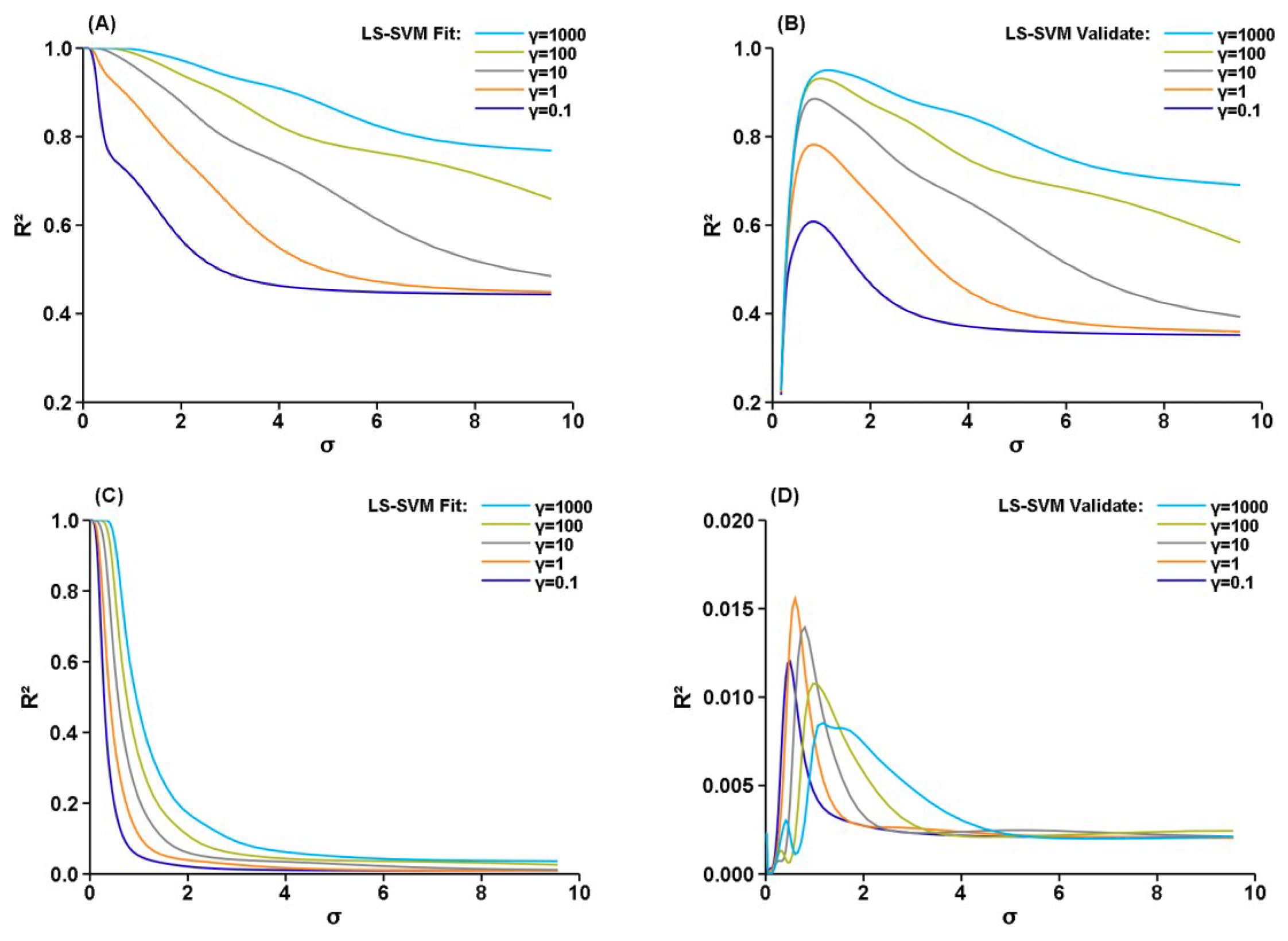
Figure 1 shows the correlation coefficient (R²) between the LS-SVM outputs and the target values of the artificial dataset. In the experiments of Figure 1A,B, five random variables in (−1,1) were used as inputs and the results of Equation (11) as the target. Both the fitting and validation become better with a larger γ. Equation (9) indicates that a larger γ means more precise fit of the data; and the kernel function (6) indicates that a smaller σ yields a larger variability. Therefore, a smaller σ and a larger γ yields a better fitting for the noise-free data. The validation shows that the best fitting did not generalize well. The optimal σ is 1.17 for γ = 1000 and did not stray far from the optimal value for other γ. The experiments in Figure 1C,D used four random variables as input and a random variable in the same range as the target. That the LS-SVM can make a perfect fitting for unrelated variables is an example of overfitting. Although the correlation detected by the validation is weak, σ = 0.6 and γ = 1 are clearly the candidates for obtaining a better validation. Small correlations in the validation resulted from a few random points that incidentally fit Equation (11).

Using the optimal σ value s of the LS-SVM, we conducted grid search for the optimal C and ε of the SVM with the same artificial dataset. For the noise-free target, ε = 0.01 in the discrete set (0.01, 0.02, 0.05, 0.10, 0.20, 0.30) and C = 1000.0 in the discrete set (0.1, 1.0, 10.0, 100.0, 1000.0) yielded the best validation. This is understandable as the target includes no noise, a smaller ε, and a larger C would include more data points as support vectors to produce a better fitting and validation. When the target was a random variable, ε = 0.1 and γ = 1.0 became optimal values.

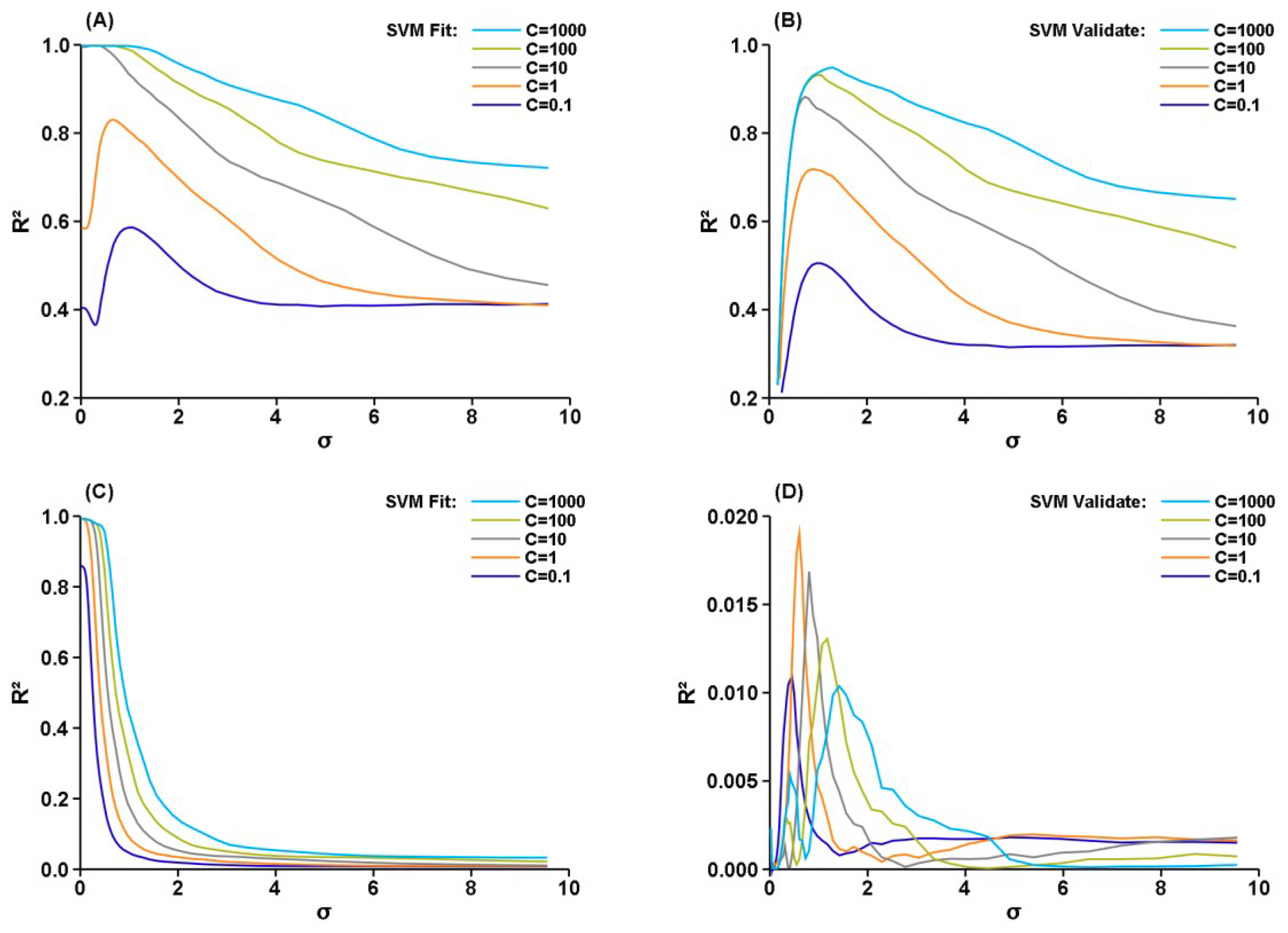
Figure 2 shows that the SVM behaved similar to the LS-SVM. The grid search for the optimal C and σ was done with the optimal ε values above. When the target is noise free, the R² of both fitting and validation increases monotonically with the C parameter (Figure 2A,B) for a given σ. In the fitting, the R² tends to decrease monotonically with the σ for a large C. This is because a large C made LibSVM include most training samples as support vectors and smaller σ makes the hyperplane more elastic. But with a small C, the optimal σ occurred in a narrow range around 1.0, which differs not much from the standard deviation of the target (0.58). In the validation, the optimal σ appeared around 1.0 for all tested C values. Obviously, an over fitting would have occurred with a small σ and a large C, resulting in excellent fitting but unacceptable validation. One may ask what the results would be for C > 1000. The outputs of LibSVM show that nearly all training data points have been included as support vectors; therefore, using larger C would yield similar results as those with C = 1000.

We reassessed the optimal ε value of the SVM for the CO₂ dataset as the target has a much larger variance. Based on the experiments with the random dataset, we set σ = 0.6 to evaluate the ε in the discrete set (1, 2, 4, 8, 16, 32 µatm). Divided by the CO₂ standard deviation of 32.6 µatm, these values correspond to ε of 0.03, 0.06, 0.12, 0.24, 0.49, and 0.98, respectively, for normalized CO₂. Figure 3 shows the variation of the correlation coefficient and bias (model-target) obtained from a validation. Obviously, one cannot have both a zero bias and the best correlation. Our priority is to have a zero bias as a large bias may reverse the conclusion of the global oceans as CO₂ sink or source. Since the bias crosses the zero line for all tested C values (Figure 3B), we selected C = 100 from Figure 3A and estimated ε ≈ 12 µatm from Figure 3B. This value corresponds to ε of 0.37 for normalized CO₂. Note that it is not necessary to calculate the zero-bias ε precisely as the bias would change with a different training and validation dataset. If one emphasizes having the best correlation, then the best ε would be about 8 µatm or 0.24 for normalized CO₂.

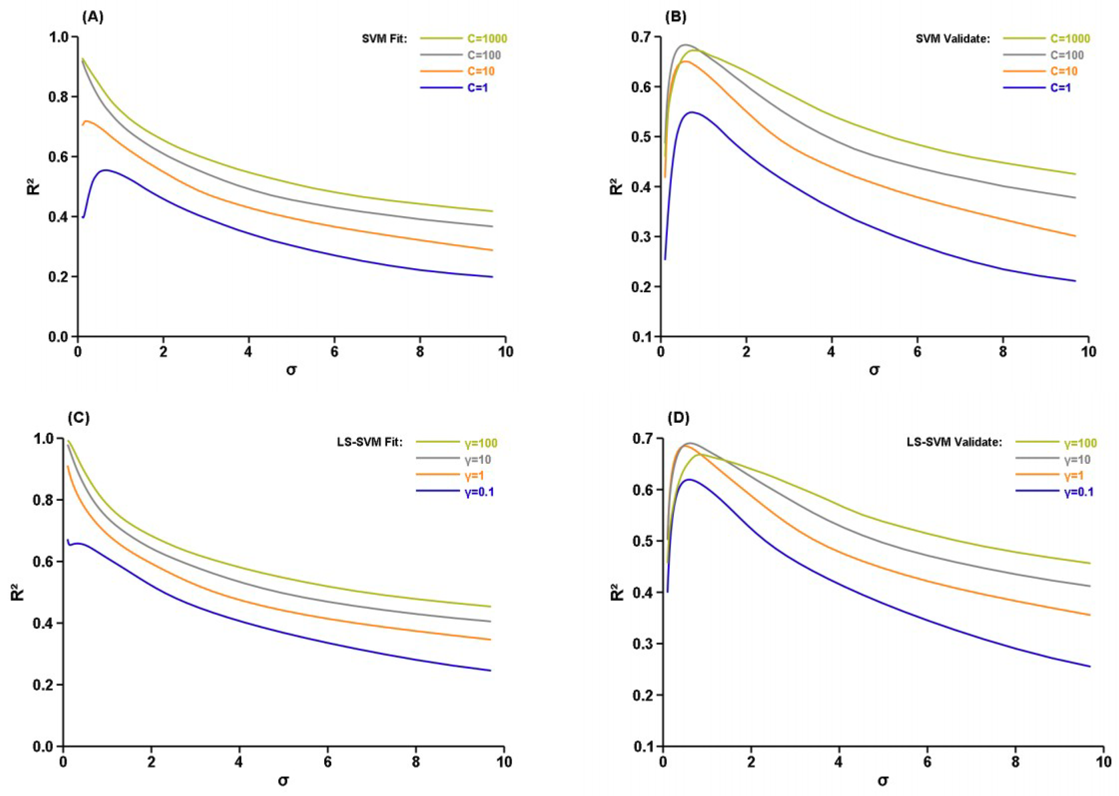
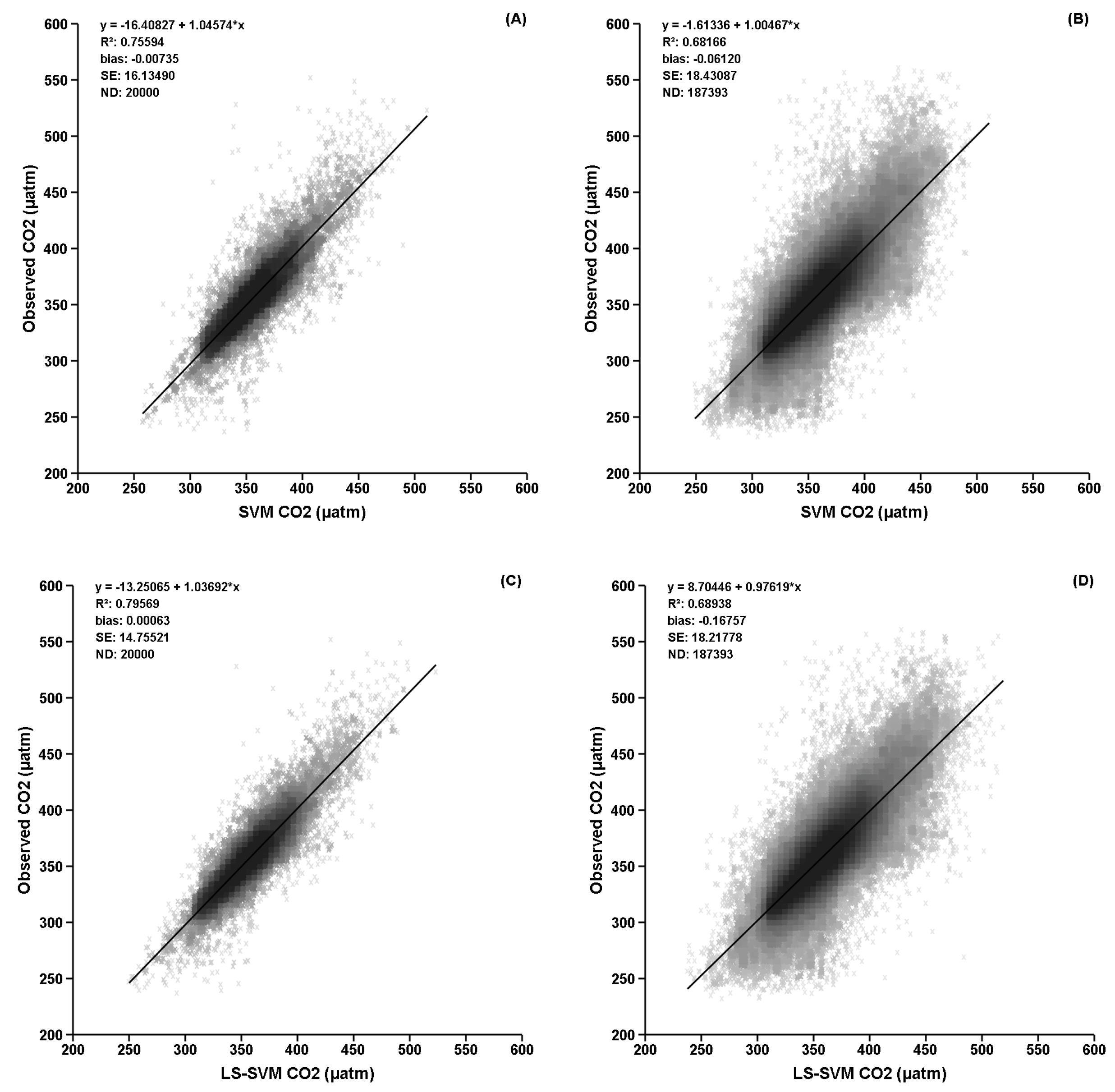
Figure 4 shows the grid search results with ε = 12 using a CO₂ dataset. The optimal C of the SVM is 1000 for fitting and 100 for validation; and the optimal γ of the LS-SVM is 100 for fitting and 10 for validation. It is no surprise that the optimal σ values of the two model are similar: 0.611 for SVM and 0.690 for LS-SVM. Overall, the two models respond to parameter changes similarly. Further, the responses of both models with the CO₂ dataset are similar to those with noise-free artificial dataset in (Figure 1A,B and Figure 2A,B). Figure 5 presents a fitting and validation obtained using the optimal parameters. Beside having a larger R² and a smaller standard error (SE), the LS-SVM visually shows a less dented blank area near CO₂ value of 320 µatm. The skewed distribution of data points around the regression line indicates unbalance sampling of the measurements. The SVM yielded a smaller validation bias because the dataset was used to choose the ε to have a zero-bias validation.

We repeated the grid search for optimal parameters for the 10 CO₂ datasets prepared for Monte Caro cross validation. We obtained the overall optimal C and σ of the SVM as 100 and 0.613, respectively, and optimal γ and σ of the LS-SVM as 10 and 0.695, respectively. The biases in

Table 1. Monte Carlo cross validation of the SVM. Each dataset was derived by randomly sampling 10% of the primary data for training (fitting) and the rest 90% for validation. The goodness of fitting and validation was measured by the squared correlation coefficient between model outputs and target values.

Sample ID	Training R2	Training Bias	Validate R2	Validate Bias
1	0.756	−0.01	0.682	−0.06
2	0.763	−0.03	0.679	0.00
3	0.758	−0.11	0.678	−0.81
4	0.757	−0.02	0.680	−0.38
5	0.764	−0.10	0.681	−0.23
6	0.765	−0.02	0.682	0.06
7	0.770	−0.02	0.680	0.29
8	0.751	−0.07	0.680	−0.12
9	0.762	−0.02	0.680	−0.17
10	0.764	−0.11	0.679	−0.27
Mean	0.761	−0.05	0.680	−0.17
STDEV	0.005	0.05	0.001	0.29

and

Table 2. Monte Carlo cross validation of the LS-SVM. Each dataset was derived by randomly sampling 10% of the primary data for training (fitting) and the rest 90% for validation. The goodness of fitting and validation was measured by the squared correlation coefficient between model outputs and target values.

Sample ID	Training R2	Training Bias	Validate R2	Validate Bias
1	0.796	0.00	0.689	−0.17
2	0.802	0.00	0.693	−0.11
3	0.798	0.00	0.691	−0.42
4	0.795	0.00	0.689	−0.21
5	0.804	−0.00	0.693	−0.16
6	0.804	0.00	0.692	0.02
7	0.807	0.00	0.691	0.09
8	0.793	0.00	0.688	−0.09
9	0.803	0.00	0.689	−0.14
10	0.804	0.00	0.691	−0.16
Mean	0.801	0.00	0.691	−0.14
STDEV	0.005	0.00	0.002	0.14

were obtained using these parameter values. Overall, the LS-SVM performs better than the SVM in terms of correlation and bias. The LS-SVM yielded a mean bias of 0.00 ± 0.00 μatm and −0.14 ± 0.14 μatm for fitting and validation, respectively; and a mean R² of 0.801 ± 0.005 and 0.691 ± 0.002 for fitting and validation, respectively. Whereas, the SVM yielded a mean bias of −0.05 ± 0.05 μatm and −0.17 ± 0.29 μatm for fitting and validation, respectively; and a mean R² of 0.761 ± 0.005 and 0.680 ± 0.001 for fitting and validation, respectively. The SVM yielded a larger variance for both bias and R² as there is no ε that can minimize the bias of all datasets and the number of support vectors changes with different datasets, even using the same C value.

The performance of the two models in term of computing time did not differ much. This was evaluated using a PC with an Intel Xeon 3.20 GHz CPU and 32 GB memory. The LS-SVM took 43 s to complete a training of 20,000 samples. The training time of the SVM increased linearly with C from 7 s for C = 1 to 350 s for C = 1000. While the SVM would take more time to search for support vectors with a more relaxed constrain in Equation (4) or a larger C, the bottleneck of the LS-SVM is in solving Equation (9). In our experiments, the conjugate-gradient method of the LS-SVM software took about 200 to 300 iterations to obtain a solution with a sufficient precision. The number of operations on floating number is about O(iteration × n²) for a n × n matrix, which is much smaller than O(n³) operations of the LU decomposition method, commonly used for solving linear system equations.

The LS-SVM has fewer parameters to be tuned than the SVM. Therefore, it is harder to obtain the optimal parameters of the SVM. However, the resource-thirsty characteristic of the LS-SVM could limit its use with a large dataset. We tested the LS-SVM model with 60,000 training samples. It took 920 s to complete a training, which is not unacceptable. However, it consumed 28.5 GB memory. Increasing the sample size further halted our computer. Meanwhile, the SVM consumed only 130.5 MB memory and the training took 600 s for C = 100.

4. Discussion

Both the SVM and LS-SVM are capable of fitting any data perfectly well, even when there is no relation between the target and the input variables. A good validation setting is critical to obtain optimal parameters to generalize a train model to make meaningful predictions. Although various methods have been proposed for parameter optimization, long computing time could become an obstacle for all the methods with a large dataset. A universally good initial guess for the parameters can accelerate the search for optimal parameters. But it is impossible to obtain universally good initial guesses without data scaling. Many articles have pointed out that data scaling is very import to using the SVM and LS-SVM effectively. Input variables rarely have the same units and changing the units of a variable may change its variation range significantly. The variable having a significantly larger variation range would likely dominate the result of the kernel function. With units removed and data scaled to similar ranges, the optimal parameters become more predictable.

We used two datasets to search for optimal parameters with the intention of generalization. Therefore, we designed an artificial dataset for cases of noise-free targets and extreme noisy targets and used a large data from the real world. As the input variables of the first dataset were randomly generated in the range (−1,1), no scaling was applied. The second dataset included more than 200,000 data points used for the global surface ocean CO₂ reconstruction. The input variables were z-normalized. The results reveal several hints to guide using the models. First, the models are most sensitive to the σ parameters of the kernel function and its optimal value lies in a narrow range around one for scaled inputs. Second, the ε parameter of the SVM affects the bias significantly. Its initial guess should be set to about 10%–20% of the standard deviation of the target. Third, the value of 100 is recommended as the initial guess for the C parameter of the SVM. And lastly, the value of 10 is recommended as the initial guess for the γ parameter of the LS-SVM.

The parameter optimization of [18] scaled input variables to the range (0,1) and yielded similar values for the σ and C parameters of the SVM. Based on these results, we conclude that our results can be generalized to other cases if the input variables are z-normalized. Our results also show that the LS-SVM performs better than the SVM in general. For applications that expect unbiased results, the LS-SVM is strongly recommended. The drawback of the LS-SVM is that it consumes much more computer memory than the SVM.

References

- Lecun, Y.; Bengio, Y.; Hinton, G. Deep learning. Nature 2015, 521, 436–444. [Google Scholar] [CrossRef] [PubMed]
- Ge, J.; Meng, B.; Liang, T.; Feng, Q.; Gao, J.; Yang, S.; Huang, X.; Xie, H. Modeling alpine grassland cover based on MODIS data and support vector machine regression in the headwater region of the Huanghe River, China. Remote Sens. Environ. 2018, 218, 162–173. [Google Scholar] [CrossRef]
- Mehdizadeh, S.; Behmanesh, J.; Khalili, K. Comprehensive modeling of monthly mean soil temperature using multivariate adaptive regression splines and support vector machine. Theor. Appl. Climatol. 2018, 133, 911–924. [Google Scholar] [CrossRef]
- Jang, E.; Im, J.; Park, G.H.; Park, Y.G. Estimation of fugacity of carbon dioxide in the east sea using in situ measurements and geostationary ocean color imager satellite data. Remote Sens. 2017, 9, 821. [Google Scholar] [CrossRef]
- Gregor, L.; Kok, S.; Monteiro, P.M.S. Empirical methods for the estimation of Southern Ocean CO2: Support vector and random forest regression. Biogeosciences 2017, 14, 5551–5569. [Google Scholar] [CrossRef]
- Yang, F.; White, M.A.; Michaelis, A.R.; Ichii, K.; Hashimoto, H.; Votava, P.; Zhu, A.-X.; Nemani, R.R. Prediction of Continental-Scale Evapotranspiration by Combining MODIS and AmeriFlux Data Through Support Vector Machine. IEEE Trans. Geosci. Remote Sens. 2006, 44, 3452–3461. [Google Scholar] [CrossRef]
- Sachindra, D.A.; Huang, F.; Barton, A.; Perera, B.J.C. Least square support vector and multi-linear regression for statistically downscaling general circulation model outputs to catchment streamflows. Int. J. Climatol. 2013, 33, 1087–1106. [Google Scholar] [CrossRef]
- Zeng, J.; Matsunaga, T.; Saigusa, N.; Shirai, T.; Nakaoka, S.I.; Tan, Z.H. Technical note: Evaluation of three machine learning models for surface ocean CO2 mapping. Ocean Sci. 2017, 13, 303–313. [Google Scholar] [CrossRef]
- Cortes, C.; Vapnik, V. Support-vector networks. Mach. Learn. 1995, 20, 273–297. [Google Scholar] [CrossRef]
- Smola, A.J.; Schölkopf, B. A tutorial on support vector regression. Stat. Comput. 2004, 14, 199–222. [Google Scholar] [CrossRef] [Green Version]
- Suykens, J.A.K.; Van Gestel, T.; De Brabanter, J.; De Moor, B.; Vandewalle, J. Least Squares Support Vector Machines; World Scientific: Singapore, 2002; ISBN 981-238-151-1. [Google Scholar]
- Meza, A.M.Á.; Santacoloma, G.D.; Medina, C.D.A.; Dominguez, G.C. Parameter selection in least squares-support vector machines regression oriented, using generalized cross-validation. Rev. DYNA 2011, 171, 23–30. [Google Scholar]
- Cherkassky, V.; Ma, Y. Selection of Meta-Parameters for Support Vector Regression. In Proceedings of the International Conference on Artificial Neural Networks 2002, Madrid, Spain, 28–30 August 2002; Dorronsoro, J.R., Ed.; LNCS. Volume 2415, pp. 687–693. [Google Scholar] [CrossRef]
- Chapelle, O.; Vapnik, V.; Bousquet, O.; Mukherjee, S. Choosing multiple parameters for support vector machines. Mach. Learn. 2002, 46, 131–159. [Google Scholar] [CrossRef]
- Frauke, F.; Christian, I. Evolutionary Tuning of Multiple SVM Parameters. In Proceedings of the ESANN’2004 Proceedings—European Symposium on Artificial Neural Networks, Bruges, Belgium, 27–29 April 2004; pp. 519–524, ISBN 2-930307-04-8. [Google Scholar]
- Glasmachers, T.; Igel, C. Gradient-based adaptation of general gaussian kernels. Neural Comput. 2005, 17, 2099–2105. [Google Scholar] [CrossRef] [PubMed]
- Lendasse, A.; Ji, Y.; Reyhani, N.; Verleysen, M. LS-SVM hyperparameter selection with a nonparametric noise estimator. Robotics 2005, 3697, 625–630. [Google Scholar] [CrossRef]
- Jiang, M.; Wang, Y.; Huang, W.; Zhang, H.; Jiang, S.; Zhu, L. Study on Parameter Optimization for Support Vector Regression in Solving the Inverse ECG Problem. Comput. Math. Methods Med. 2013, 2013, 158056. [Google Scholar] [CrossRef] [PubMed]
- Laref, R.; Losson, E.; Sava, A.; Siadat, M. On the optimization of the support vector machine regression hyperparameters setting for gas sensors array applications. Chemom. Intell. Lab. Syst. 2019, 184, 22–27. [Google Scholar] [CrossRef]
- Zhang, L.; Lei, J.; Zhou, Q.; Wang, Y. Using Genetic Algorithm to Optimize Parameters of Support Vector Machine and Its Application in Material Fatigue Life Prediction. Adv. Nat. Sci. 2015, 8, 21–26. [Google Scholar] [CrossRef]
- De Brabanter, K.; Suykens, J.A.K.; De Moor, B. Nonparametric Regression via StatLSSVM. J. Stat. Softw. 2015, 55. [Google Scholar] [CrossRef]
- Chang, C.-C.; Lin, C.-J. Libsvm. ACM Trans. Intell. Syst. Technol. 2011, 2, 1–27. [Google Scholar] [CrossRef]
- Joachims, T. Making Large-Scale SVM Learning Practical. Advances in Kernel Methods—Support Vector Learning; Schölkopf, B., Burges, J.C.C., Smola, A.J., Eds.; MIT Press: Cambridge, MA, USA, 1998; pp. 169–184. [Google Scholar]
- Collobert, R.; Williamson, R.C. SVMTorch: Support Vector Machines for Large-Scale Regression Problems. J. Mach. Learn. Res. 2001, 1, 143–160. [Google Scholar]
- Zeng, J.; Nojiri, Y.; Landschützer, P.; Telszewski, M.; Nakaoka, S. A global surface ocean fCO2 climatology based on a feed-forward neural network. J. Atmos. Ocean. Technol. 2014, 31, 1838–1849. [Google Scholar] [CrossRef]
- Bakker, D.C.E.; Pfeil, B.; Landa, C.S.; Metzl, N.; O’Brien, K.M.; Olsen, A.; Xu, S. A multi-decade record of high-quality fCO2 data in version 3 of the Surface Ocean CO2 Atlas (SOCAT). Earth Syst. Sci. Data 2016, 8, 383–413. [Google Scholar] [CrossRef]
- Reynolds, R.W.; Rayner, N.A.; Smith, T.M.; Stokes, D.C.; Wang, W. An Improved In Situ and Satellite SST Analysis for Climate. J. Clim. 2002, 15, 1609–1625. [Google Scholar] [CrossRef]
- Boyer, T.P.; Antonov, J.I.; Baranova, O.K.; Coleman, C.; Garcia, H.E.; Grodsky, A.; Sullivan, K.D. World Ocean Database 2013, NOAA Atlas NESDIS 72; Levitus, S., Mishonoc, A., Eds.; NOAA Printing Office: Silver Spring, MD, USA, 2013; 209p. [CrossRef]
- O’Reilly, J.E.; Maritorena, S.; Siegel, D.; O’Brien, M.C.; Toole, D.; Mitchell, B.G.; Culver, M. Ocean color chlorophyll a algorithms for SeaWiFS, OC2, and OC4: Version 4. In SeaWiFS Postlaunch Technical Report Series; SeaWiFS Postlaunch Calibration and Validation Analyses, Part 3; NASA Goddard Space Flight Center: Washington, DC, USA, 2000; Volume 11, pp. 9–23. [Google Scholar] [CrossRef]
- Schmidtko, S.; Johnson, G.C.; Lyman, J.M. MIMOC: A global monthly isopycnal upper-ocean climatology with mixed layers. J. Geophys. Res. Ocean. 2013, 118, 1658–1672. [Google Scholar] [CrossRef] [Green Version]
- Xu, Q.S.; Liang, Y.Z. Monte Carlo cross validation. Chemom. Intell. Lab. Syst. 2001, 56, 1–11. [Google Scholar] [CrossRef]
- Zeng, J.; Nojiri, Y.; Nakaoka, S.; Nakajima, H.; Shirai, T. Surface ocean CO2 in 1990–2011 modelled using a feed-forward neural network. Geosci. Data J. 2015, 2, 47–51. [Google Scholar] [CrossRef]
Figure 1.
Grid search for the optimal γ and σ of the LS-SVM. (A,B) used five random variables in (−1,1) as inputs and the results of Equation (11) as the target. (C,D) used four random variables in (−1,1) as input and a random variable in the same range as the target.
Figure 2.
Grid search for the optimal C and σ of the SVM. (A,B) used five random variables in (−1,1) as input and the results of Equation (11) as the target. (C,D) used four random variables in (−1,1) as inputs and a random variable in the same range as the target.
Figure 3.
Grid search for the optimal C and ε of the SVM model with σ = 0.6. The results were from the validation of a CO2 dataset. Obviously, one cannot have both zero bias and the best correlation. (A) Variation of correlation coefficient; (B) Variation of bias.
Figure 4.
Grid search for optimal parameters of the SVM and LS-SVM models using a CO2 dataset. Both models respond to parameter changes similarly. (A) SVM fitting; (B) SVM validation; (C) LS-SVM fitting; (D) LS-SVM validation.
Figure 5.
Scatter plots of modeled vs observed CO2 concentrations. Uneven distribution of points indicates unbalance sampling in different ocean domains. The darker the color, the denser the sample points. The LS-SVM yielded a larger R2 and smaller SE than the SVM did. The SVM yielded a smaller validation bias because the dataset was used to choose the ε to have a zero-bias validation. (A) SVM fitting; (B) SVM validation; (C) LS-SVM fitting; (D) LS-SVM validation.