Article

Data Mining Algorithms for Operating Pressure Forecasting of Crude Oil Distribution Pipelines to Identify Potential Blockages

by
Agus Santoso
1,*,
Fransisco Danang Wijaya
1,
Noor Akhmad Setiawan
1 and
Joko Waluyo
2
1
Department of Electrical and Information Engineering, Universitas Gadjah Mada Yogyakarta, Yogyakarta 55281, Indonesia
2
Department of Mechanical and Industrial Engineering, Universitas Gadjah Mada Yogyakarta, Yogyakarta 55284, Indonesia
*
Author to whom correspondence should be addressed.
Mach. Learn. Knowl. Extr. 2022, 4(3), 700-714; https://doi.org/10.3390/make4030033
Submission received: 22 June 2022 / Revised: 13 July 2022 / Accepted: 19 July 2022 / Published: 21 July 2022
(This article belongs to the Section Learning)

Abstract

:
The implementation of data mining has become very popular in many fields recently, including in the petroleum industry. It is widely used to help in decision-making processes in order to minimize oil losses during operations. One of the major causes of loss is oil flow blockages during transport to the gathering facility, known as the congeal phenomenon. To overcome this situation, real-time surveillance is used to monitor the oil flow condition inside pipes. However, this system is not able to forecast the pipeline pressure on the next several days. The objective of this study is to forecast the pressure several days in advance using real-time pressure data, as well as external factor data recorded by nearby weather stations, such as ambient temperature and precipitation. Three machine learning algorithms—multi-layer perceptron (MLP), long short-term memory (LSTM), and nonlinear autoregressive exogenous model (NARX)—are evaluated and compared with each other using standard regression evaluation metrics, including a steady-state model. As a result, with proper hyperparameters, in the proposed method of NARX with MLP as a regressor, the NARX algorithm showed the best performance among the evaluated algorithms, indicated by the highest values of R2 and lowest values of RMSE. This algorithm is capable of forecasting the pressure with high correlation to actual field data. By forecasting the pressure several days ahead, system owners may take pre-emptive actions to prevent congealing.

1. Introduction

The implementation of data mining techniques in the petroleum industry has become very popular recently, and it can support decision-making processes to optimize various operational aspects [1,2]. One of the crucial operational aspects in the petroleum industry is flow assurance in oil pipeline systems, a lack of which can lead to massive oil losses; for example, the congeal problem is caused when oil shifts from liquid to solid phase [3,4], creating restrictions or blockages of the oil flow (see Figure 1). The oil losses due to congeal events may be worth millions of US dollars; furthermore, the actions required to solve such problems might also cost millions of US dollars [5,6,7,8,9]. Therefore, accurately predicting the pressure several days ahead is crucial for the efficient prevention of oil losses.
The congeal phenomenon becomes worse in mature oil fields, as the fluid temperature has been decreasing due to the naturally declining fluid reservoir temperature [10]. This decreased temperature may lead the fluid temperature to approach the wax appearance temperature (WAT), which initiates the congeal phase [11,12]. To avoid congealing, several actions could be taken, such as insulation installation, regular pigging, and chemical injection [13,14]. One of the most common types of chemical inhibitor is pour point depressants (PPDs), which prevent wax formation even when the fluid temperature reaches the WAT [15]. An online monitoring system is usually deployed to monitor the congeal phenomenon by observing the flow pressure inside the pipeline, as well as other parameters [16]. By having real-time pressure data, a field operator could take preventive action for a specific segment of pipeline. However, by relying on real-time measurements only, the preventive actions may be too late: the congeal event has already started, while the operators require time for preparation and the chemical also takes time to reach the target point. Therefore, forecasting of pressure several days ahead is highly required, in order to help the operation team to combat the congeal problem.
To date, research on congeal prediction has been carried out by many researchers in order to predict wax deposition using static data obtained from controlled experiments [17,18,19,20,21,22]. On the other hand, the pressure in a real pipeline system in the field is dynamic; therefore, the experimental results obtained using static data cannot be directly implemented in the field. In this research, we apply data mining algorithms to predict the operating pressure of crude oil distribution pipelines several days in advance using real historical data from the oil field. The contributions of this research are as follows:
  • We propose a novel approach using data mining techniques to address the congeal problem using common real-time surveillance measurements from oilfields;
  • We provide a data set from an oil pipeline system in an actual oilfield. This data set is available to other researchers for future work.

2. Materials and Methods

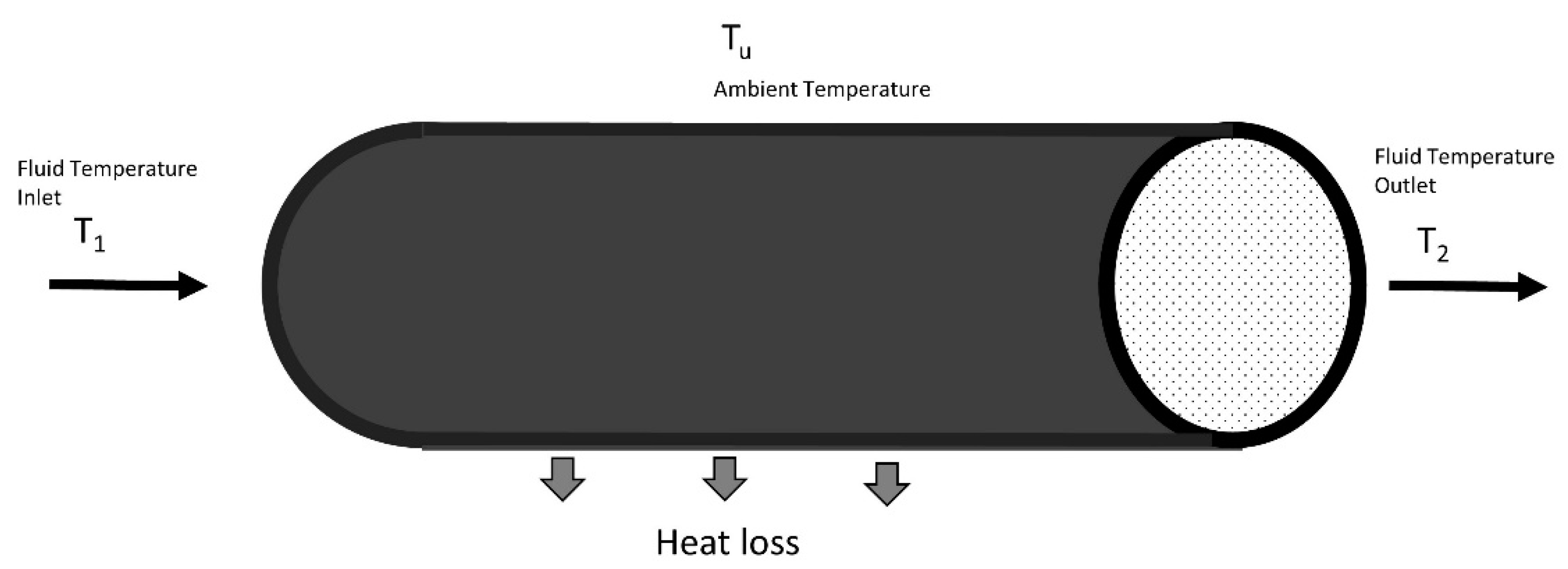
2.1. The Operation under Study

All parameters were taken from the upstream of a 10-inch-diameter crude oil shipping line that is located at Central Sumatera Operation, Indonesia. The total pipe length is around 9 km, and it is mainly above the ground. This pipeline is directly exposed to the external environment, with an average ambient temperature of around 80–100 °F and precipitation of 0–15 mm/day, varying with the time of year.
The crude oil is categorized as a light oil with WAT around 130 deg F, and the average oil flow rate inside the pipeline is around 3000 barrels per day. In current practice, four conditions are defined to reflect the congeal condition: normal, caution, near congeal, and congeal. These conditions were derived from physics-based simulations according to data from laboratory experiments. As shown in Table 1, the operations team will take action to prevent congealing from happening when the pressure status is not normal (i.e., higher than 154 psi).
Regarding the data used for modeling, real-time pressure measurements, along with external factors such as ambient temperature and precipitation rate, are historically available from the sensor and local weather stations. For future use of external factors during prediction, weather forecasts from a weather service provider can also be utilized. Therefore, future data of external factors can be used as additional inputs for the future pressure forecast. Figure 2 depicts the information of historical parameters, available from real field measurements. It can be clearly seen that the ambient temperature has a significant impact on the behavior of the incoming pressure system, as indicated by major fluctuations in the incoming pressure being inversely proportional to the ambient temperature.
As the oil is shipped from the gathering station, the fluid temperature decreases along the shipping line due to heat transfer from the fluid inside the pipe to the surrounding environment. Typically, the incoming fluid temperature from the gathering station is around 143 °F, while the ambient temperature falls within the range from 70 to around 90 °F. This temperature difference enables heat to move toward the surrounding environment through the pipe, as shown by the illustration of the radial heat transfer process in Figure 3.
The temperature drop becomes bigger when the ambient temperature is low, for example, during rain, as shown by the equation below:
T 2 = T u + ( T 1 T u )   e x p [ U π d m C p L ]
where T2 is the fluid outlet temperature, Tu is the ambient temperature, T1 is the fluid inlet temperature, U is the transmission coefficient, d is the pipe diameter, m is the mass flowrate, Cp is the fluid head capacity, and L is the length of pipe. It can be observed that ambient temperatures impact the overall temperature profile along the pipeline, as illustrated by Figure 4.
When the fluid temperature reaches the Wax Appearance Temperature (WAT), the wax starts to form deposits and stick to the wall of the pipe. In addition, the decreasing temperature also impacts the oil viscosity, creating flow restriction and leading to lower fluid flow. According to the RRR (Rygg, Rydahl, and Ronningsen) model, wax deposition is driven by molecular diffusion and shear dispersion. In addition, decreasing flowrate will accelerate the wax thickening process. When all this happens in the shipping line system, the incoming pressure will increase significantly due to the back pressure created by the reduced effective diameter or the blockage inside the pipeline. Thus, in the worst case, the fluid will stop flowing, potentially leading to loss-of-containment issues due to pipeline leakage. Precipitation is also included to help in predicting future pressure changes.

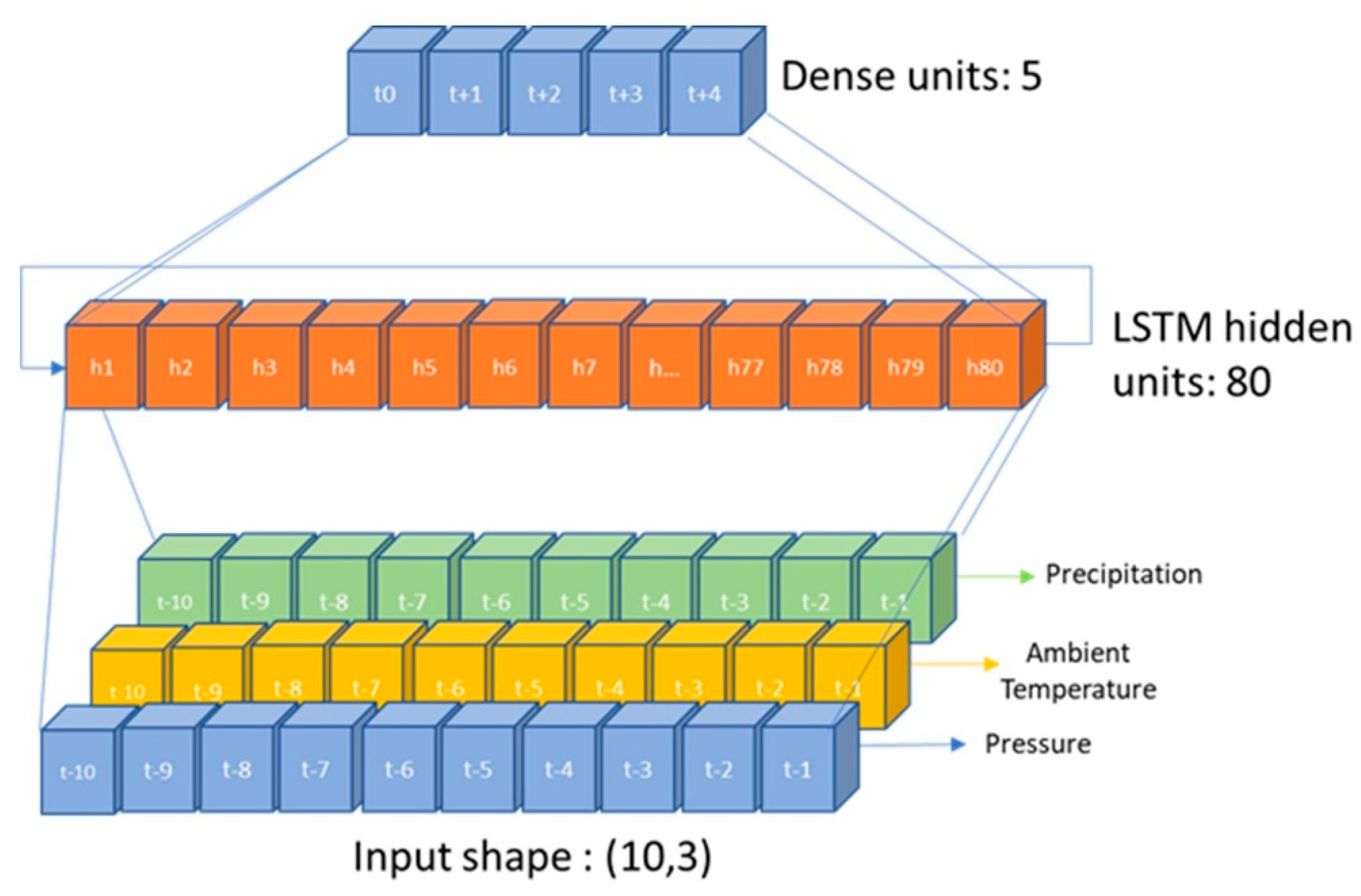
2.2. Machine Learning Algorithms

For this research, three machine learning algorithms specifically for regression were selected. The first method is the backpropagation MLP, which mimics the concept of the human brain. This algorithm is very robust and can determine the nonlinear correlations between the input and output. It consists of three types of layers: input, hidden, and output. The general operation, involving synaptic weights and input, can be described as:
v = w 0 x 0 + i 1 = 1 n w i 1 x i 1 ,
where xi denotes neuron input i, wi denotes the weight of neuron input i, x0 is the bias neuron input, w0 is the weight of the bias, and v is the output of the synaptic operation. The somatic operation to calculate the outputs can be described as:
y = φ ( v ) ,
where y is the output of the respective neuron and φ is the activation function. In this approach, the inputs come from the feature engineering process in order to generate new features, such as time features (day of week, day of month, month) and statistical features (slope, max, min, average), of the pressure and external factors. In this study, MLP was used to predict multiple-output pressure directly for five consecutive days.
The second algorithm is the long short-term memory (LSTM) network, a variant of the recurrent neural network (RNN). One signature feature of the RNN-family algorithms is the use of network delay recursion. This approach is very suitable when considering time-series data. The delayed signal allows the model to “remember” the signal before time t. Even though this memory delay capability is very robust for short-term signals, the RNN lacks long-term memory. Another disadvantage of the RNN is the vanishing gradient problem. These weaknesses are addressed by LSTM, which utilizes a memory cell in order to retain long-term dependencies. The main feature of LSTM is the cell state (memory cell), as described in Figure 5.
During training, the cell state is managed by structure gates. There are three gates controlling the cell state. The first gate removes unused information from the memory cell with the following equation:
f t =   σ (   W f × x t + U f × h t 1 + b f ) ,
where f t denotes the decision of whether information is to be removed from the cell state, σ denotes the sigmoid activation function, W f and U f are weight vectors, x t is the neuron input, h t 1 is the cell output at the previous time step (t − 1), and b f is the bias.
The second gate is the input gate, which determines which information is input at the current time t. This gate enables the output value to be updated. Then, a layer with tanh as the activation function generates a new cell state value, C ˜ t . The input gate can be defined as:
i t =   σ (   W i × x t + U i × h t 1 + b i ) ,
C ˜ t =   tanh ( W c × x t + U c × h t 1 + b c ) ,
where i t denotes the decision regarding which information is updated; W i , U i , W c , and U c are the weights of the network; and b i and b c are bias terms. Then, the new cell state of C t is defined as
C t = C t 1 × f t + i t × C ˜ t .
The third gate is the output gate, which defines the output information at the current time t. The output gate can be denoted as:
O t =   σ ( W o × x t + U o × h t 1 + b o ) ,
where O t denotes the decision of what information is to be output, W o and U o are weight vectors, and b o is the bias term. The cell output can be denoted as:
h t = O t × tanh ( C t ) ,
where h t specifies the cell value at time t.
The third algorithm is the nonlinear autoregressive with exogenous inputs (NARX) model, a recurrent dynamic neural network that utilizes feedback connections to several layers of the network. To capture nonlinear behavior, MLP is used as a regressor. The NARX architecture allows external factors and their lagged versions to be used as the inputs. The pressure forecasted at the next step is also used to predict the following step recursively. The NARX algorithm was also adopted in another research [21].

2.3. Performance Evaluation

In this research, common regression performance metrics are used, such as R2 (the coefficient of determination) and the root-mean-square error (RMSE), defined as follows:
R 2 = 1 i = 0 n 1 ( y i y ^ i ) 2 i = 0 n 1 ( y i y ¯ ) 2 ,
R M S E = 1 n i = 0 n 1 ( y i y ^ i ) 2 ,
where y i is the actual target for component i, y ^ i is the predicted value, y ¯ is the mean value, and n denotes the amount of data.

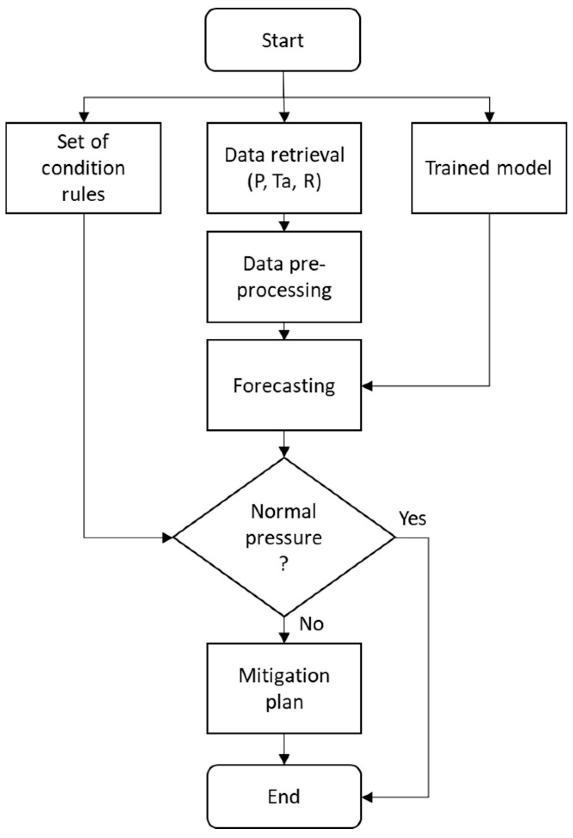
2.4. Framework of the Evaluated Models

The data used are of daily frequency, including the first 720 data as training data and the last 180 days as a blind data set. The completed dataset is provided in Supplementary Materials. Each of three modelling approaches was evaluated based on their R2 and RMSE values on the blind data set.
The first approach was the MLP-based model, using engineered features as inputs to the model. Some of features were derived from time information, such as day of week, day of month, and month. The other features were derived from simple rolling calculations in certain time windows, such as min, max, average, and slope, for all three series of data in the field measurements. Based on experiments, three days of rolling calculation was the best choice to predict pressure in the system being observed. In addition, these simple calculations were applied to the future values of external factors: as described previously, future external factors were accessible from the weather service provider. In total, there were 23 parameters used by the MLP, as described in Table 2.
The topology of the MLP algorithm used in this research was defined as having 23 total input features, 1 hidden layer with 30 hidden neurons initially, the ReLU activation function, and a selected learning rate of 0.0001. These hyperparameters were selected based on a trial-and-error process considering different combinations of hyperparameters.
The second approach, based on LSTM, used inputs from the lagged versions of the pressure and external factors. The number of lags used in this study was 10, while the model had 80 hidden neurons, as shown in Figure 6. These parameters were selected based on a trial-and-error process. In this approach, no future external factors were used to predict future pressure.
The last approach was based on NARX-MLP, which used lagged inputs of pressure and external factors. Based on a trial-and-error process, the selected order of hyperparameters was 10 for all three data series. Future external factors were also used to predict future pressure, as shown in Figure 7.
The most accurate method was chosen as the final model, to be combined with a set of conditions to predict the congeal status. Based on the status for the next five consecutive days, the operator could take appropriate actions to prevent congeal events that might happen in the future, based on the recommendation of the system. The details of the system are depicted in Figure 8.

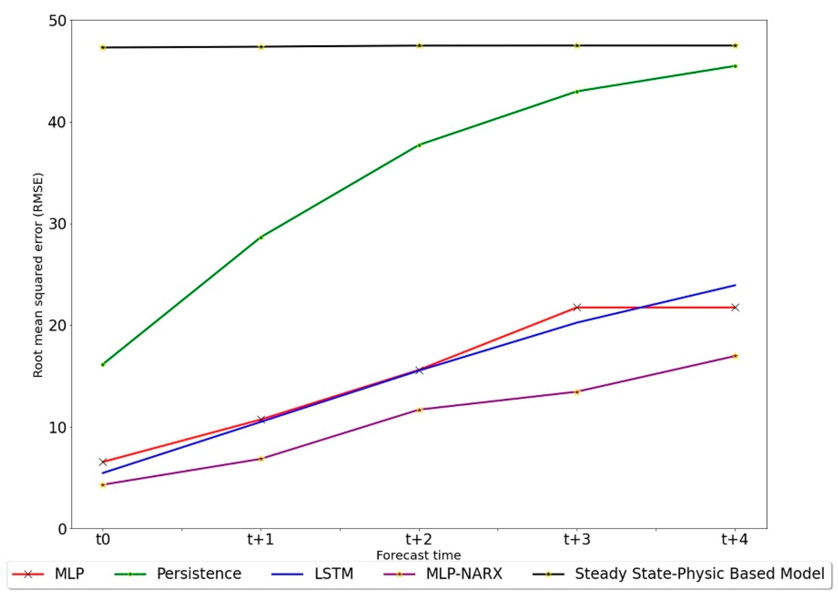
3. Results and Discussion

A comparison of the three proposed models and persistence is presented in Figure 9. In addition, the steady-state simulator result is also provided on the chart. The evaluation was made based on the blind data set.
The figure shows that all machine learning models significantly outperformed both the persistence and the steady-state simulator. Since the steady-state system uses the historical data at one particular time, the prediction of pressure values for all time steps is the same in this evaluation process. A comparison of the first step of prediction between NARX-MLP and the steady-state simulator is depicted in Figure 10. It can be clearly seen that the simulator was too optimistic in predicting high pressure in a more frequent way. Therefore, the simulator would trigger too many alarms that would be used as an indicator to start chemical injection into the shipping line. By having a more accurate model, the chemical injections used in the oil congeal prevention program can hopefully be reduced, saving several hundred thousand USD ($150.000 USD per year).
In terms of individual machine learning model performance, NARX-MLP was the best model, followed by LSTM and MLP, in that order, for all steps ahead. However, the LSTM model, as described previously, did not include future values of external factors, which should be considered in future works. All of the models had similar behavior in general, in that the error increased as the prediction step moved further from the current time step. The detailed performance of NARX-MLP, which was the best model, on the blind dataset is visualized in Figure 11, Figure 12, Figure 13, Figure 14 and Figure 15. As the forecast horizon increases, the prediction deviates from the perfectly fitted line, which is indicated by dotted black line. This means that for a longer forecast horizon, the prediction of high-pressure values tends to be pessimistic, while the prediction of low-pressure values tends to be optimistic. Table 3 summarizes the RMSE and R2 values for NARX-MLP prediction on the blind data set.
As explained by an evaluation study on the different types of forecasting strategy [22], recursive strategies have a major drawback in long-horizon forecasting due to forecast error accumulation in the absence of a corrective mechanism. In a recursive strategy, the model is basically fitted based on one-step-ahead forecasting so that the single model parameter is used for all forecast horizons. To add a corrective mechanism, a multi-step recursive strategy, as mentioned in the previous work [22], could potentially be used for future work so that each time step has different model parameters. In order to manage the effect of the recursive method’s limitations during implementation, a protocol can be applied by the decision maker to pay attention not only to forecast magnitude but also to forecast direction.
As detecting the actual high pressure is critical, a different threshold could be used for each time step such that a longer-horizon forecast will have a lower threshold, especially for the near-congeal condition. Since the model was built based on a relatively small dataset of around 3 years (as compared to the age of the field, which has been producing for more than 52 years), the dataset used in this study does not cover the overall trends as an effect of natural field decline. Therefore, a prior probability shift, which is a change in the target variable, could violate the basic assumptions of the ML model that the past data represent the future ones. However, a significant change in data requires quite a long time, so the model in this study is expected to perform well for several years ahead with regular monitoring of the model performance, for example, by using a set of statistical calculations.
In addition, an engineering assessment should be carried out before making a decision since the model has limited ability to extrapolate, for example, the potential of performance deviation during a shutdown event, since the model was built based on the data of a running system. For long-term application of the model in solving the congeal problem, further study should be conducted to overcome the potential of target change in the future, as well as the reduced congeal problem events, since the shipping line system has been exposed to proactive congeal prevention that minimizes the number of high-pressure events in the data. A physics-guided machine learning approach is probably useful to overcome this problem and to model long-term change in the trend.
The forecast of NARX-MLP, as compared to the actual line plot, is shown in Figure 16. The thresholds are overlaid, which indicates congeal status during the operations. The figure implies that, during operations, pressure only reached the watchful area (i.e., below the yellow line). Therefore, the model was not exposed to data above the yellow line, such that evaluation in more critical areas, such as near-congeal conditions, did not need to be performed.
According to the above results, the machine learning models that were used in this study showed a capability to provide better forecasts, when compared to the persistence, even when using a limited amount of measured data from the field. By using daily data from real-time measurements along with historical values, the models can well-capture the dynamic behavior of the pressure system, as compared to commercial software which assumes that the system is in steady-state conditions. The best model was based on the NARX-MLP model, which could predict especially accurately for the first two steps ahead; however, there is much room for improvement in future works, in terms of obtaining more accurate predictions from the third step onward. The LSTM also showed good potential for use in this kind of problem, as the model used in this study did not take future values of external factors into account in the pressure forecast. We also demonstrated a simple yet applicable approach in applying machine learning to solve congeal events—serious real-world problems—using data commonly obtained in oil fields. In addition, by combining existing knowledge with the models proposed in this study, the process owner could be assisted in making better decisions.

4. Conclusions

Congealing is one of the biggest problems in oil fields, leading to major oil losses in the petroleum industry. Even though the fields are commonly equipped with online field monitoring equipment, the process owner cannot react fast enough when considering real-time data, as mitigation plans require some amount of time for execution and preparation, as well as considering the travel time of the chemical to the target point. By applying machine-learning-based models for pressure system forecasting, the operator may have enough time to adequately prepare a mitigation plan. However, this is still limited by model accuracy, especially in terms of predicting further time steps. For longer pipelines that require higher accuracy, especially in further time steps, improved model performance is essential.
Three machine learning algorithms—multi-layer perceptron (MLP), long short-term memory (LSTM), and the nonlinear autoregressive exogenous model (NARX)—were evaluated in this paper and compared with each other using standard regression evaluation metrics. As a result, with proper hyperparameters, in the proposed method of NARX with MLP as a regressor, the NARX algorithm showed the best performance among the evaluated algorithms, indicated by the highest values of the coefficient of determination (R2) and lowest values of the root-mean-square error (RMSE). Therefore, comparing the three models introduced in this paper, the NARX-MLP outperformed MLP and LSTM in all steps ahead.
The pressure prediction for t0 using NARX-MLP had relatively high accuracy, as shown by the small RMSE value of 4.29 and high R2 value of 0.96. The values indicate that the NARX-MPL algorithm is capable of forecasting the pressure with high correlation to actual field data. By forecasting the pressure several days ahead, system owners may take pre-emptive actions to prevent congealing. For future work, the data provided can be evaluated using more advanced techniques, particularly to improve forecasting with longer horizons.

Supplementary Materials

The following supporting information can be downloaded at: https://www.mdpi.com/article/10.3390/make4030033/s1, Spreadsheet S1: Field data.

Author Contributions

Conceptualization, A.S., N.A.S., F.D.W. and J.W.; methodology, A.S., F.D.W. and N.A.S.; software, A.S. and N.A.S.; validation, N.A.S., F.D.W. and J.W.; formal analysis, N.A.S. and F.D.W.; investigation, N.A.S. and F.D.W.; resources, A.S., N.A.S. and F.D.W.; data curation, N.A.S. and F.D.W.; writing—original draft preparation, A.S., F.D.W. and N.A.S.; writing—review and editing, N.A.S. and F.D.W. visualization, N.A.S. and F.D.W. supervision, N.A.S., F.D.W. and J.W.; project administration, A.S., N.A.S. and F.D.W. All authors have read and agreed to the published version of the manuscript.

Funding

This research received no external funding.

Institutional Review Board Statement

Not applicable.

Informed Consent Statement

Not applicable.

Data Availability Statement

Not applicable.

Acknowledgments

We thank several people who provided support to this research: Joko Nugroho Prasetyo, Suharyanto, Ramdhan Ari Wibawa, Chairul Ichsan, and Yusuf Hermawan.

Conflicts of Interest

The authors declare no conflict of interest.

References

  1. Obanijesu, E.O.; Omidiora, E.O. Artificial neural network’s prediction of wax deposition potential of Nigerian crude oil for pipeline safety. Pet. Sci. Technol. 2008, 26, 1977–1991. [Google Scholar] [CrossRef]
  2. Wang, Z.; Li, J.; Zhang, H.-Q.; Liu, Y.; Li, W. Treatment on oil/water gel deposition behavior in non-heating gathering and transporting process with polymer flooding wells. Environ. Earth Sci. 2017, 76, 1–15. [Google Scholar] [CrossRef]
  3. ZWang, Z.; Bai, Y.; Zhang, H.; Liu, Y. Investigation on gelation nucleation kinetics of waxy crude oil emulsions by their thermal behavior. J. Pet. Sci. Eng. 2019, 181, 106230. [Google Scholar] [CrossRef]
  4. Zhu, C.; Liu, X.; Xu, Y.; Liu, W.; Wang, Z. Determination of boundary temperature and intelligent control scheme for heavy oil field gathering and transportation system. J. Pipeline Sci. Eng. 2021, 1, 407–418. [Google Scholar] [CrossRef]
  5. Guozhong, Z.; Gang, L. Study on the wax deposition of waxy crude in pipelines and its application. J. Pet. Sci. Eng. 2010, 70, 1–9. [Google Scholar] [CrossRef]
  6. Banki, R.; Hoteit, H.; Firoozabadi, A. Mathematical formulation and numerical modeling of wax deposition in pipelines from enthalpy—porosity approach and irreversible thermodynamics. Int. J. Heat Mass Transf. 2008, 51, 3387–3398. [Google Scholar] [CrossRef]
  7. Moradi, G.; Mohadesi, M.; Moradi, M.R. Prediction of wax disappearance temperature using artificial neural networks. J. Pet. Sci. Eng. 2013, 108, 74–81. [Google Scholar] [CrossRef]
  8. Wang, W.; Huang, Q. Prediction for wax deposition in oil pipelines validated by field pigging. J. Energy Inst. 2014, 87, 196–207. [Google Scholar] [CrossRef]
  9. Behbahani, T.J.; Beigi, A.A.M.; Taheri, Z.; Ghanbari, B. Investigation of wax precipitation in crude oil: Experimental and modeling. Petroleum 2015, 1, 223–230. [Google Scholar] [CrossRef] [Green Version]
  10. Ren, Z.; Cui, J.; Qi, K.; Yang, G.; Chen, Z.; Yang, P.; Wang, K. Control effects of temperature and thermal evolution history of deep and ultra-deep layers on hydrocarbon phase state and hydrocarbon generation history. Nat. Gas Ind. B 2020, 7, 453–461. [Google Scholar] [CrossRef]
  11. Ragunathan, T.; Husin, H.; Wood, C.D. Wax formation mechanisms, wax chemical inhibitors and factors affecting chemical inhibition. Appl. Sci. 2020, 10, 479. [Google Scholar] [CrossRef] [Green Version]
  12. Bell, E.; Lu, Y.; Daraboina, N.; Sarica, C. Experimental Investigation of active heating in removal of wax deposits. J. Pet. Sci. Eng. 2021, 200, 108346. [Google Scholar] [CrossRef]
  13. Labes-Carrier, C.; Rønningsen, H.P.; Kolnes, J.; Leporcher, E. Wax Deposition in North Sea Gas Condensate and Oil Systems: Comparison between Operational Experience and Model Prediction. In Proceedings of the SPE Annual Technical Conference and Exhibition, San Antonio, TX, USA, 29 September 2002; pp. 2083–2094. [Google Scholar] [CrossRef]
  14. Jalalnezhad, M.J.; Kamali, V. Development of an intelligent model for wax deposition in oil pipeline. J. Pet. Explor. Prod. Technol. 2016, 6, 129–133. [Google Scholar] [CrossRef] [Green Version]
  15. Theyab, M.A. Wax deposition process: Mechanisms, affecting factors and mitigation methods. Open Access J. Sci. 2018, 2, 109–115. [Google Scholar] [CrossRef] [Green Version]
  16. Kelechukwu, E.M.; Al-Salim, H.S.; Saadi, A. Prediction of wax deposition problems of hydrocarbon production system. J. Pet. Sci. Eng. 2013, 108, 128–136. [Google Scholar] [CrossRef]
  17. Firmansyah, T.; Rakib, M.A.; George, A.; Al Musharfy, M.; Suleiman, M.I. Transient cooling simulation of atmospheric residue during pipeline shutdowns. Appl. Therm. Eng. 2016, 106, 22–32. [Google Scholar] [CrossRef]
  18. Chu, Z.-Q.; Sasanipour, J.; Saeedi, M.; Baghban, A.; Mansoori, H. Modeling of wax deposition produced in the pipelines using PSO-ANFIS approach. Pet. Sci. Technol. 2017, 35, 1974–1981. [Google Scholar] [CrossRef]
  19. Kamari, A.; Mohammadi, A.H.; Bahadori, A.; Zendehboudi, S. A reliable model for estimating the wax deposition rate during crude oil production and processing. Pet. Sci. Technol. 2014, 32, 2837–2844. [Google Scholar] [CrossRef]
  20. Hu, Z.; Wu, M.; Hu, K.; Liu, J. Prediction of Wax Deposition in an Insulation Crude Oil Pipeline. Pet. Sci. Technol. 2015, 33, 1499–1507. [Google Scholar] [CrossRef]
  21. De Araújo, R.P.; De Freitas, V.C.G.; De Lima, G.F.; Salazar, A.O.; Neto, A.D.D.; Maitelli, A.L. Pipeline inspection gauge’s velocity simulation based on pressure differential using artificial neural networks. Sensors 2018, 18, 3072. [Google Scholar] [CrossRef] [Green Version]
  22. Ben Taieb, S.; Atiya, A.F. A Bias and Variance Analysis for Multistep-Ahead Time Series Forecasting. IEEE Trans. Neural Netw. Learn. Syst. 2016, 27, 62–76. [Google Scholar] [CrossRef] [PubMed]
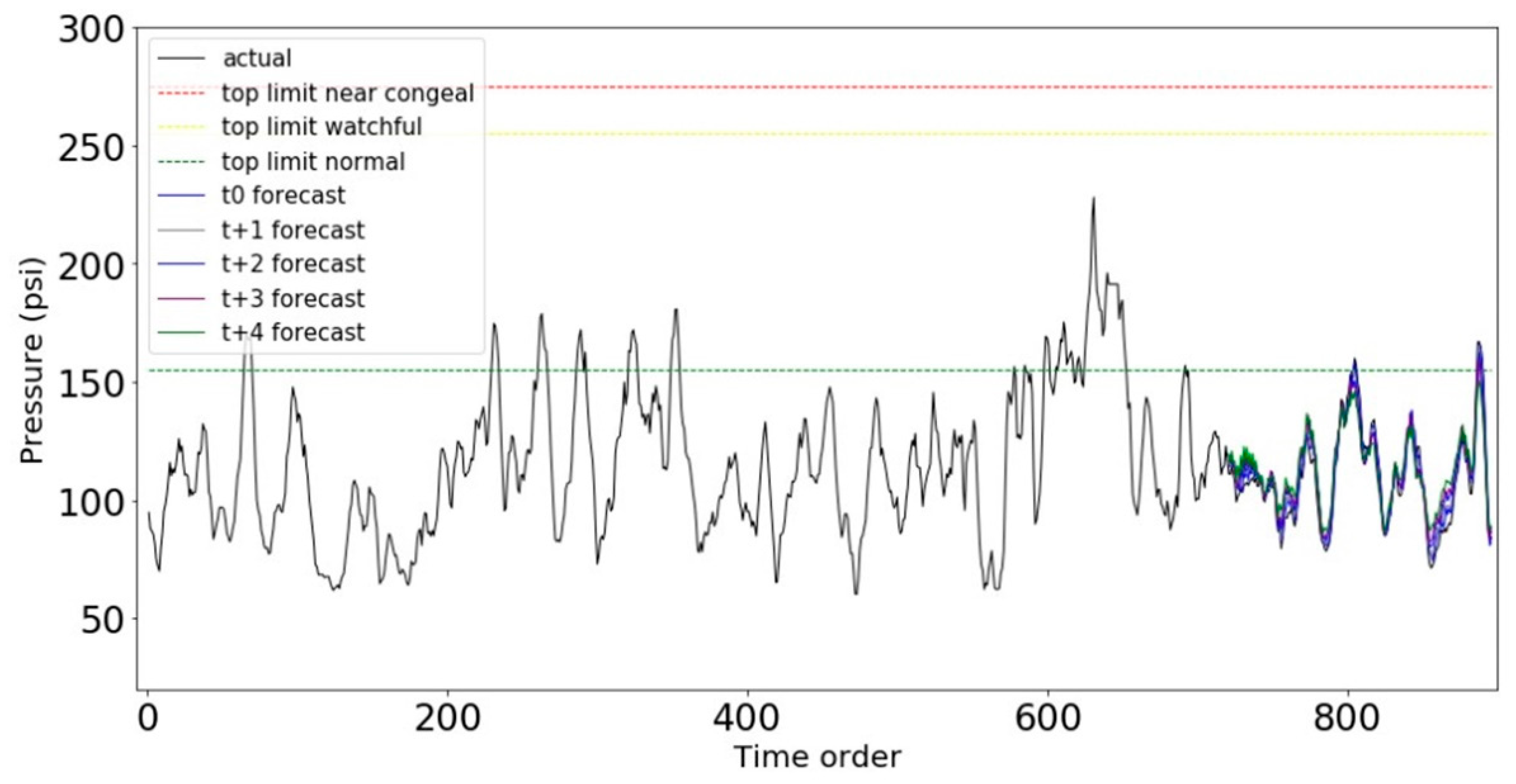
Figure 1. Congeal fluid phenomenon: (a) inside a cut pipeline and (b) solid phase.
Make 04 00033 g001
Figure 2. Historical data of operating pressure, ambient temperature, and precipitation.
Make 04 00033 g002
Figure 3. Radial temperature profile in the pipeline.
Make 04 00033 g003
Figure 4. Schematic of temperature along the pipeline.
Make 04 00033 g004
Figure 5. LSTM cell structure.
Make 04 00033 g005
Figure 6. Structure of the LSTM algorithm.
Make 04 00033 g006
Figure 7. NARX architecture with MLP as the regressor to predict pressure for five consecutive days.
Make 04 00033 g007
Figure 8. Flowchart of the congeal prevention advisory system.
Make 04 00033 g008
Figure 9. RMSE evaluation for the three proposed models and persistence.
Make 04 00033 g009
Figure 10. t0 forecast comparison between the steady state, MLP NARX, and actual.
Make 04 00033 g010
Figure 11. NARX pressure forecasting for t0.
Make 04 00033 g011
Figure 12. NARX pressure forecasting for t + 1.
Make 04 00033 g012
Figure 13. NARX pressure forecasting for t + 2.
Make 04 00033 g013
Figure 14. NARX pressure forecasting for t + 3.
Make 04 00033 g014
Figure 15. NARX pressure forecasting for t + 4.
Make 04 00033 g015
Figure 16. NARX-MLP forecasting plot overlaid with the ground truth and congeal status thresholds.
Make 04 00033 g016
Table 1. Congeal status, referring to pressure at each location.
StatusPressure Range (psi) Color CodeMitigation Action
Normal<155GreenNone
Caution155–255YellowIncrease flowrate from additional well
Near congeal255–275 RedInject chemical (PPD)
Congeal>275BlackShut off operation and combat congealing
Table 2. Inputs and outputs used by the MLP model.
StatusPressure Range (psi)
Day of week
Day of month
Month
Min of pressure of previous 3 days
Max of pressure of previous 3 days
Average of pressure of previous 3 days
Slope of pressure of previous 3 days
Min of temperature of previous 3 days
Max of temperature of previous 3 days
Average of temperature of previous 3 days
Slope of temperature of previous 3 days
Min of precipitation of previous 3 days
Max of precipitation of previous 3 days
Average of precipitation of previous 3 days
Slope of precipitation of previous 3 days
Min of temperature of next 4 days
Max of temperature of next 4 days
Average of temperature of next 4 days
Slope of temperature of next 4 days
Min of precipitation of next 4 days
Max of precipitation of next 4 days
Average of precipitation of next 4 days
Slope of precipitation of next 4 days
Pressure t0
Pressure t + 1
Pressure t + 2
Pressure t + 3
Pressure t + 4
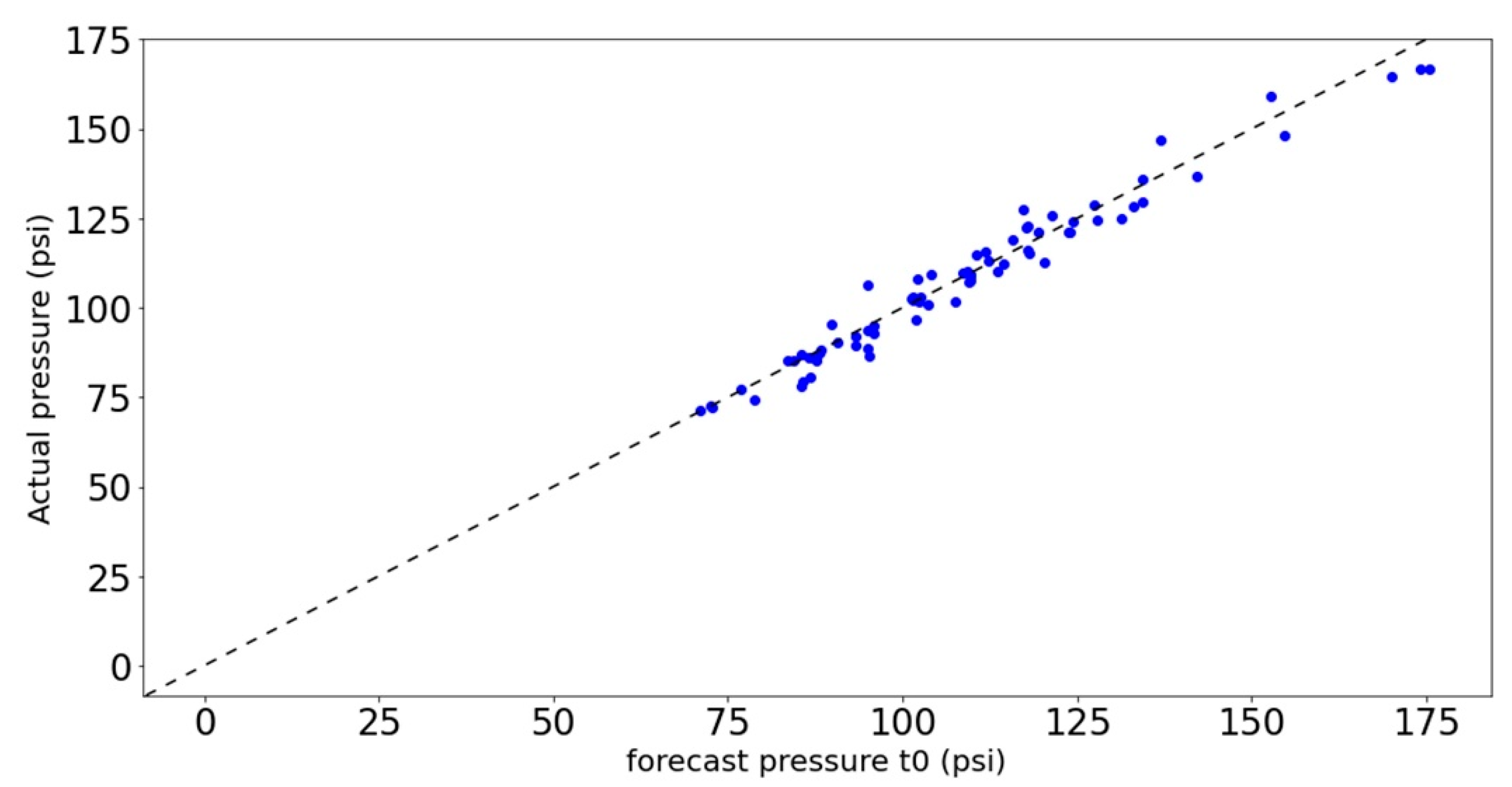
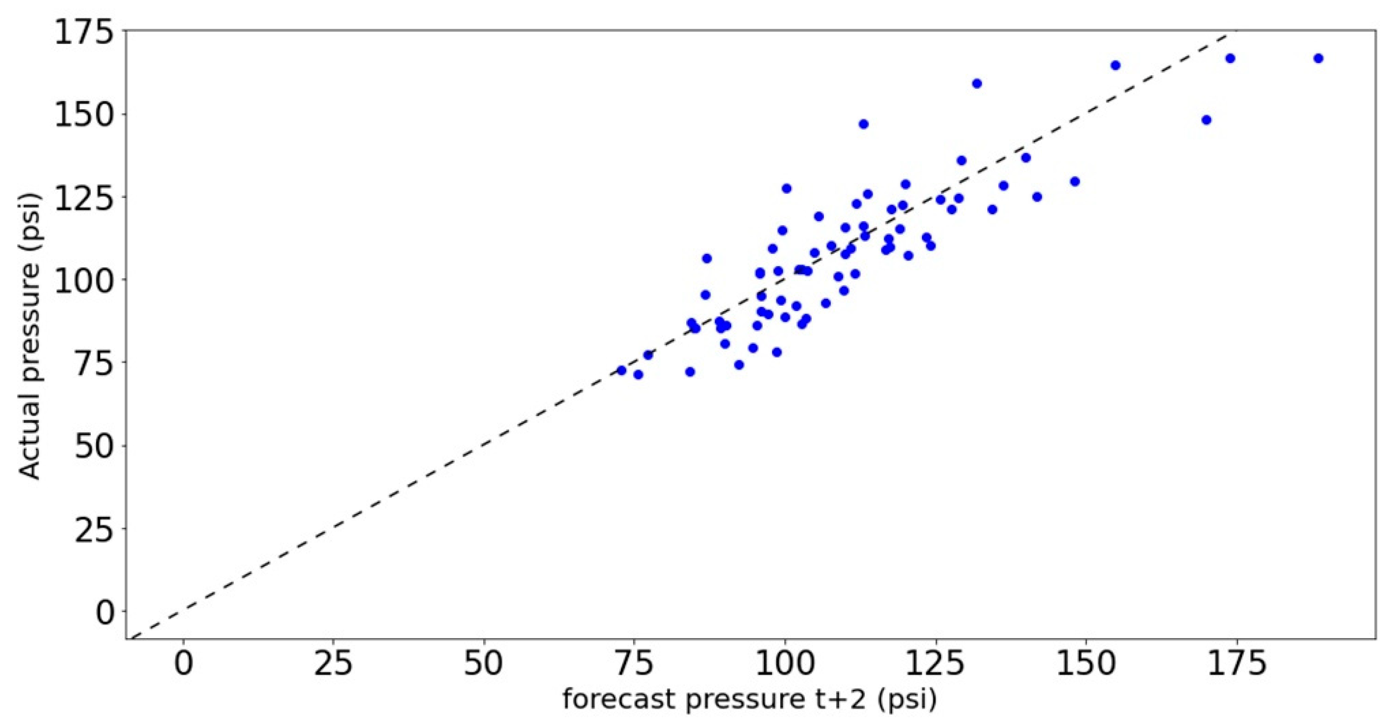
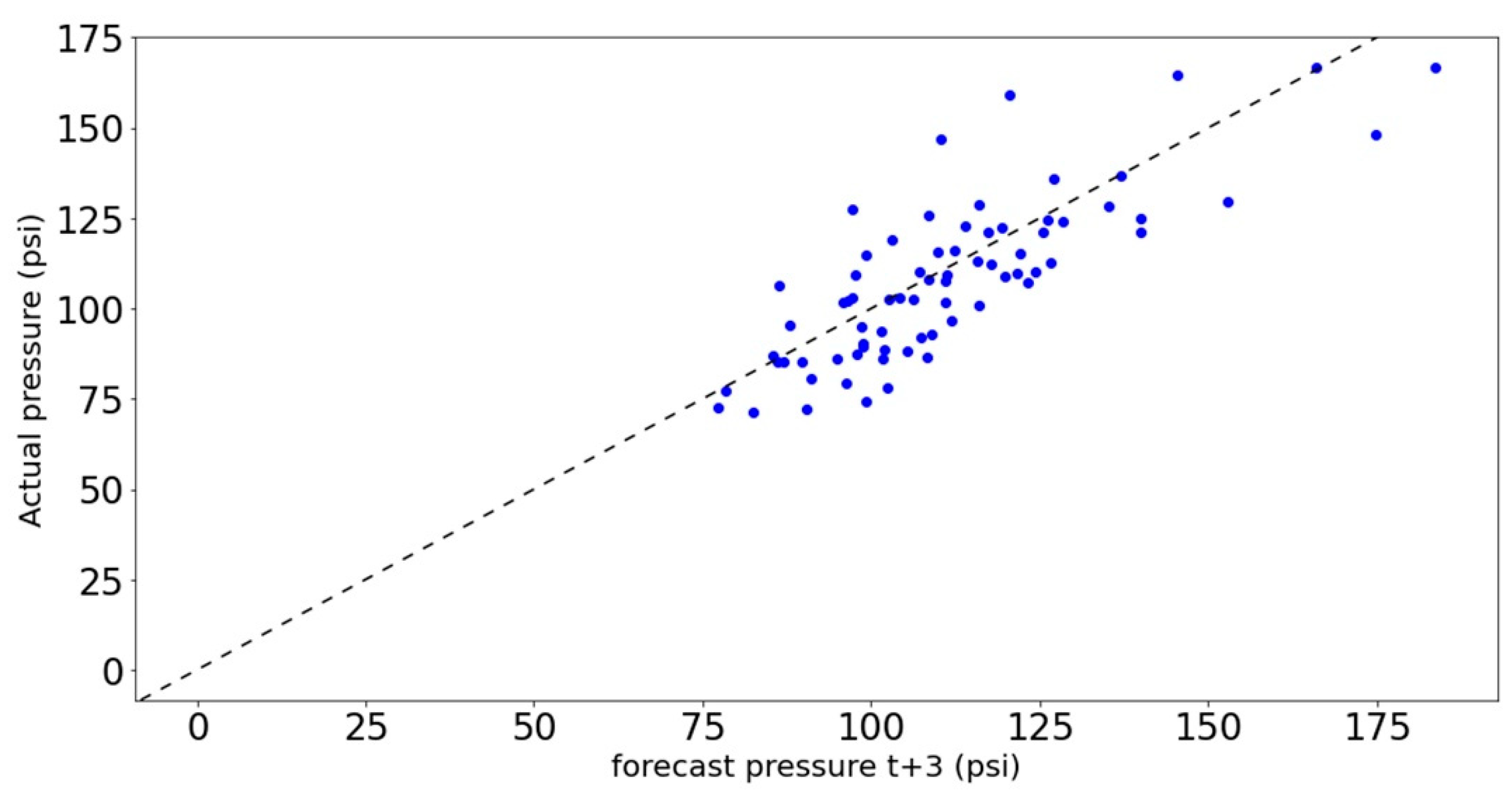
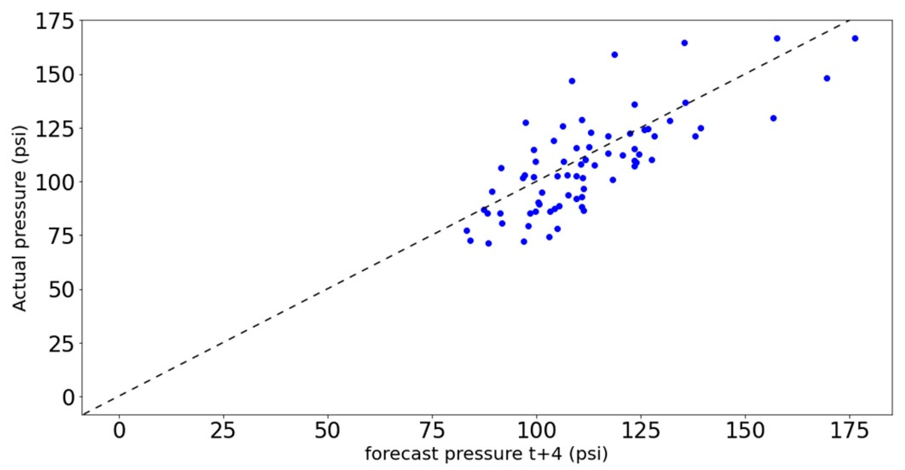
Table 3. RMSE and R2 evaluation for NARX-MLP.
StepRMSER2
t04.290.96
t + 16.830.89
t + 211.670.69
t + 313.440.59
t + 416.950.36
Publisher’s Note: MDPI stays neutral with regard to jurisdictional claims in published maps and institutional affiliations.

