Dynamic Measurements with the Bicone Interfacial Shear Rheometer: Numerical Bench-Marking of Flow Field-Based Data Processing

Abstract

Flow field-based methods are becoming increasingly popular for the analysis of interfacial shear rheology data. Such methods take properly into account the subphase drag by solving the Navier–Stokes equations for the bulk phase flows, together with the Boussinesq–Scriven boundary condition at the fluid–fluid interface and the probe equation of motion. Such methods have been successfully implemented on the double wall-ring (DWR), the magnetic rod (MR), and the bicone interfacial shear rheometers. However, a study of the errors introduced directly by the numerical processing is still lacking. Here, we report on a study of the errors introduced exclusively by the numerical procedure corresponding to the bicone geometry at an air–water interface. In our study, we set an input value of the complex interfacial viscosity, and we numerically obtained the corresponding flow field and the complex amplitude ratio for the probe motion. Then, we used the standard iterative procedure to obtain the calculated complex viscosity value. A detailed comparison of the set and calculated complex viscosity values was made in wide ranges of the three parameters herein used, namely the real and imaginary parts of the complex interfacial viscosity and the frequency. The observed discrepancies yield a detailed landscape of the numerically-introduced errors.

1. Introduction

Complex interfacial fluid systems have received much attention in recent years because of their interest from, both, a fundamental and applied point of view in living and industrial systems [1]. Systems such as tear film, the lung’s internal fluid film, cell membranes, foams, and emulsions constitute examples of complex interfacial fluid systems whose dynamical properties play a crucial role regarding their function or utility. Indeed, knowledge of the mechanical properties of such fluid interfacial systems is an essential factor in the development of medical therapies in lung [2] or eye diseases [3], or in the stability and performance of industrial products in the food [4], personal care [5,6], and oil recovery sectors [7].

The characterization of the rheology (mechanical properties) of complex interfacial fluid systems is a powerful tool to unravel the physico-chemical phenomena occurring in interfacial processes [1]. A full characterization of the mechanical properties of plane interfacial systems requires studying the mechanical response in two deformation modes [8,9,10], namely shear mode, which keeps the area constant while allowing for shape changes [9], and dilatational mode, which keeps the shape unchanged while allowing for area changes [10]. In this report, we will restrict ourselves to the shear deformation mode.

A very convenient way to characterize the dynamical viscoelasticity properties of complex fluid interfaces is through the low amplitude oscillatory motion of a probe located at the interface [11], which allows describing the interface rheology in terms of a complex interfacial dynamic modulus, $G_s^{*}\left(\omega \right)=G_s^{\prime }\left(\omega \right)+i{G}_s^{″}\left(\omega \right)$, where $G_s^{\prime }\left(\omega \right)$ accounts for the elastic component of the response and is called the interfacial storage modulus, and $G_s^{″}\left(\omega \right)$ represents the viscous component of the response and is called the interfacial loss modulus. Alternatively, a complex interfacial viscosity can be defined as ${\eta }_s^{*}\left(\omega \right)={\eta }_s^{\prime }\left(\omega \right)-i{\eta }_s^{″}\left(\omega \right)=i{G}_s^{*}\left(\omega \right)/\omega$, whose components are related to the interfacial dynamic moduli by ${\eta }_s^{\prime }=G_s^{″}/\omega$ and ${\eta }_s^{″}=G_s^{\prime }/\omega$.

Many experimental realizations of such oscillating probe techniques have been proposed, and as of today, three of them emerge as largely popular configurations for interfacial shear rheometers (ISR). Two of them are built around conventional rotational rheometers by using purposely-designed fixtures: a bicone bob [12] or a double wall-ring (DWR) [13]. The third configuration uses a magnetic rod probe whose oscillation is forced by either a suitably-driven Helmholtz coil pair [14] or a mobile magnetic tweezers actuator [15].

Under oscillatory forcing, the complex interfacial dynamic moduli (respectively, viscosity components) are obtained through the relationship between the amplitudes of the shear stress and the shear strain (respectively, rate) and their phase difference. In the rotational displacement configuration, shear stresses and strains (or rates) are directly related to the driving torque and the angular displacement. However, subtracting the effect of the subphase drag on the probe motion is, both, of paramount importance and highly non-trivial. An indication of the relative importance of the interface and subphase drags on the probe is given by the complex Boussinesq number, $B{o}^{*}$. For instance, in the case of an air/water interface, $B{o}^{*}$ is defined as [16]:

$$B{o}^{*}=\frac{{\eta }_s^{*}}{L\eta },$$

(1)

where ${\eta }_s^{*}$ is the complex interfacial viscosity, $\eta$ is the subphase bulk viscosity, and L is a characteristic length scale that depends on the geometric configuration of the rheometer.

The pioneering work in [17] opened the way to use computed flow fields in the interpretation of the interfacial rheology data. A further step forward was taken by introducing an iterative scheme to recover the value of the complex interfacial viscosity using the computationally-obtained flow field and the experimental values of the torque and angle amplitudes and relative phase in the DWR interfacial rheometer [13]. Since then, several flow field-based data processing schemes, adequate for the magnetic rod ISR [15,18,19] and the bicone ISR [20], have been proposed to take properly into account the subphase drag on the probe.

Such schemes share a common structure (see Figure 1), starting from a “seed” value of the complex interfacial viscosity, namely:

• Solve the Navier–Stokes equations for the subphase flow field with no slip boundary conditions at the container and probe walls and the Boussinesq–Scriven boundary condition at the interface.
• Use the obtained flow field to compute the subphase and interface drags on the probe.
• Use the probe equations of motion to obtain a new prediction for the value of the complex interfacial viscosity.
• Go back to Step 1 till convergence is obtained for the value of the complex interfacial viscosity.

Such schemes have rendered excellent results in the DWR [13], the magnetic rod ISRs, both in the Helmholtz coil [18] and the magnetic tweezers [15] configurations, and the bicone ISR [20], yielding good values of the complex interfacial viscosity and providing a more realistic separation of the real and imaginary parts of the complex interfacial viscosity. From a different perspective, fully-three-dimensional calculations of the flow field corresponding to the knife-edge interfacial shear rheometer in the case of purely-viscous interfaces have been shown to represent well the rheometer results both under continuous rotation [21] and oscillatory [22] modes.

From a practical point of view, an essential characteristic of each of the above-mentioned ISRs is their respective measuring range in a parameter space defined by ${\eta }_s^{\prime }$, ${\eta }_s^{″}$, and $\omega$. In this aspect, assessing the performance of the flow field based-iterative process is of paramount importance, particularly in the case of the bicone ISR, due to the comparatively higher role played by the subphase because of the larger subphase contact with the probe’s lower surface, which renders comparatively lower values of $B{o}^{*}$ [9]. Limited studies [20,23] of the available measuring range and the errors introduced by the iterative process have been made in the case of the bicone ISR. Knowledge of such errors and on the propagation of experimental errors through the data processing scheme are crucial to delimit the useful measuring range of the bicone ISR.

Here, we report on a more complete numerical bench-marking of the flow field-based data processing scheme when applied to the bicone ISR. This study has been made using a software package that we have recently made publicly available [24]. The software package uses an iterative scheme defined directly on $B{o}^{*}$ and makes extensive use of the sparse matrix functions in MATLAB.

To that purpose, we have defined two numerical problems, a direct one (given ${\eta }_s^{\prime }$, ${\eta }_s^{″}$, and $\omega$, find the complex amplitude ratio, $A{R}^{*}$) and an inverse one (given $A{R}^{*}$ and $\omega$ find ${\eta }_s^{\prime }$ and ${\eta }_s^{″}$ through the iterative process). The software has been slightly modified so that the the flow field obtained with the “seed” ${\eta }_s^{\prime }$ and ${\eta }_s^{″}$ values is used to obtain the complex amplitude ratio, which is the solution of the direct problem.

Using the output of the direct problem as the input of the inverse one, we have made a detailed study of the consistency of the iterative data processing scheme in terms of the differences appearing between the complex viscosity input values of the direct problem and the corresponding output values of the inverse problem. Further imposing the requirement that the complex amplitude ratio must be different from the one corresponding to a clean water interface allows us to draw a complete map of the parameter space available to the bicone ISR when using the flow field-based data processing scheme. Finally, we show the results of a numerical study of the propagation of the experimental uncertainties in the modulus and the argument of the complex amplitude ratio through the data processing scheme.

2. Hydrodynamic Model and Data Analysis Scheme

The hydrodynamic model and data analysis scheme have been fully described elsewhere [23]. We reproduce it here just for the sake of completeness. The geometrical configuration for an air/water interface is depicted in Figure 2. The system is made from a cylindrical cup of radius $R_c$, which is at rest, and a conical bob fixture, with radius $R_b$, attached to the axis of a rotational rheometer. The subphase is the bulk fluid phase located below the interface, and it is in mechanical contact with the conical surface of the bob.

The interface is considered flat and horizontal, and the flow, both at the subphase and the interfaces, is considered horizontal and axially symmetric. The angular oscillation of the bicone is considered periodic, with frequency $\omega$. Hence, the bicone angular oscillation and the velocity at the bicone rim can be written as:

$$\theta \left(t\right)={\theta }_0{e}^{i\omega t};v_{\theta }(R_b,h,t)=i{R}_b\omega {\theta }_0{e}^{i\omega t}.$$

Under such approximations, the spatial dependence of the fluid velocity field can be represented by a complex amplitude function $g^{*}(r,z)$ so that:

$$v_{\theta }(r,z,t)=i{R}_b\omega g^{*}(r,z){\theta }_0{e}^{i\omega t},$$

(2)

where the spatial variables have been made non-dimensional taking $R_b$ as the characteristic length scale. The complex amplitude function must obey Equation (3), derived from the Navier–Stokes equations, which in non-dimensional form reads:

$$iR{e}^{*}{g}^{*}(\overline{r},\overline{z})=\frac{{\partial }^2{g}^{*}(\overline{r},\overline{z})}{\partial {\overline{r}}^2}+\frac{{\partial }^2{g}^{*}(\overline{r},\overline{z})}{\partial {\overline{z}}^2}+\frac{1}{\overline{r}}\frac{\partial g^{*}(\overline{r},\overline{z})}{\partial \overline{r}}-\frac{g^{*}(\overline{r},\overline{z})}{{\overline{r}}^2},$$

(3)

where $R{e}^{*}$ is the Reynolds number, $R{e}^{*}=\rho \omega R_c^2/{\eta }^{*}$ (possibly complex if the bulk subphase viscosity is complex). The boundary conditions are no-slip at the cup and bicone bob walls (Equation (4)), and the Boussinesq–Scriven boundary conditions (tangential stress balance) at the interface (Equation (5)) are:

$$\begin{array}{c}{g}^{*}(\overline{r},0)=g^{*}(1,\overline{z})=0,\hfill \\ g^{*}(0,\overline{z})=0,\hfill \\ g^{*}(\overline{r}\le {\overline{R}}_b,\overline{h})=\frac{\overline{r}}{{\overline{R}}_b},\hfill \end{array}$$

(4)

$$\frac{\partial g^{*}}{\partial \overline{z}}=B{o}^{*}\frac{\partial }{\partial \overline{r}}\left(\frac{1}{\overline{r}}\frac{\partial }{\partial \overline{r}}\left(\overline{r}{g}^{*}\right)\right),\mathrm{at}{\overline{R}}_b<\overline{r}<1,\overline{z}=\overline{h},$$

(5)

where $B{o}^{*}={\eta }_s^{*}/R_c{\eta }^{*}$.

The torque balance equation for the ISR rotor yields Equation (6), which relates the complex amplitude ratio to, both, the Boussinesq number and, implicitly, the velocity amplitude function $g^{*}(\overline{r},\overline{z})$:

$$A{R}^{*}=i\omega 2\pi R_b{\eta }^{*}\left[{\int }_0^{R_b}{r}^2\left(\frac{\partial g^{*}}{\partial z}\right){|}_{z=h}dr-R_b{R}_{c}B{o}^{*}\left(R_b\left(\frac{\partial g^{*}}{\partial r}\right){|}_{r=R_b,z=h}-1\right)\right]-I{\omega }^2.$$

(6)

Solving for the Boussinesq number allows one to setup a simple iterative procedure, namely,

$$B{o}^{*\{i+1\}}=\frac{-A{R}_{exp}^{*}-I{\omega }^2+i\omega 2\pi R_b{\eta }^{*}{\int }_0^{R_b}{r}^2{\left.\left(\frac{\partial g^{*\left\{i\right\}}}{\partial z}\right)\right|}_{z=h}dr}{i\omega 2\pi {\eta }^{*}{R}_b^2{R}_c\left(R_b{\left.\left(\frac{\partial g^{*\left\{i\right\}}}{\partial r}\right)\right|}_{r=R_b,z=h}-1\right)},$$

(7)

where $A{R}_{exp}^{*}$ represents the complex value of the experimentally-obtained amplitude ratio. As the value of $A{R}_{exp}^{*}$ comes directly from the experiments, it seems adequate to establish the convergence upon the complex amplitude ratio as:

$$\left|\frac{{\left(A{R}_{pp}^{*}\right)}_{calc}^{\left\{i\right\}}-{\left(A{R}_{pp}^{*}\right)}_{exp}}{{\left(A{R}_{pp}^{*}\right)}_{exp}}\right|\le tolMin.$$

(8)

3. Results

In this section, we show the results obtained through extensive numerical calculations aiming at evaluating the performance of the iterative data processing scheme when applied to a bicone interfacial rheometer working in oscillatory mode at an air/water interface.

A careful evaluation of the dependence on the mesh size of the spatial velocity gradients’ representation, the number of iterations needed for convergence, and the computational costs of the procedure was reported in [23], where preliminary explorations of the consistency of the iterative data processing scheme, by sweeping in the complex interfacial viscosity while keeping $\omega$ constant, were also included.

Here, at variance with respect to [23], we will focus, first, on checking the consistency of the iterative processing scheme upon changes of the oscillation frequency in the typical range explored in real experiments and, second, on analyzing the measuring range achievable with a bicone ISR when using the proposed flow field-based data analysis scheme. This last aspect will be illustrated through the analysis of the achievable measuring range of a bicone fixture in our Bohlin C-VOR rheometer.

3.1. Consistency of the Iterative Data Analysis Scheme

3.1.1. Consistency over the Frequency Range

We say the iterative procedure is consistent if working on input data ($A{R}^{*}$ values) corresponding to known values of ${\eta }^{*}$ yields output values of the interfacial viscosity that are very close to the known ones. We studied the consistency of the iterative data analysis scheme through the following general procedure: (i) preset the frequency, $\omega$, and the complex interfacial viscosity, ${{\eta }_s^{*}}_{prog}$, and solve the direct problem that yields the corresponding complex amplitude ratio $A{R}_{prog}^{*}$, and (ii) use the obtained value of the complex amplitude ratio as the input of the inverse problem, and obtain the calculated value of the complex interfacial viscosity, ${{\eta }_s^{*}}_{calc}$. The relative difference between the preset and calculated values of ${\eta }_s^{*}$ will give us an idea of the consistency of the numerical scheme.

In Figure 3, we show the results of such a procedure for a frequency sweep in the range $0.06\le \omega \le 62.83$ rad/s. Representative values of the complex interfacial viscosity have been chosen, namely a purely-viscous interface (${\eta }_s^{*}={\eta }_s^{\prime }$, i.e., ${\eta }_s^{″}=0$), a viscoelastic interface (${\eta }_s^{*}={\eta }_s^{\prime }-i{\eta }_s^{″}$, where ${\eta }_s^{\prime }={\eta }_s^{″}$), and a purely-elastic interface (${\eta }_s^{*}=-i{\eta }_s^{\prime }$, i.e., ${\eta }^{\prime }=0$). Three typical numerical values of ${\eta }_s$ have been used in the above-described cases: ${\eta }_s={10}^{-6},{\eta }_s={10}^{-4},{\eta }_s={10}^{-2}$, in units of N s/m.

The graphs in the left column illustrate the results obtained for ${{\eta }_s^{\prime }}_{calc}$ and ${{\eta }_s^{″}}_{calc}$ as a function of frequency, while the right column holds the graphs of the number of iterations needed for convergence at each frequency. The graphs in the upper row (Graphs (a) and (b)) pertain to the purely-viscous interface, those in the middle row (Graphs (c) and (d)) to the viscoelastic interface, and the lower row graphs ((e) and (f)) the data corresponding to the purely-elastic interface. In the left column graphs, filled and empty circles are used to represent the values of ${{\eta }_s^{\prime }}_{calc}$ and ${{\eta }_s^{″}}_{calc}$, respectively. Symbols’ colors of black, red, and blue correspond, respectively, to the high, middle, and low numerical values of ${\eta }_s$ mentioned above.

The agreement between the obtained viscosity component values and the non-null programmed values was remarkable (in the case of the viscoelastic interface, solid and empty circles superpose, as expected). However, unavoidable numerical errors and the finite convergence tolerance, given by the $tolMin$ parameter (Equation (8)), necessarily give rise to non-null values of ${{\eta }_s^{″}}_{calc}$ for the purely-viscous interface (Graphs (a) and (b)) and ${{\eta }_s^{\prime }}_{calc}$ for the purely-elastic interface (Graphs (e) and (f)). Fortunately, these pathological non-null values were in all of the cases herein studied more than two orders of magnitude below their measurable counterparts (${{\eta }_s^{\prime }}_{calc}$ for the purely-viscous interface and ${{\eta }_s^{″}}_{calc}$ for the purely-elastic interface).

The graphs in the right column show that in the studied frequency range, convergence in the inverse problem always occurred in less than 25 iterations. Particularly remarkable is the case with the higher complex viscosity modulus (${\eta }_s={10}^{-2}$ N s/m, black symbols), where convergence occurred in three iterations for the whole frequency range. Interestingly, for intermediate values of the complex viscosity modulus (red symbols), increasing the frequency had a destabilizing effect (more iterations were required for convergence), while for a very low complex viscosity modulus (blue symbols), the effect was just the opposite (less iterations were needed for convergence upon increasing the frequency).

The visual agreement between the obtained viscosity component values and the non-null programmed values in the graphs in the left column of Figure 3 can be better ascertained calculating the relative difference between the programmed and calculated values and representing it in a logarithmic vertical scale. Figure 4 shows such graphs, where row arrangement and symbols’ shapes and colors maintain the same codding as in Figure 3. To be specific, the relative differences have been calculated as:

$${\delta }_{{\eta }^{\prime }}=100\times \left|\frac{{{\eta }_s^{\prime }}_{calc}-{{\eta }_s^{\prime }}_{prog}}{{{\eta }_s^{\prime }}_{prog}}\right|;{\delta }_{{\eta }^{″}}=100\times \left|\frac{{{\eta }_s^{″}}_{calc}-{{\eta }_s^{″}}_{prog}}{{{\eta }_s^{″}}_{prog}}\right|$$

Several common features appear in the three graphs included in Figure 4. First, the relative differences were overall increasing functions of frequency, although non-monotonic in some cases. Second, the relative differences were higher the smaller the value of ${\eta }_s^{\prime }$ or ${\eta }_s^{″}$. Nonetheless, such relative differences were of the order of a few percent in the worst case —lowest numerical value of ${\eta }_s^{\prime }$ or ${\eta }_s^{″}$ and highest frequency value— and smaller in all of the other cases. In the case of the viscoelastic interface, the relative differences were very similar in, both, the real and imaginary parts of the complex viscosity. The physical origin of the general increasing tendency with frequency of the relative errors shown in Figure 4 is not clear to us. One might guess that rotor inertia might be at play at high frequency values, but then, an ${\omega }^2$ tendency should be expected, which is not the case.

3.1.2. Consistency in the Complex Plane

A complementary view of the consistency problem can be drawn through the percentage modulus of the complex relative differences between ${{\eta }_s^{*}}_{calc}$ and ${{\eta }_s^{*}}_{prog}$, i.e.,

$${\delta }_{mod}=100\times \left|\frac{{{\eta }_s^{*}}_{prog}-{{\eta }_s^{*}}_{calc}}{{{\eta }_s^{*}}_{prog}}\right|$$

We have calculated the values of ${\delta }_{mod}$ at $60\times 60$ logarithmically-spaced points in the $({\eta }_s^{\prime },{\eta }_s^{″})$ plane, in the range ${10}^{-6}\le {\eta }_s^{\prime },{\eta }_s^{″}\le {10}^{-3}$ in units of N s/m, at three representative frequency values, namely, 0.63, 6.28, and 62.83 rad/s. The values so obtained have been used to construct contour plots of ${\delta }_{mod}$ in the $({\eta }_s^{\prime },{\eta }_s^{″})$ plane, which are shown in Figure 5.

The contour lines correspond to the following percentage values of ${\delta }_{mod}$: (a) 0.01, 0.02, 0.04, 0.1; (b) 0.15, 0.3, 1, 30; (c) 0.2, 0.5, 1, 2. In the three graphs, red dashed lines correspond to the highest ${\delta }_{mod}$ value and continuous light blue lines to the lowest ${\delta }_{mod}$ value. Hence, the interpretation of the contour lines is that, taking as an example the light blue line in Figure 5, at the region to the left and below that light blue line, the value of ${{\eta }_s^{*}}_{calc}$ differs from the value of ${{\eta }_s^{*}}_{prog}$ by more than $0.2\%$

The aspect of the contour lines was not smooth, with even the appearance of some islands. However, it might be possible that such islands were an artifact caused by the limited resolution of only $60\times 60$ points in the $({\eta }_s^{\prime },{\eta }_s^{″})$ plane, due to the high computational cost of these simulations.

However, some general observations can be made of Figure 5. In the three cases herein considered, the structure of the contour lines corresponding to the lower values of ${\delta }_{mod}$ (continuous light blue lines) roughly formed a square with the coordinate axes. Strong peaks (red dashed lines) appeared close to low values of ${\eta }_s^{\prime }$ (close to the ordinate axis), i.e., in elasticity-dominated interfaces. No such peaks appeared close to low values of ${\eta }_s^{″}$ (close to the abscissa axis), i.e., in viscosity-dominated interfaces.

Regarding the performance of the iterative data processing scheme, it is important to look at the numerical values of ${\delta }_{mod}$ in each of the graphs having in mind that it represents the modulus of the relative difference between two values of the complex interfacial viscosity: the programmed value at the start of the direct problem and the calculated value at the end of the inverse problem.

In Graph (a), ${\delta }_{mod}$ takes very low values. all of them being lower than $0.2\%$, while ${\delta }_{mod}\le 0.1\%$ in the region such that ${\eta }_s^{\prime }\ge 2\times {10}^{-6}$ and ${\eta }_s^{″}\ge {10}^{-5}$ in units of N m/s. This means that the iterative process introduced very small errors ($\le 0.1\%$) in the interfacial viscosity measurements within most of the $({\eta }_s^{\prime },{\eta }_s^{″})$ range herein considered, provided they were made at low oscillation frequencies (0.63 rad/s in the top graph).

In Graph (b) of Figure 5, the values of ${\delta }_{mod}$ are much higher (up to $60\%$ at the peak), while ${\delta }_{mod}\le 0.15\%$ in the region such that ${\eta }_s^{\prime }\ge {10}^{-5}$ and ${\eta }_s^{″}\ge 3\times {10}^{-5}$. Hence, the $({\eta }_s^{\prime },{\eta }_s^{″})$ range in which the iterative process introduces small errors decreased significantly at an oscillation frequency of $6.28$ rad/s.

This tendency is again clear in Graph (c) of Figure 5. Although the values of ${\delta }_{mod}$ were lower than in the previous case (about $2.5\%$ at the peak), the low error region (${\delta }_{mod}\le 0.2\%$) shrank again to values such that ${\eta }_s^{\prime }\ge {10}^{-4}$ and ${\eta }_s^{″}\ge {10}^{-4}$ in units of N m/s.

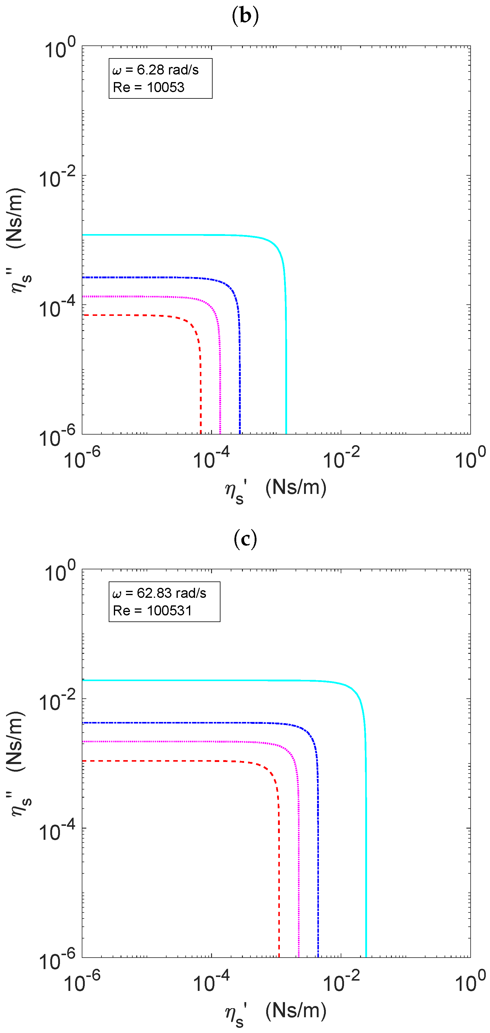
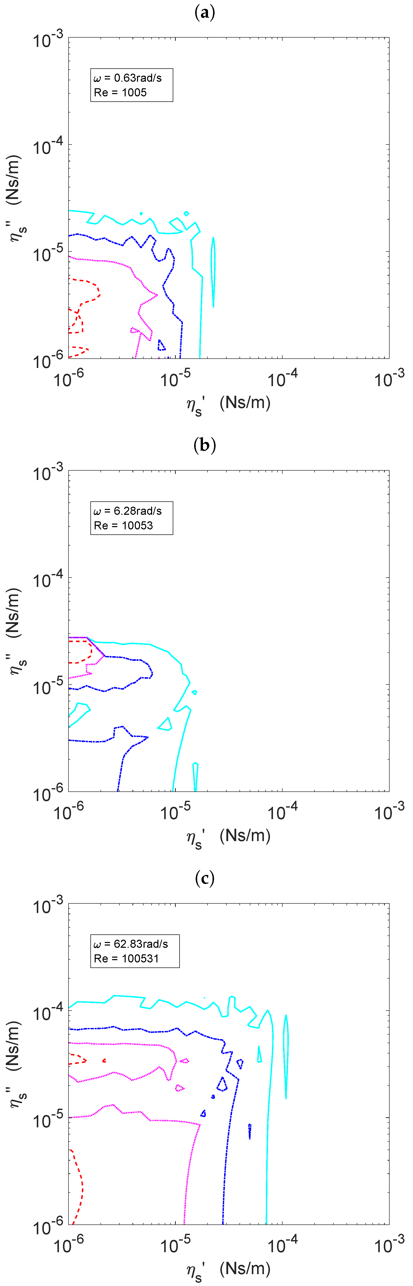
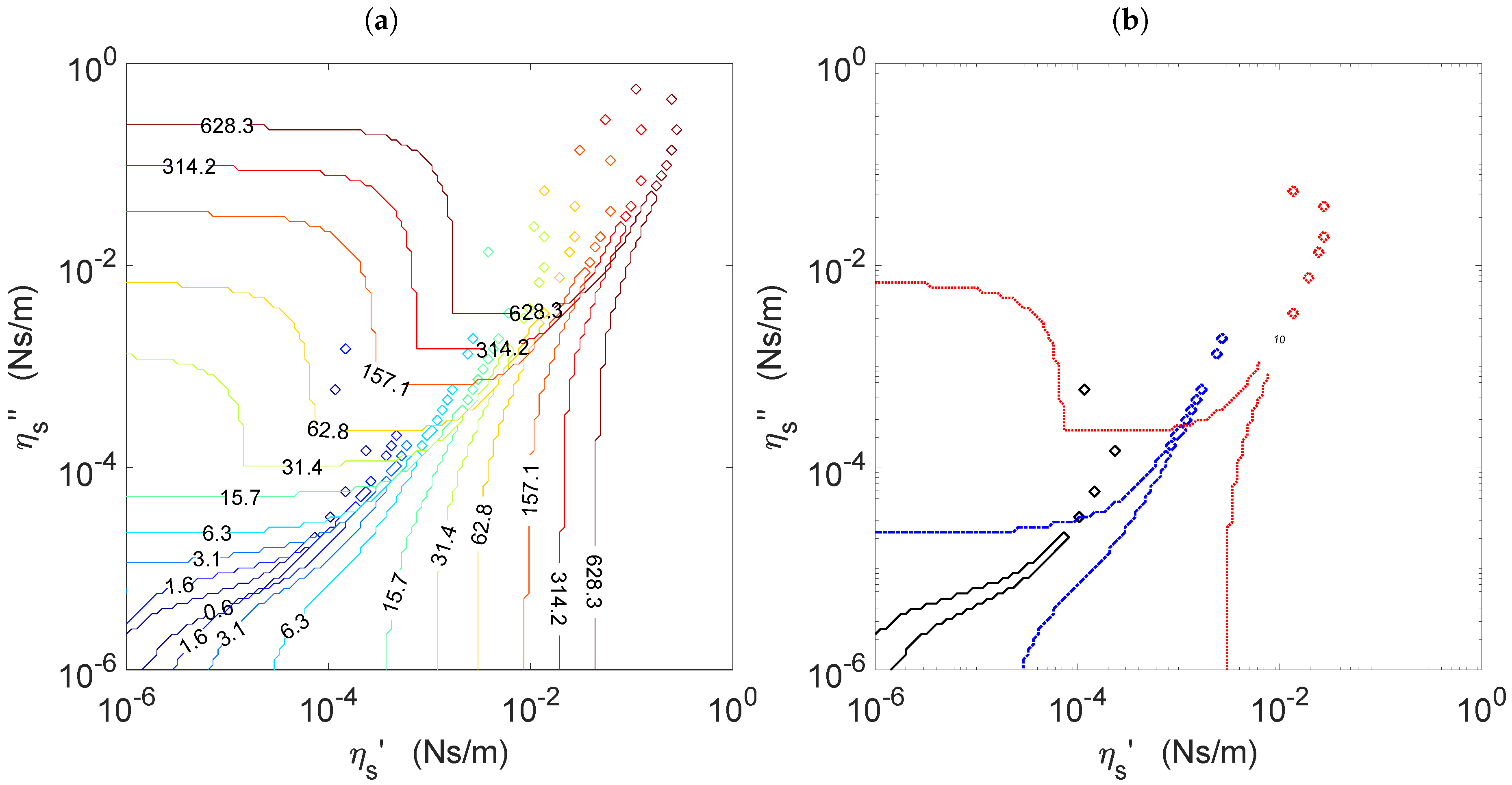
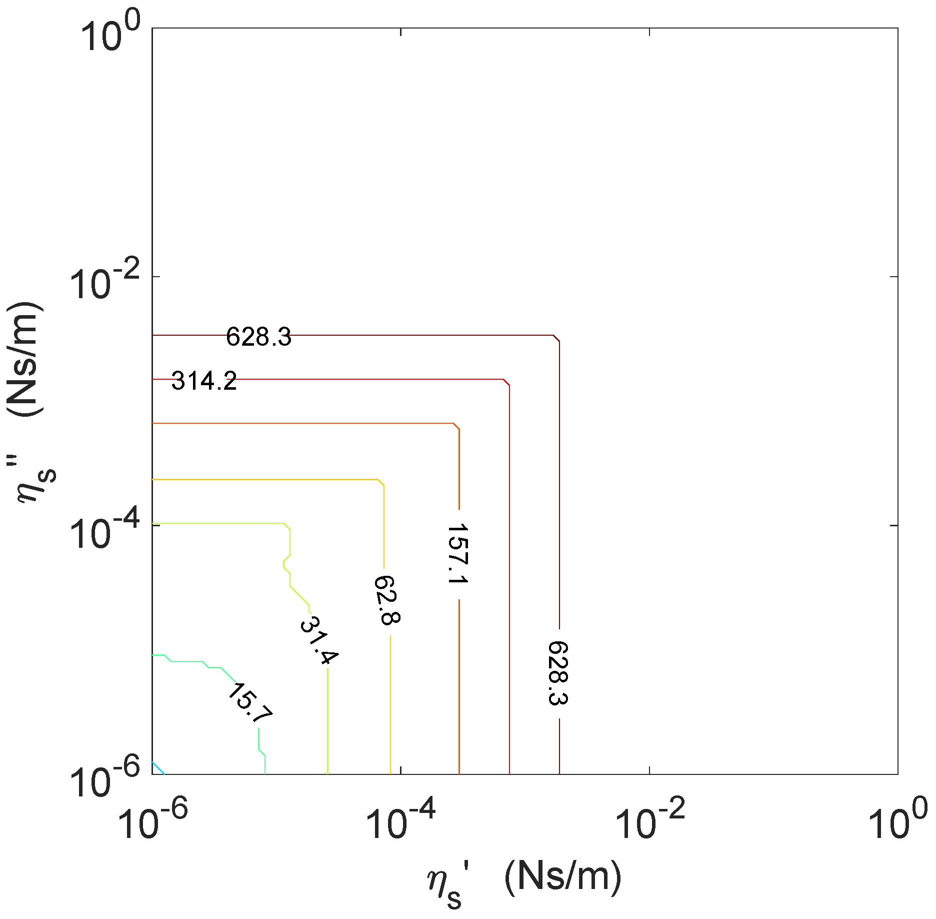
3.2. Estimation of the Achievable Measuring Range

To elucidate which is the achievable measuring range of a bicone ISR when using the proposed flow field-based data analysis scheme, two main aspects have to be considered: on the one hand, the instrumental errors, i.e., the unavoidable dispersion in the torque and angular displacement data measured by the rheometer; on the other hand, the rheometry point of view, i.e., the fact that for the measurements to be acceptable, they must be distinguishable from those pertaining to a clean water interface. The interplay between these two aspects is illustrated here through the analysis of the achievable measuring range of a bicone fixture in a Bohlin C-VOR rheometer.

In oscillatory measurements, the output of the rheometer comprises the amplitudes of the torque and the angular displacement and their relative phase, which are used to determine the experimental value of the amplitude ratio, $A{R}_{exp}^{*}$. Given a surfactant laden interface, the instrument can resolve its complex viscosity if the corresponding complex amplitude ratio can be distinguished from that pertaining to a clean water interface. In [20], this condition was formally expressed as two inequalities that, both, had to be fulfilled simultaneously.

$$\left|\left|A{R}_{exp}^{*}\right|-\left|A{R}_{clean}^{*}\right|\right|\ge \sigma \left(\left|A{R}^{*}clean\right|\right);\left|arg\left(A{R}_{exp}^{*}\right)-arg\left(A{R}_{clean}^{*}\right)\right|\ge \sigma \left(arg\left(A{R}_{clean}^{*}\right)\right).$$

(9)

In order to apply Equation (9), we have calculated both $A{R}_{exp}^{*}$ and $A{R}_{clean}^{*}$ for different ${\eta }_s^{\prime },{\eta }_s^{″}$ combinations. At variance with respect to [20], where only a few combinations of ${\eta }_s^{\prime },{\eta }_s^{″}$ values were investigated, here, a thorough exploration of the $({\eta }_s^{\prime },{\eta }_s^{″})$ has been performed by using all the combinations of 120 values logarithmically spaced in each axis and different frequencies. The corresponding values for the uncertainties $\sigma \left(\left|A{R}_{clean}^{*}\right|\right)$ and $\sigma (arg\left(A{R}_{clean}^{*}\right)$ were taken from experiments performed on clean water interfaces of the Bohlin C-VOR rheometer.

In Figure 6a, we show the lines satisfying the equality in Equation (9), i.e., the lower resolvable limit, for frequencies in the range $0.63\le \omega \le 628.32$ rad/s. For a clearer view, the lines corresponding to three representative frequencies, namely, $\omega =0.63$, $6.28$, and $62.83$ rad/s, are shown in Figure 6b.

The structure of the non-measurable region had some common features at all frequencies, such as the spiky tongue that widened at lower values of the real and imaginary parts of the viscosity. The island-like structures at the tips of the tongues were artifacts caused by the width of the tongue being comparable to the distance between sampled points in the $({\eta }_s^{\prime },{\eta }_s^{″})$ plane. In fact, such islands should actually correspond to points corresponding to a continuous tongue that is getting thinner and thinner. The tongues shift to cover larger values of ${\eta }_s^{\prime }$ and ${\eta }_s^{″}$ as the frequency increases.

For viscosity-dominated interfaces (very low ${\eta }_s^{″}$), there was, at each frequency, a well-defined threshold interfacial viscosity, below which the interface was non-distinguishable from a clean water interface. Roughly speaking, those thresholds were (in N s/m units) $2\times {10}^{-6}$ for $\omega =0.63$ rad/s, $3\times {10}^{-5}$ for $\omega =6.28$ rad/s, and $3\times {10}^{-3}$ for $\omega =62.83$ rad/s. A similar behavior was illustrated in Figure 7.c of [20], although there, sweeping was done only in ${{\eta }^{\prime }}_s$.

A different behavior was seen for viscoelastic interfaces. Let us consider viscoelastic interfaces with ${\eta }_s^{\prime }={\eta }_s^{″}$ (points at the bisectrix of Figure 6, either (a) or (b)). For low values of ${\eta }_s$, the points lied in the base of the tongue, and therefore, the interface was non-distinguishable from a clean water one. Increasing in ${\eta }_s^{\prime }={\eta }_s^{″}$, the tongue crossed below the bisectrix, and therefore, the points at the bisectrix became distinguishable from clean water interfaces. Upon further increasing ${\eta }_s^{\prime }={\eta }_s^{″}$, the tongue turned up and crossed again the bisectrix in a region in which the tongue was already very narrow. Hence, a very narrow window appeared in which the interface was again non-distinguishable from a clean water one. For ${\eta }_s^{\prime }={\eta }_s^{″}$ values larger than those at the above-mentioned window, the interface was again distinguishable from clean water. A similar behavior was illustrated in Figure 7.b of [20], although there, sweeping was made only along the bisector of the plane (${{\eta }^{\prime }}_s={\eta }_s^{″}$).

For elasticity-dominated interfaces (${\eta }_s^{″}\gg {\eta }_s^{\prime }$), one finds (see the lines corresponding to $\omega =0.63$ and $6.28$ rad/s) that at low values of ${\eta }_s^{″}$, the interface was not distinguishable from a clean water one, and there was, at each frequency, a well-defined threshold interfacial elastic component (${\eta }_s^{″}$) below which the interface was non-distinguishable from a clean water interface. Above the threshold value, the interfacial viscoelasticity can be measured. This scenario was similar to the one illustrated in Figure 4c,e of the Supporting Information of [20], made by sweeping only in ${\eta }_s^{\prime }$, except that in those figures, narrow tongues appeared, in which the interface was again non-distinguishable from a clean water one. This means that the sampling of the (${\eta }_s^{\prime },{\eta }_s^{″}$) plane in Figure 6 is not enough to represent the narrow parts of the tongues fully.

All of the above-mentioned features came from the non-fulfillment of the condition on the moduli. At large frequencies, however, the non-fulfillment of the condition on the arguments in Equation (9) caused an additional enlargement of the non-distinguishable region in elasticity-dominated interfaces. For instance, the line corresponding to $\omega =62.83$ rad/s in Figure 6b shows a bump at high values of ${\eta }_s^{″}$ and comparatively lower values of ${\eta }_s^{\prime }$. Actually, in our numerical simulations, that bump appeared at all frequency values above $15.7$ rad/s and shifted upwards and rightwards upon increasing the frequency (see Figure 6a). Indeed, as from our simulations, it cannot be discarded that for lower frequencies, similar bumps appeared as well at values ${\eta }_s^{\prime }<{10}^{-6}$ N s/m.

The distinguishability criterion based on simultaneous fulfillment of the two inequalities in Equation (9) was, however, somewhat too strict. In fact, when any of the two inequalities was fulfilled, the interface was already distinguishable from the clean water interface. If we use this relaxed criterion with the output of our simulations, the picture so obtained is as shown in Figure 7, where both the resonance tongues, due to the condition on the moduli, and the bumps at the elasticity dominated region, due to the condition on the arguments, have disappeared.

The distinguishability criterion based on simultaneous fulfillment of the two inequalities in Equation (9) was, however, somewhat too strict. In principle, when any of the two inequalities was fulfilled, the interface was already distinguishable from the clean water interface. If we impose this relaxed criterion on the output of our simulations, we obtain the picture shown in Figure 7. Some features are noticeable here. Generally speaking, the non-distinguishable region takes now a rectangular form, and the boundaries in ${\eta }_s^{\prime }$ and ${\eta }_s^{″}$ at each frequency have shifted to lower values. Two other main effects can be observed. Both the resonance tongues, for viscoelastic interfaces, and the bumps, for mainly elastic interfaces, disappeared. For frequencies smaller than those present in the labels of the contour lines in Figure 7, the boundaries of the non-distinguishable regions lied below the lower limits of the axis shown in the figure.

The resonance tongues are regions in which the inequality concerning the arguments is fulfilled while the one involving the moduli of the amplitude ratio is not. The bumps are just the opposite, namely regions in which the inequality concerning the moduli of the amplitude ratio is fulfilled while the one involving the argument is not.

From the experimental point of view, two important consequences can be derived from the differences between Figure 6 and Figure 7. For purely-viscous interfaces (very low ${\eta }_s^{″}$), the differences between Figure 6 and Figure 7 indicate that, in an experiment increasing ${\eta }_s^{\prime }$ from negligible values, one should expect going through three stages: from a low viscosity region, in which none of the inequalities will be fulfilled, to a second region, in which the argument inequality will be fulfilled, but not the amplitude’s, to a third regime, in which both inequalities will be fulfilled. In other words, for mainly viscous interfaces, the increase of viscosity should be perceived first as an increase in the argument of the amplitude ratio, and not as a decrease of the modulus of the amplitude ratio.

Conversely, for purely-elastic interfaces (very low ${\eta }_s^{\prime }$), the differences between Figure 6 and Figure 7 indicate that, in an experiment increasing ${\eta }_s^{″}$ from negligible values, the results obtained will go through three stages: from a low elasticity region, in which none of the inequalities will be fulfilled, to a second region, in which the inequality involving the moduli will be fulfilled, but not the one involving the arguments, to a third regime, in which both inequalities will be fulfilled. In other words, for mainly elastic interfaces, the increase of elasticity should be perceived first as a decrease in the modulus of the amplitude ratio, and not as an increase of the argument.

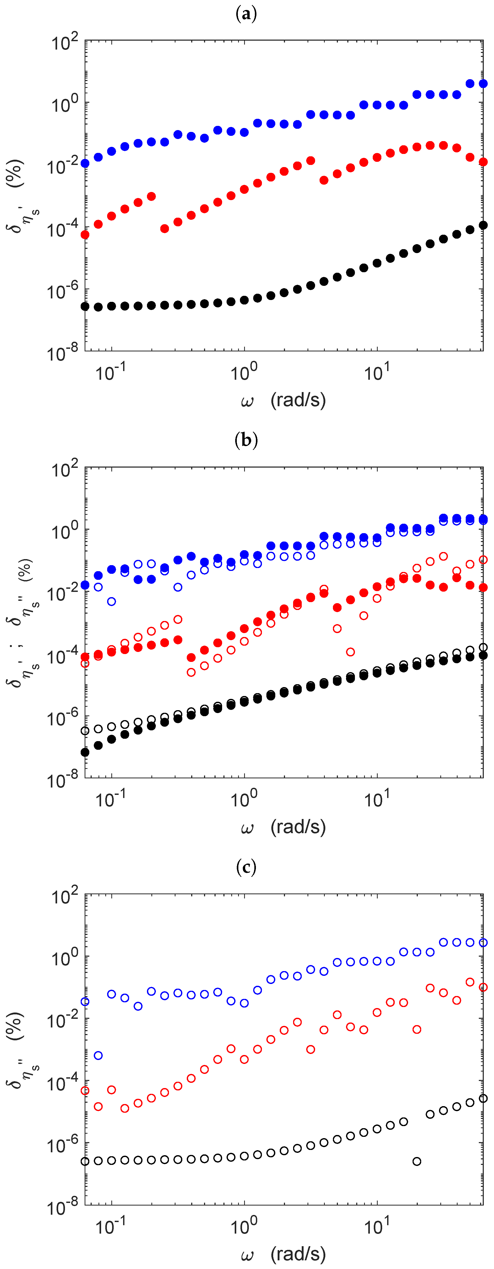
3.3. Global Relative Errors

In the previous subsections, we illustrated separately the errors introduced by the iterative process and the regions where the interface can be distinguished from a clean water one. However, in actual experiments, these two effects are coupled, because what one has as the result of an experiment is the values of the modulus and argument of the complex amplitude ratio, $\left|A{R}_{exp}^{*}\right|$ and ${\delta }_{exp}=arg\left(A{R}_{exp}^{*}\right)$, each one of which is then affected by its own experimental uncertainty, $\sigma \left(\left|A{R}_{exp}^{*}\right|\right)$ and $\sigma \left(arg\left(A{R}_{exp}^{*}\right)\right)$. Therefore, the problem here is how the small area around the experimental values defined by the rectangle defined by the points $\left(\left|A{R}_{exp}^{*}\right|\pm \sigma \left(\left|A{R}_{exp}^{*}\right|\right),{\delta }_{exp}\pm \sigma \left(arg\left(A{R}_{exp}^{*}\right)\right)\right)$ transforms under the application of the iterative procedure, i.e., how the uncertainties in the modulus and the argument of the amplitude ratio obtained experimentally propagate through the iterative data processing scheme.

In order to estimate that transformation, we programmed $60\times 60$ ${{\eta }_s^{\prime }}_{prog}$ and ${{\eta }_s^{″}}_{prog}$ values in a logarithmic mesh in $\left({{\eta }_s^{\prime }}_{prog},{{\eta }_s^{″}}_{prog}\right)$, and used them as input values for the direct problem, having as output the values of $\left|A{R}_{prog}^{*}\right|$ and ${\delta }_{prog}$. For each of those data, we used as uncertainty the experimental uncertainty measured for a clean water interface at the corresponding frequency and defined an enclosing rectangle with the points $\left(\left|A{R}_{prog}^{*}\right|\pm \sigma \left(\left|A{R}_{clean}^{*}\right|\right),{\delta }_{prog}\pm \sigma \left(arg\left(A{R}_{clean}^{*}\right)\right)\right)$. Next, we used the corners of such a rectangle plus the middle points of the four rectangle faces as the input of the inverse problem. Then, for each point in the plane $\left(\left|A{R}_{prog}^{*}\right|,{\delta }_{prog}\right)$, we now have eight images in the plane $\left({{\eta }_s^{\prime }}_{iter},{{\eta }_s^{″}}_{iter}\right)$, which we label ${{\eta }_s^{*}}_{rect}^i;i=1,\dots ,8$, corresponding to the pertaining eight points that define the corresponding rectangle given by experimental uncertainties. Now, we define as a global error indicator, $ϵ\left({{\eta }_s^{*}}_{prog}\right)$, the maximal percentage relative difference between the programmed value of the complex interfacial viscosity, ${{\eta }_s^{*}}_{prog}$, and the eight points ${{\eta }_s^{*}}_{rect}^i$, i.e.,

$$ϵ\left({{\eta }_s^{*}}_{prog}\right)=100\times max\left\{\left|\frac{{{\eta }_s^{*}}_{prog}-{{{\eta }_s^{*}}_{rect}}^i}{{{\eta }_s^{*}}_{prog}}\right|\right\},$$

(10)

The results of the application of such a procedure are shown in Figure 8, for three representative frequencies, namely $\omega =0.63$ rad/s, $\omega =6.28$ rad/s, and $\omega =62.83$ rad/s. In all three graphs, the contour lines, from right to left and top to bottom, correspond to the values $ϵ\left({{\eta }_s^{*}}_{prog}\right)=1$%, 5%, 10%, 20%.

Loosely speaking, if we take the $5\%$ line as an acceptable error, the bicone fixture mounted in a Bohlin C-VOR rheometer with the flow field data processing scheme proposed in [20] can be expected to measure complex interfacial viscosities accurately (in Ns/m units) down to $2\times {10}^{-5}$, for $\omega =0.63$ rad/s, $3\times {10}^{-4}$, for $\omega =6.28$ rad/s, and $4\times {10}^{-3}$, for $\omega =62.83$ rad/s. Consequently, we can conclude that the resolution in the interfacial viscosity measurements is better the lower the frequency. More modern rheometers having better resolution for the torque and/or angular displacement measurements might give reliable measurements below the limits herein obtained.

4. Discussion

Apart from the comments already made while describing the results, several general questions deserve further discussion. First of all, why do the solutions to the direct and the inverse problems differ? In our opinion, the answer is that the direct and the inverse problems do not correspond to the same type of experiment. On the one hand, in the direct problem, the angular displacement of the probe is prescribed, which means the strain is prescribed, and the probe equation of motion is used merely to obtain the corresponding complex amplitude ratio, i.e., the torque, which is directly related to the shear stress. In this sense, the direct problem appears to be a strain-controlled experiment.

On the other hand, in the inverse problem, the complex amplitude ratio is prescribed, and the iterative process yields the value of the complex interfacial viscosity and the complex velocity amplitude function that are compatible with the prescribed complex amplitude ratio. At each step of the iterative process, rotor inertia is taken into account, and more importantly, changes in the complex velocity amplitude involve changes in the subphase and interface drag terms in Equation (7). Therefore, the inverse problem appears to correspond closely to a stress-controlled experiment. Hence, it is not so surprising that the solutions of the direct and inverse problems might differ somewhat.

Another aspect that deserves a comment is the remarkable frequency dependence of the peak values of ${\delta }_{mod}$ in Figure 5, which might be its origin. At low frequency values, fluid and rotor inertia do not play any role, and the velocity profile at the subphase and interface is linear. Hence, both the direct and the inverse problems have to give solutions very close to the linear velocity profile solution [20], and therefore, the relative difference between their results must be small. At large frequency values, rotor inertia (the $I{\omega }^2$ term in Equations (6) and (7)) dominates the dynamics, and the subphase and the interface do not play a leading role. Hence, the solutions of the direct and inverse problems must be again very similar, so that the values of the relative difference must be small here as well. On the contrary, at intermediate frequency values, fluid inertia plays an essential role, the velocity profiles being strongly nonlinear, and more importantly, the inverse problem allows for variations in the velocity profile $g^{*}(\overline{r},\overline{z})$ as iterations proceed, which may strongly affect the converged value of $B{o}^{*}$ and, hence, the value of ${{\eta }_s^{*}}_{calc}$.

When resonance phenomena [20,23] appear, large amplitudes, nonlinear behavior, and instabilities may occur. It is important to realize that the ansatz (Equation (2)) and the hydrodynamic model described in Section 4 allow us to obtain periodic solutions fulfilling the ansatz. However, it is not guaranteed that such solutions are the only possible ones, neither that they are stable. Fully-dynamical simulations of the probe equation of motion coupled to the hydrodynamic model should shed light on other possible existing solutions and their stability.

5. Materials and Methods

5.1. Parameters for the Numerical Calculations

In the present report, we have used the geometrical parameters corresponding to the experimental setup of [20]. Accordingly, we used a cup with radius $R_c=0.04$ m and a single-cone bob with radius $R_b=0.034$ m and vertical distance to the cup bottom $h=0.022$ m. The water subphase physical parameters used were ${\rho }_b=1000$ kg m${}^{-3}$ and ${\eta }_b={10}^{-3}$ Pa s.

For the dynamical parameters of the rheometer, we used the measured values [20] corresponding to the Bohlin C-VOR rheometer in our lab, namely the moment of inertia of the rotor + bicone assembly, $I=(2.42\pm 0.02)\times {10}^{-5}$ kg m${}^2$, and the coefficient of the frictional torque of the rheometer (C-VOR, Bohlin Instruments), $b=(3.2\pm 0.5)\times {10}^{-8}$ N m s.

Equation (3) was solved with a mesh having $N=480$ sub-intervals in the radiate coordinate, $\overline{r}$, and $M=240$ sub-intervals in the vertical coordinate $\overline{z}$. The value of the tolerance parameter used in Equation (8) to define the convergence of the iterative process was $tolMin={10}^{-5}$, and the maximum number of iterations allowed was 100. According to the results in [23], such values yielded good resolution of the spatial velocity gradients and reasonable convergence times.

5.2. Definition of the Direct and Inverse Numerical Problems

The direct problem merely consists of finding the value of the complex amplitude ratio that corresponds to the programmed values of the frequency, $\omega$, and the complex interfacial viscosity, ${{\eta }_s^{*}}_{prog}$. Hence, it suffices to calculate the corresponding values of the complex Reynolds and Boussinesq numbers, respectively, $R{e}_{prog}^{*}$ and $B{o}_{prog}^{*}$, and to solve Equation (3) with the boundary conditions specified by Equations (4) and (5). Then, the numerically-obtained complex velocity amplitude function, $g_{prog}^{*}(\overline{r},\overline{z})$, was used to calculate the value of the complex amplitude ratio, $A{R}_{prog}^{*}(\omega ,{{\eta }_s^{*}}_{prog})$.

Conversely, the inverse problem starts from the numerically-obtained values of the complex amplitude ratio, $A{R}_{prog}^{*}(\omega ,{{\eta }_s^{*}}_{prog})$, and a suitable seed value of $B{o}^{*}$, that was obtained using a linear approximation in which the complex velocity amplitude function, $g_{clean}^{*}(\overline{r},\overline{z})$, corresponding to a clean interface was used as a first approximation (see [23] for details). Then, Equation (7) was used to obtain a new calculated value of the Boussinesq number, $B{o}_{calc}^{*}$, and this new value of the Boussinesq number was re-injected into the Boussinesq–Scriven boundary condition, Equation (5). Solving the hydrodynamic problem again (Equations (3)–(5)), a new flow field configuration (a new complex velocity amplitude function) was obtained, which allowed us to compute an iterated value of the complex amplitude ratio through Equation (6). This procedure was repeated until convergence according to condition Equation (8). Then, Equation (7) was used to obtain a converged value of the complex Boussinesq number, $B{o}_{calc}^{*}$, and a converged value of the complex interfacial viscosity just using the expression ${{\eta }_s^{*}}_{calc}=R_c{\eta }^{*}B{o}_{calc}^{*}$. Throughout this work, we have used a convergence tolerance of $tolMin={10}^{-5}$.

The comparison of the complex viscosity values set at the start of the direct problem with the values obtained from the final solution of the inverse problem gave us a way to evaluate the performance of the iterative data processing scheme.

References

1. Fuller, G.G.; Vermant, J. Complex Fluid-Fluid Interfaces: Rheology and Structure. Annu. Rev. Chem. Biomol. Eng. 2012, 3, 519–543. [Google Scholar] [CrossRef] [PubMed]
2. Stetten, A.Z.; Iasella, S.V.; Corcoran, T.E.; Garoff, S.; Przybycien, T.M.; Tilton, R.D. Current Opinion in Colloid & Interface Science Surfactant-induced Marangoni transport of lipids and therapeutics within the lung. Curr. Opin. Colloid Interface Sci. 2018, 36, 58–69. [Google Scholar] [CrossRef] [PubMed]
3. Ezuddin, N.S.; Alawa, K.A.; Galor, A. Therapeutic Strategies to Treat Dry Eye in an Aging Population. Drugs Aging 2015, 32, 505–513. [Google Scholar] [CrossRef] [PubMed]
4. Yang, N.; Lv, R.; Jia, J.; Nishinari, K.; Fang, Y. Application of Microrheology in Food Science. Annu. Rev. Food Sci. Technol. 2017, 8, 493–521. [Google Scholar] [CrossRef] [PubMed]
5. Sharipova, A.; Aidarova, S.; Mutaliyeva, B.; Babayev, A.; Issakhov, M.; Issayeva, A.; Madybekova, G.; Grigoriev, D.; Miller, R. The Use of Polymer and Surfactants for the Microencapsulation and Emulsion Stabilization. Colloids Interfaces 2017, 1, 3. [Google Scholar] [CrossRef]
6. Berton-Carabin, C.C.; Sagis, L.; Schroën, K. Formation, Structure, and Functionality of Interfacial Layers in Food Emulsions. Annu. Rev. Food Sci. Technol. 2018, 9, 551–587. [Google Scholar] [CrossRef] [PubMed]
7. Langevin, D.; Argillier, J.F. Interfacial behavior of asphaltenes. Adv. Colloid Interface Sci. 2016, 233, 83–93. [Google Scholar] [CrossRef] [PubMed]
8. Erni, P. Deformation modes of complex fluid interfaces. Soft Matter 2011, 7, 7586–7600. [Google Scholar] [CrossRef]
9. Guzmán, E.; Tajuelo, J.; Pastor, J.M.; Rubio, M.A.; Ortega, F.; Rubio, R.G. Shear rheology of fluid interfaces: Closing the gap between macro- and micro-rheology. Curr. Opin. Colloid Interface Sci. 2018, 37, 33–48. [Google Scholar] [CrossRef]
10. Jaensson, N.; Vermant, J. Tensiometry and rheology of complex interfaces. Curr. Opin. Colloid Interface Sci. 2018. [Google Scholar] [CrossRef]
11. Liggieri, R.; Miller, L. Interfacial Rheology; Brill Academic Publishers: Leiden, The Netherlands, 2009. [Google Scholar]
12. Erni, P.; Fischer, P.; Windhab, E.J.; Kusnezov, V.; Stettin, H.; Läuger, J. Stress- and strain-controlled measurements of interfacial shear viscosity and viscoelasticity at liquid/liquid and gas/liquid interfaces. Rev. Sci. Instrum. 2003, 74, 4916–4924. [Google Scholar] [CrossRef]
13. Vandebril, S.; Franck, A.; Fuller, G.G.; Moldenaers, P.; Vermant, J. A double wall-ring geometry for interfacial shear rheometry. Rheol. Acta 2010, 49, 131–144. [Google Scholar] [CrossRef]
14. Brooks, C.F.; Fuller, G.G.; Frank, C.W.; Robertson, C.R. Interfacial stress rheometer to study rheological transitions in monolayers at the air-water interface. Langmuir 1999, 15, 2450–2459. [Google Scholar] [CrossRef]
15. Tajuelo, J.; Pastor, J.M.; Rubio, M.A. A magnetic rod interfacial shear rheometer driven by a mobile magnetic trap. J. Rheol. 2016, 60, 1095–1113. [Google Scholar] [CrossRef]
16. Edwards, D.A.; Brenner, H.; Wasan, D.T. Interfacial Transport Processeses and Rheology; Butterworth-Heinemann: Boston, MA, USA, 1991. [Google Scholar]
17. Reynaert, S.; Brooks, C.F.; Moldenaers, P.; Vermant, J.; Fuller, G.G. Analysis of the magnetic rod interfacial stress rheometer. J. Rheol. 2008, 52, 261–285. [Google Scholar] [CrossRef]
18. Verwijlen, T.; Imperiali, L.; Vermant, J. Separating viscoelastic and compressibility contributions in pressure-area isotherm measurements. Adv. Colloid Interface Sci. 2014, 206, 428–436. [Google Scholar] [CrossRef] [PubMed]
19. Tajuelo, J.; Pastor, J.M.; Martínez-Pedrero, F.; Vázquez, M.; Ortega, F.; Rubio, R.G.; Rubio, M.A. Magnetic microwire probes for the magnetic rod interfacial stress rheometer. Langmuir 2015, 31, 1410–1420. [Google Scholar] [CrossRef] [PubMed]
20. Tajuelo, J.; Rubio, M.A.; Pastor, J.M. Flow field based data processing for the oscillating conical bob interfacial shear rheometer. J. Rheol. 2018, 62, 295–311. [Google Scholar] [CrossRef]
21. Raghunandan, A.; Lopez, J.M.; Hirsa, A.H. Bulk flow driven by a viscous monolayer. J. Fluid Mech. 2015, 785, 283–300. [Google Scholar] [CrossRef]
22. Rasheed, F.; Raghunandan, A.; Hirsa, A.H.; Lopez, J.M. Oscillatory shear rheology measurements and Newtonian modeling of insoluble monolayers. Phys. Rev. Fluids 2017, 2, 044002. [Google Scholar] [CrossRef]
23. Sánchez-Puga, P.; Tajuelo, J.; Pastor, J.M.; Rubio, M.A. BiconeDrag—A data processing application for the oscillating conical bob interfacial shear rheometer. arXiv, 2018; arXiv:1810.01696. [Google Scholar]
24. Sanchez-Puga, P.; Tajuelo, J.; Pastor, J.M.; Rubio, M.A. BiconeDrag—A Data Processing Application for the Oscillating Conical Bob Interfacial Shear Rheometer (Software Package). 2018. Available online: https://data.mendeley.com/datasets/4tmy9k4ys3/1 (accessed on 7 December 2018). [CrossRef]
Figure 1. Data analysis scheme flowchart.
Colloids 02 00069 g001
Figure 2. Schematic of the bicone geometry.
Colloids 02 00069 g002
Figure 3. Values obtained for the complex interfacial viscosity (left column, (a,c,e)) and number of iterations needed for convergence (right column, (b,d,f)) as a function of frequency for purely-viscous interfaces (top row, (a,b)), viscoelastic interfaces (middle row, (c,d)), and purely-elastic interfaces (lower row, (e,f)). In the graphs in the left column, filled and empty circles refer to the real and imaginary parts of the complex interfacial viscosity, respectively. Symbols’ colors indicate the numerical value of η s , namely η s = 10 2 (black), η s = 10 4 (red), and η s = 10 6 (blue), in units of N s/m.
Colloids 02 00069 g003
Figure 4. Relative errors obtained in the non-null components of the complex interfacial viscosity as a function of frequency for: (a) purely-viscous interfaces, (b) viscoelastic interfaces, and (c) purely-elastic interfaces. Filled and empty circles refer to the real and imaginary parts of the complex interfacial viscosity, respectively. Symbols’ colors indicate the numerical value of η s , namely η s = 10 2 (black), η s = 10 4 (red), and η s = 10 6 (blue), in units of N s/m.
Colloids 02 00069 g004
Figure 5. Contour plots of δ m o d in the ( η s , η s ) plane at the frequency value indicated in the corresponding legend. The contour lines correspond to the following percentage values of δ m o d : (a) 0.01, 0.02, 0.04, 0.1; (b) 0.15, 0.3, 1, 30; (c) 0.2, 0.5, 1, 2. In the three graphs, red dashed lines correspond to the highest δ m o d value and continuous light blue lines to the lowest δ m o d value.
Colloids 02 00069 g005
Figure 6. Boundaries separating the regions of the ( η s , η s ) plane where the interface can be distinguished from a clean air–water interface, under the fulfillment of both conditions in Equation (9). (a) Lines at frequencies indicated by the line labels in the frequency range 0.63 ω 628.32 rad/s. (b) Lines at representative frequencies: ω = 0.63 rad/s (black continuous line), ω = 6.28 rad/s (blue dash-dot line), and ω = 62.83 rad/s (red dotted line).
Colloids 02 00069 g006
Figure 7. Boundaries separating the regions of the ( η s , η s ) plane where the interface can be distinguished from a clean air–water interface, under the fulfillment of either one of the conditions in Equation (9). Lines at frequencies indicated by the line labels in the frequency range 0.63 ω 628.32 rad/s.
Colloids 02 00069 g007
Figure 8. Contour plots of ϵ ( η s * p r o g ) in the ( η s , η s ) plane at the frequency value indicated in the corresponding legend. The contour lines correspond to the following percentage values of ϵ ( η s * p r o g ) , and the values are 1, 5, 10, 20. Graphs correspond to frequencies: (a) 0.63 rad/s, (b) 6.28 rad/s, and (c) 62.8 rad/s. In the three graphs, red dashed lines correspond to the highest ϵ ( η s * p r o g ) value and continuous light blue lines to the lowest ϵ ( η s * p r o g ) value.
Colloids 02 00069 g008aColloids 02 00069 g008b