Climate during the Last Glacial Maximum in the Northern Sawatch Range, Colorado, USA

Abstract

Temperature-index modeling is used to determine the magnitude of temperature depression in the northern Sawatch Range required to maintain steady-state mass balances of six reconstructed glaciers at their extent during the local Last Glacial Maximum (LLGM), dated at ~21 ka. Assuming no significant differences in precipitation compared to modern values, mean annual temperatures in the region were on average 8.8 + 0.5/– 0.8 °C cooler than they are today. Allowing for modest (± 10 cm) increases or decreases in precipitation, required temperature depressions only differ by ±0.2 °C. Temperature depression in the northern Sawatch Range is consistent, although slightly greater, with those determined in other ranges in Colorado using similar approaches. The estimates presented here are, however, substantially less than those suggested by several downscaled simulations of global Last Glacial Maximum (LGM) climate, that might be due to the need for improved calibration of such downscaled simulations, or the models from which they are derived. Our estimates of LGM temperature depression are considerably greater than that previously determined in the study area and those in two other ranges in Colorado derived using different methodologies, the latter being most likely responsible for the discrepancies.

1. Introduction

The development of glacial chronologies in the Rocky Mountains have constrained the timing of the Last Glacial Maximum (LGM, senso lato) in many of the individual ranges and provided valuable insights regarding late Pleistocene climate change [1,2,3,4,5,6,7]. Recent compilations [8,9] of available cosmogenic exposure ages (recalculated to facilitate comparison) of LGM terminal moraines in the Rocky Mountains suggest no apparent coherent geographic pattern of glacial behavior. Assuming these ages represent the onset of moraine abandonment [5], initial ice retreat began as early as ca. 24 ka in some valleys and as late as 15 ka in others. Similar asynchronous glacier behavior is implied by both the ages and extents of the oldest (farthest downvalley) recessional moraines. Exposure ages on these moraines mark the earliest stillstands or readvances during retreat and range from 20.4 to 14.1 ka [9]. Glaciers in several valleys remained near their maximum extents well after abandoning the terminal moraines while at the same time in others, glaciers had retreated significantly [10].

LGM advances and subsequent ice retreat in the Rocky Mountains were likely initiated by orbital forcing coupled with changes in the concentration of atmospheric greenhouse gases [8,11,12]. However, the disparate temporal responses of glaciers implied by moraine ages argues for subregional to local modulation of these forcings. Thus a fundamental question arises: what were the nature and spatial scale of such modulations? Several changes have been proposed including larger-scale changes in atmospheric circulation and concomitant changes in hydroclimate or, on smaller scales, differences in microclimate, contrasting and/or changes in glacier dynamics, differing glacier response times, and differences in glacier hypsometry [1,2,3,4,13,14]. More local modulations were likely idiosyncratic, having caused asynchronous glacier response within a restricted geographical area. In contrast, regional changes in hydroclimate, that are evident in a variety of climate proxies [15,16,17,18,19,20,21,22,23], arguably played a more dominant role in regional asynchrony of glacier behavior. While the exact cause and abruptness of these changes is debated [18,24,25,26,27,28,29], all are dependent on reorganization of atmospheric circulation because of the growth and decay of the Laurentide Ice Sheet. Ultimately the accompanying changes in precipitation would have influenced glacier mass balances, and significantly, the timing of ice retreat. The degree and spatial pattern of asynchronous glacier behavior thus has important implications for understanding the late Pleistocene climate change.

Another fundamental question is the magnitude of regional LGM climate change. Many climate proxies (e.g., pollen spectra) are limited in that they often post-date the glacial maximum, or are hindered by the inability to provide quantitative measures of the relevant parameters. In contrast, studies using climate modeling in conjunction with LGM glacier extents have provided somewhat robust estimates of temperature depression and potential changes in precipitation in the Rocky Mountains [5,6,7,30,31,32,33,34,35]. Nevertheless, subregional discrepancies exist possibly owing to (1) actual variations in local temperature and/or precipitation, (2) the different methodologies used, and/or (3) glacier maxima that were time-transgressive and hence the inferred climates represent different times (see discussions in [5,7]). Moreover, the geographic coverage of these estimates is sparse and only provides a relatively low-resolution regional picture of LGM climate.

Based on the foregoing, it is clear that a better understanding of late Pleistocene climate change in the Rocky Mountains would be beneficial for both additional glacial chronologies and climate reconstructions. With regard to this, in this paper we present estimates of temperature depression in the northern Sawatch Range during the LGM, the local timing of which is constrained by new ¹⁰Be surface-exposure ages of terminal moraines. Temperature depression is determined by temperature–index modeling of the mass balances required to maintain the glaciers at their LGM extents. We then compare these estimates with those suggested by high-resolution downscaling of global climate simulations, and from other ranges in Colorado.

2. Regional Setting

2.1. Geologic and Geomorphic Setting

The study area lies at the northernmost extent of the Sawatch Mountains (Figure 1), a north-south trending range consisting largely of Proterozoic crystalline rocks and Paleogene intrusive bodies [36]. The range forms the western boundary of the Upper Arkansas Valley, a structural graben associated with the Rio Grande Rift that became active ca. 30–25 Ma. Topographically, the Sawatch Range is the highest in Colorado and within the study area several peaks exceed 4000 m, including Mount Elbert (4401 m) and Mount Massive (4398 m) that are respectively the highest and second highest summits in the Rocky Mountains. Late Quaternary glaciations were extensive and characterized by valley glacier systems that sculpted alpine landscapes at higher elevations and deposited prominent terminal and recessional moraines in valleys [36]. Individual glaciers were typically interconnected by thin, upland ice fields and/or pervasive ice divides.

2.2. Modern Climate

Modern climate in the study area is continental, with mean annual temperatures (MAT) of ~2 °C along the mountain front (~3000 m) and estimated to be about −4 °C at elevations of 4000 m based on the existing climate data (Western Regional Climate Center, http://wrcc.dri.edu; National Water and Climate Center, http://wcc.nrcs.usda.gov) and PRISM gridded climatology (Parameter-elevation Regressions on Independent Slopes Model; http:/www.prism.orgonstate.edu/). On average, the mean January and July temperatures in the valleys of interest here are lower or higher, respectively, than MATs by ~9.5 and ~10.5 °C. These essentially correspond to the amplitude of yearly temperature variation and show no trend with respect to location but do have a weak, statistically significant dependence on elevation (r² values in each valley exceed 0.85). PRISM data suggest mean annual precipitation (MAP) over the elevations relevant for the present study varies from ~40 cm at 3000 m to over 100 cm at 4000 m. Seasonal distribution of precipitation varies with elevation. Lower elevations receive disproportionately more precipitation during the summer months, while at higher elevations precipitation tends to be bimodal with peaks in March-April and then again in July-August. At the highest elevations the earlier peak is typically more dominant.

3. Materials and Methods

3.1. Cosmogenic Exposure Dating of LGM Moraines

Sixteen boulders on LGM terminal moraines fronting the Halfmoon, Rock Creek, Lake Fork Creek, and Long Gulch valleys were sampled for cosmogenic surface exposure dating (Figure 2). These are a subset of a larger number of samples, including those taken from bedrock surfaces in cirque and valley floors and are included here to provide a temporal context for the climate reconstructions. In brief, large (1–3 meters in length) quartz-rich boulders were sampled and processed following the established procedures [37]. The production rate of Lifton et al. [38] and calibration of Lifton et al. [39] are used to compute the cosmogenic ¹⁰Be exposure ages using version 3.0 of the University of Washington cosmogenic exposure age calculator with the default calibration data [38,39,40] (see http://hess.ess.washington.edu). Additional sample information and analytical results can be found in Table S1 in the Supplementary Material.

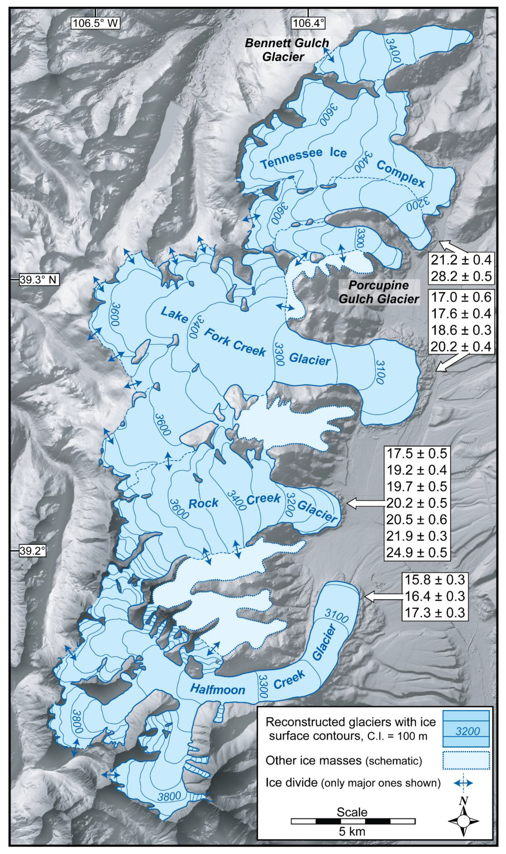
3.2. Glacier Reconstruction

LGM glacier extents and ice surface topographies of six paleoglaciers (Figure 2) were reconstructed on the basis of lateral-terminal moraine complexes and the upper limits of glacial erosion identified by field mapping supplemented by analyses of topographic maps, digital elevation models, and Google Earth® imagery. Where adjacent glaciers shared a common boundary or ice divide, it was assumed to coincide with the existing topographic divide. Of particular note was the difficulty in defining with certainty the ice divides among the paleoglaciers that formed what is referred to here as the Tennessee glacier complex (Figure 2) that is subsequently treated as one system.

Contouring of ice surfaces was guided by considerations of mapped ice limits, flow patterns delineated by large-scale erosional forms, and general convergent and divergent flow in the accumulation and ablations area, respectively. Contours were adjusted iteratively so that reconstructed ice surface slopes were sub-parallel to those of the valley slopes and to ensure driving stresses τ were between 50 and 150 kPa commonly measured on modern glaciers [41]. Stresses were calculated using:

$$\tau = S_{ƒ}\rho gh sin\alpha$$

(1)

where ρ is the density of ice, g is gravitational acceleration, h is ice thickness, α is the slope of the ice surface, and S_ƒ is a shape factor to account for drag of the valley sides [42]. The surface slope was averaged over distances equal to ten-times the local ice thickness to account for longitudinal stress gradients [41,43].

3.3. Temperature-Index Modeling and Simulation of Glacier Mass Balance

Simulation of LGM climate in the northern Sawatch Range uses a temperature-index model (TM) to find the temperature and precipitation changes required to maintain steady-state mass-balances of the reconstructed glaciers. Details of the TM and the justification for its use were given in Brugger et al. [7]. Here, we briefly review the approach and highlight some modifications necessary for the present application.

The variation of the annual specific mass-balance (i.e., at a point) b_n with elevation z is simulated by:

$$b_n\left(z\right)={{\displaystyle \int }}_{t_1}^{t_2}\left(P_s\left(t,z\right)+ M\left(t,z\right)\right)dt$$

(2)

where P_s(t,z) is the rate of snow accumulation, M(t,z) is the rate of snow or ice melt (ablation) over the glacier’s surface during the interval t₁ to t₂ (the hydrologic year). In practice, Equation (2) is numerically integrated over a monthly time-scale to yield monthly melt that is then combined with available monthly precipitation data and then integrated over the hydrologic year.

Melt is determined using a melt (or degree-day) factor m_ƒ that empirically relates ablation to mean daily air temperature T_d(t,z):

$$M\left(z,t\right)=\{\begin{array}{c}{m}_{ƒ}{T}_d\left(t,z\right) T_d\left(t,z\right)>T_m \\ 0 T_d\left(t,z\right)\le T_m\end{array}$$

(3)

where T_m is a threshold temperature above which melting occurs. The advantage of this empirical approach to model snow and ice melt is that it requires fewer meteorological data and other parameterizations than other physically-based approaches (e.g,. energy balance models). More importantly, TMs have proven successful in simulating longer-term ablation over larger spatial scales [44,45,46].

Our simulations were run using a melt threshold temperature T_m of +1 °C, but also 0 °C as these values are typical of other studies [46,47,48,49]. Values of the melt factor m_ƒ for snow and ice are taken as 0.45 and 0.80 cm water equivalent (w.e.) d⁻¹ °C⁻¹ that are reasonable means of values measured on relatively debris-free ice and snow surfaces on modern glaciers [33,50,51]. Although the values of m_ƒ vary spatially and temporally [47,49], they are treated as constants in the present application with m_ƒ initially being set for that of snow but changes to that for ice once snowmelt exceeds accumulation. Because the skill of temperature-index models is sensitive to the choice of m_ƒ [52] we subsequently show that our results are not overly sensitive to their precise value(s).

Daily air temperature is calculated by:

$$T_d\left(z,t\right)= \left[H\left(z\right){\left[\frac{1-\cos \left(\left(\frac{2\pi d}{365}\right)-\varphi \right)}{2}\right]}^k-T_{jan}\left(z\right)\right]-\Delta T$$

(4)

where H(z) is the magnitude of the yearly temperature variation, d is the day of the year, φ is the phase lag (= 0.359 rads), and T_jan(z) is the mean January temperature at elevation z, and ∆T is a prescribed perturbation of mean annual temperature (i.e., LGM temperature depression). Daily air temperatures are then used to determine monthly melt according to Equation (3). The constant k in Equation (4) is a tuning parameter that controls the sharpness of the temperature curve and allowed a better fit to observed temperatures.

Several additional points regarding the implementation of Equation (4) bear mentioning:

(1)

Previously [7,33], H or its equivalent was treated as a constant; however, as alluded to above, PRISM data in the study area reveal a slight systematic decrease with increasing elevation.

(2)

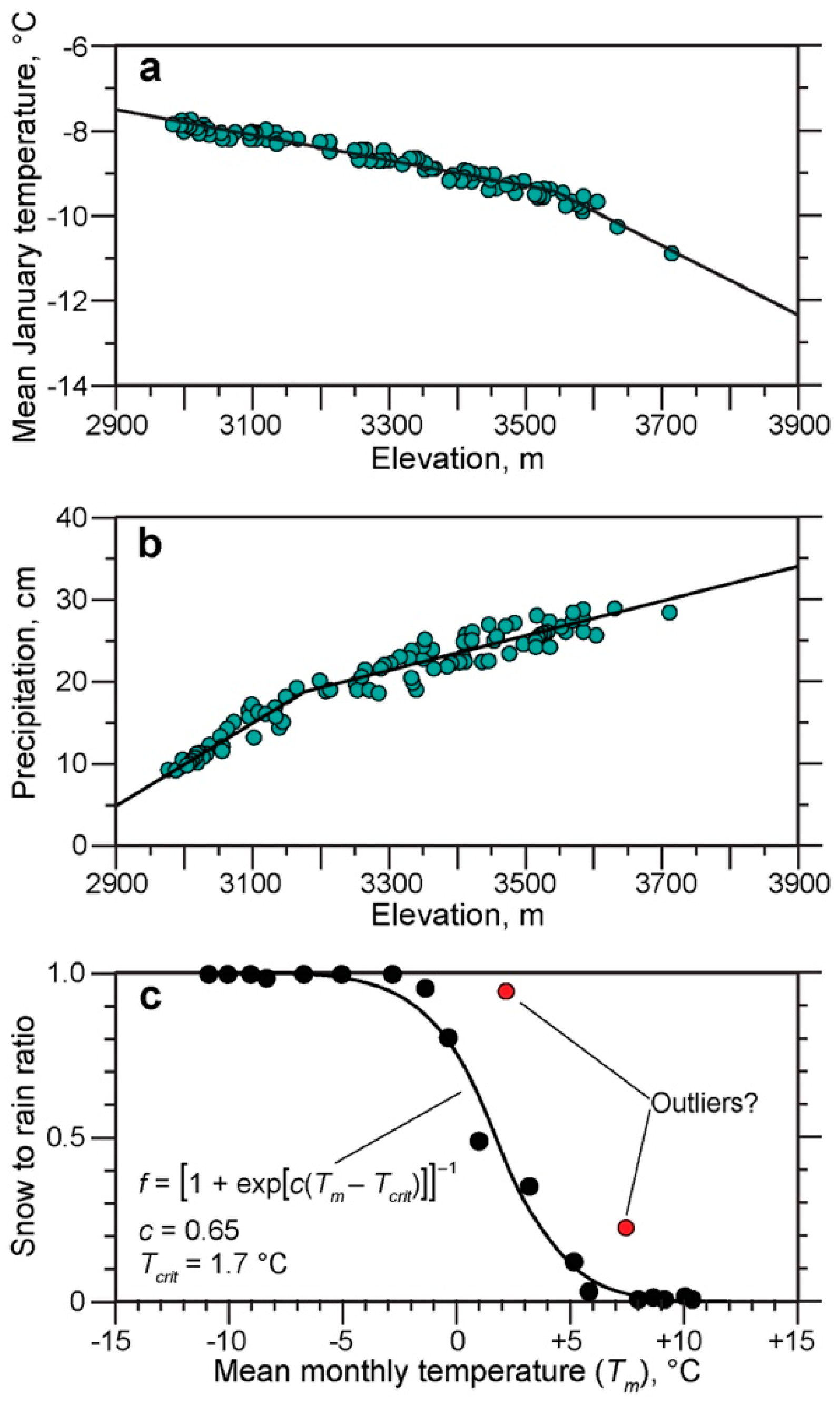
Lacking a sufficient number of meteorological stations—especially at higher elevations—T_jan(z) is determined using the modern lapse rate for January obtained from PRISM climate data (

Table 1. Lapse rates and seasonal precipitation gradients for individual valleys obtained from piecewise linear fits of PRISM climatology. All values are significant at the 95% confidence interval or greater.

Valley	dTjan/dz (°C m−1)	dPWinter/dz (cm m−1)	dPSpring/dz (cm m−1)	dPSummer/dz (cm m−1)	dPFall/dz (cm m−1)
Halfmoon	+0.0005 (<3156 m)	0.0312 (<3449 m)	0.0400 (<3418 m)	0.0108 (<3292m)	0.0296 (<3417 m)
	−0.0048 (>3156 m)	0.0128 (>3449 m)	0.0124 (>3418 m)	0.0027 (>3292 m)	0.0098 (>3417 m)
Rock	−0.0026 (<3469 m)	0.0244 (<3999 m)	0.0297 (<3760 m)	0.0071 (<3182m)	0.0246 (<3770 m)
	−0.0058 (>3469 m)	0.0004 (>3999 m)	0.0138 (>3760 m)	0.0053 (>3182 m)	0.0100 (>3770 m)
Lake Fork	−0.0030 (<3539 m)	0.0363 (<3171 m)	0.0514 (<3168 m)	0.0168 (<3060m)	0.0425 (<3167 m)
	−0.0080 (>3539 m)	0.0228 (>3171 m)	0.0210 (>3168 m)	0.0034 (>3060 m)	0.0174 (>3167 m)
Porcupine	−0.0042 (<3307 m)	0.0197 (<3244 m)	0.0256 (<3257 m)	0.0116 (<3229m)	0.0176 (<3267 m)
	−0.0019 (>3307 m)	0.0268 (>3244 m)	0.0321 (>3257 m)	0.0215 (>3229 m)	0.0236 (>3267 m)
Tennessee	−0.0035 (<3482 m)	0.0246 (<3567 m)	0.0301 (<3565 m)	0.0146 (<3160m)	0.0199 (<3560 m)
	−0.0058 (>3482 m)	0.0073 (>3567 m)	0.0090 (>3565 m)	0.0028 (>3160 m)	0.0057 (>3560 m)
Bennett	−0.0016 (<3423 m)	0.0152	0.0198	0.0039	0.0114
	−0.0075 (>3423 m)	-	-	-	-

) sampled over the extent of glacier surfaces in conjunction with a value of T_jan(z) at some reference elevation. PRISM data suggest two different lapse rates should be used in each valley according to the elevation interval under consideration, therefore data were fit using piecewise linear splines (Figure 3). The fitting routine [53] yields a continuous function that optimizes the elevation of the breakpoints (or knots) in the linear fits. Use of the spline fits resulted in slightly better agreement between the modeled and PRISM temperatures than did simple linear regressions.

(3)

Equation (4) also implies a uniform perturbation of temperature ∆T over the year, hence no temperature seasonality is examined in the present study.

(4)

Values of k in the valleys studied varied between 1.18 and 1.20 and were chosen to minimize the difference between simulated mean monthly temperatures and those obtained from the PRISM data and any relevant meteorological station(s) during the ablation season (May through September). Priority is given to the ablation season because of the temperature dependence of melting in the TM.

Snow accumulation P_s(t,z) is determined by:

P_s(t,z) = ƒP_mod(t,z) + F

(5)

where P_mod(t,z) is the modern precipitation, ƒ is a function that determines what fraction of monthly precipitation falls as snow based on the air temperature (Figure 3c), and F is a prescribed change in precipitation (i.e., assumed changes in precipitation during glaciation). Values for P_mod(t,z) are calculated from the monthly fraction of the respective seasonal (winter, spring, summer, fall) totals and corresponding vertical precipitation gradients (Table 1). Here, it was particularly useful to fit the seasonal PRISM data using piecewise linear splines (Figure 3), substantially improving the agreement between modeled precipitation and PRISM data (the exceptions were the PRISM precipitation data for Bennett Gulch that were fitted using simple linear regression). This reflects the fact that while precipitation is dependent on elevation it is also influenced by the location, orography aspect, and other factors [54]. The “bounding” elevation (i.e., the breakpoint) was in some cases seasonally consistent (especially for winter, spring and fall) and in others not. While seasonal precipitation gradients are distinct, intraseasonal variations are small. Monthly fractions of seasonal precipitation only vary by ~5% during the accumulation season and show no significant trend with elevation.

4. Results

4.1. ¹⁰Be Cosmogenic Exposure Ages

Individual zero-erosion ages of the sixteen boulders sampled on LGM terminal moraines in the study area are shown in Figure 2. The seven boulders on the terminal moraine in Rock Creek valley yielded a mean ¹⁰Be age of 20.6 ± 2.3 ka. Boulders on the Lake Fork and Halfmoon Creek moraines have mean ages of 18.4 ± 1.4 (n = 4) and 16.5 ± 0.8 ka (n = 3) respectively. The older of the two boulders sampled in Longs Gulch, having an age of 28.2 ka, is considered an outlier from the other fifteen ages because of the probable ¹⁰Be inheritance. Excluding the latter, boulder ages on terminal moraines span an interval of 24.9 to 15.8 ka. However, in the Halfmoon Creek valley the boulders sampled are upvalley from the outermost crest of the terminal moraine. This is also the case for the three younger ages on the Lake Fork terminal moraine, while the boulder having the oldest age (20.2 ka) is on the distal toe of the moraine. This suggests that these younger ages might not date the local LGM but rather the persistence of ice at, or close to, the glaciers’ maximum extent.

4.2. Glacier Reconstructions

Pertinent characteristics of the six glacier reconstructions (Figure 2) are presented in

Table 2. Surface areas, lengths, thicknesses, mean slope of ice surfaces, mean driving stresses, and equilibrium-line altitudes (ELAs) of reconstructed glaciers.

Glacier	Area, km2	Length, km*	Average Thickness, m†	Maximum Thickness, m†	Average Slope, Degrees	Average Driving Stress, kPa	AAR-Derived ELA†
Halfmoon Creek	44.3	16.7	120	240	4.8	87	3475
Rock Creek	29.0	10.9	80	150	7.6	100	3385
Lake Fork Creek	63.6	15.0	140	260	4.2	100	3365
Porcupine Gulch	5.8	7.0	75	125	5.7	77	3310
Tennessee complex	38.2	9.7	80	150	6.0	84	3360
Bennett Gulch	8.3	6.9	75	115	5.6	79	3345

* Longest flow line; ^† Nearest 5 m.

. As expected, average and maximum ice thickness generally scale with glacier size. Driving stresses largely varied according to the product of slope and ice thickness (Equation (1)), the shape factor being relatively constant (~0.8–0.9). Larger stresses are typically associated with thicker ice in the mid-reach of the glaciers and/or steeper surface slopes found at their heads. Conversely, lower stresses tend to be associated with thinner ice at glacier termini. Of the 154 calculated values only eighteen fell outside the range of 50–150 kPa, the minimum and maximum stresses being 45 and 169 kPa respectively. Reconstructed ice surface hypsometry also allowed determination of the equilibrium-line altitudes (ELAs) of paleoglaciers using the accumulation-area ratio (AAR) method. Here we used an AAR value of 0.65 [7,33]. ELAs were consistent averaging 3375 ± 55 m.

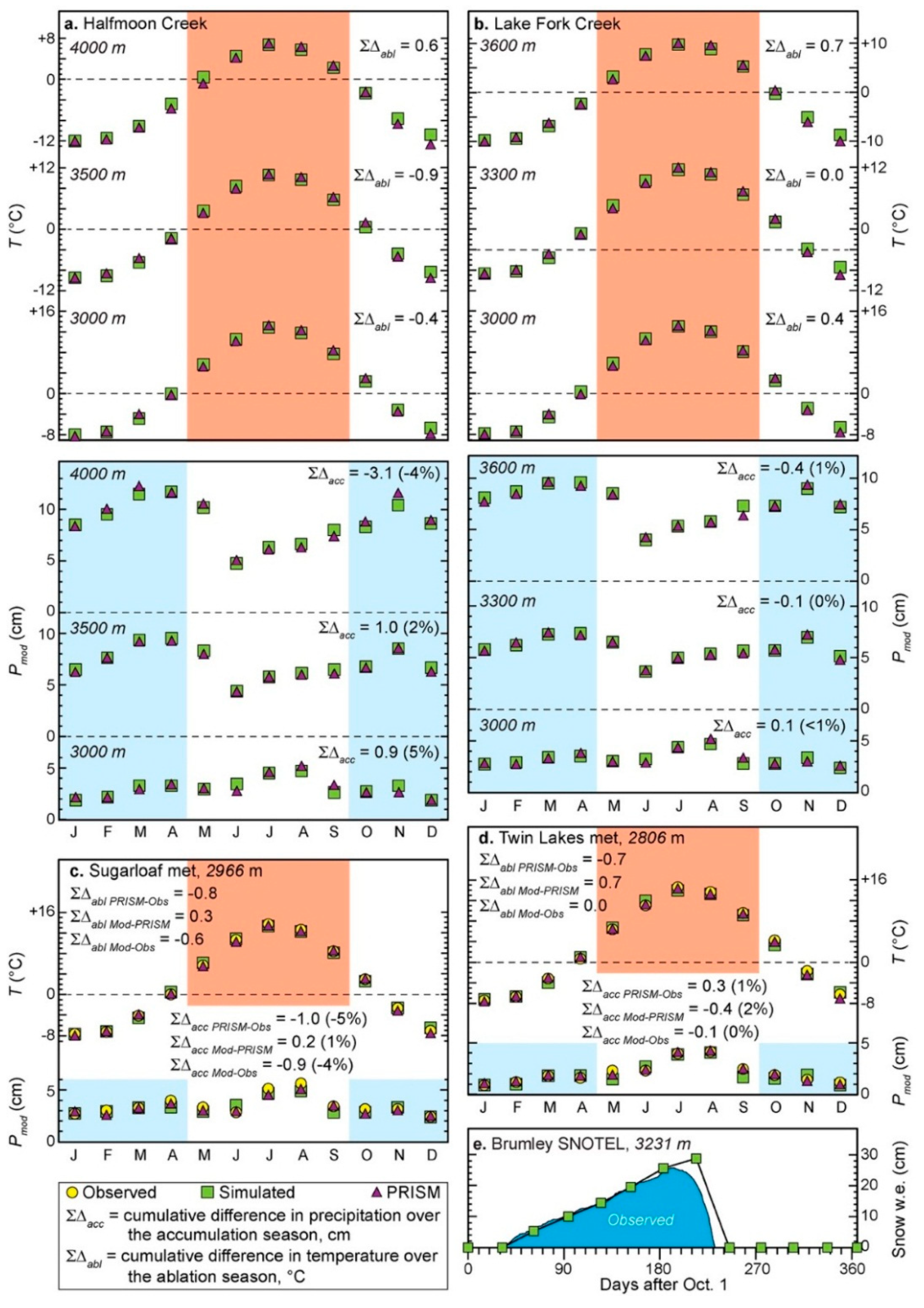
4.3. Temperature-Index Modeling: Model Skill

Model skill was first evaluated by simulation of modern climate. The objective here is to determine how accurately the model, with the parameterization described above, captures the area-averaged temperature and precipitation given by the PRISM gridded climatology (1981–2010 normals). For monthly temperature and precipitation values, averages were obtained from several spot locations chosen from the PRISM data corresponding to a particular elevation (

Table 3. Comparison of modeled modern temperature and precipitation with PRISM values at select elevations in the study area. Percentages are rounded to the nearest whole number or noted when less than one percent. Elevation ranges shown account for ≥90% of glacier areas. Values in bold are most significant in terms of modeling paleoglacier mass balances.

Climate Parameters and Differences	Values
Rock Creek
Elevation, m (number of PRISM locations averaged)	3000 (n = 5)	3250 (n = 6)	3500 (n = 6)	3750 (n = 6)	4000 (n = 4)
Modeled mean annual temperature, °C	1.8	0.9	0.0	−1.7	−3.3
PRISM mean annual temperature, °C	1.8 ± 0.0	1.0 ± 0.0	−0.1 ± 0.1	−1.9 ± 0.1	−3.7 ± 0.0
Difference, °C	0.0	−0.1	0.1	0.2	0.4
Mean ± standard deviation of monthly differences, °C	0.0 ± 0.5	−0.5 ± 0.6	0.1 ± 0.7	0.2 ± 0.7	0.3 ± 0.7
Cumulative difference temperatures during ablation season, °C	−0.2	−0.2	<−0.1	<0.1	0.5
Modeled mean annual precipitation, cm	41.1	62.4	83.4	103.9	118.3
PRISM mean annual precipitation, cm	40.4 ± 1.1	62.5 ± 3.8	83.2 ± 5.1	105.8 ± 3.2	117.7 ± 3.3
Difference, cm (%)	0.6 (1%)	−0.1 (<1%)	0.2 (<1%)	−1.9 (2%)	0.6 (1%)
Mean ± standard deviation of monthly differences, cm	0.1 ± 0.4	0.0 ± 0.2	0.0 ± 0.2	−0.2 ± 0.5	0.1 ± 0.7
Cumulative difference in precipitation during accumulation season, cm (%)	1.1 (5%)	0.3 (<1%)	−0.2 (<1%)	−2.0 (3%)	−2.0 (<1%)
Halfmoon Creek
Elevation, m (number of PRISM locations averaged)	3000 (n = 4)	3250 (n = 7)	3500 (n = 11)	3750 (n = 16)	4000 (n = 9)
Modeled mean annual temperature, °C	1.7	1.1	−0.3	−1.8	−3.2
PRISM mean annual temperature, °C	1.8 ± 0.0	0.9 ± 0.1	−0.2 ±0.1	−1.8 ± 0.1	−3.6 ± 0.1
Difference, °C	−0.1	0.2	−0.1	0.0	0.4
Mean ± standard deviation of monthly differences, °C	0.0 ± 0.6	0.2 ± 0.6	−0.1 ± 0.7	0.0 ± 0.7	0.4 ± 0.8
Cumulative difference temperatures during ablation season, °C	−0.4	1.2	−0.9	−0.9	0.6
Modeled mean annual precipitation, cm	36.6	64.5	85.9	95.3	104.7
PRISM mean annual precipitation, cm	36.5 ± 1.9	68.7 ± 7.1	84.1 ± 7.5	96.4 ± 5.6	107.5 ± 10
Difference, cm (%)	0.1 (<1%)	−4.2 (6%)	1.7 (2%)	−1.1 (1%)	−2.8 (3%)
Mean ± standard deviation of monthly differences, cm	0.0 ± 0.4	−0.4 ± 0.3	0.1 ± 0.2	−0.1 ± 0.3	−0.2 ± 0.5
Cumulative difference in precipitation during accumulation season, cm (%)	0.9 (5%)	−3.0 (7%)	1.0 (2%)	−1.7 (3%)	−3.1 (4%)
Lake Fork Creek
Elevation, m (number of PRISM locations averaged)	3000 (n = 5)	3150 (n = 8)	3300 (n = 9)	3450 (n = 15)	3600 (n = 10)
Modeled mean annual temperature, °C	2.0	1.4	0.8	0.2	−0.7
PRISM mean and stand deviation of annual temperature, °C	1.9 ± 0.0	1.3 ± 0.0	0.7 ± 0.1	0.1 ± 0.1	−0.7 ± 0.1
Difference, °C	0.1	0.1	0.1	0.1	0.0
Mean ± standard deviation of monthly differences, °C	0.1 ± 0.5	0.1 ± 0.6	0.0 ± 0.7	0.1 ± 0.7	0.0 ± 0.7
Cumulative difference temperatures during ablation season, °C	0.4	0.4	0.0	−0.2	−0.7
Modeled mean annual precipitation, cm	39.3	59.0	71.0	80.7	90.4
PRISM mean and standard deviation of annual precipitation, cm	39.8 ± 1.4	57.8 ± 4.0	70.9 ± 5.4	81.6 ± 5.9	89.2 ± 2.9
Difference, cm (%)	−0.5 (1%)	1.2 (2%)	0.1 (<1%)	−0.9 (1%)	1.1 (1%)
Mean ± standard deviation of monthly differences, cm	0.0 ± 0.3	0.1 ± 0.1	0.0 ± 0.2	0.0 ± 0.3	0.1 ± 0.4
Cumulative difference in precipitation during accumulation season, cm (%)	0.1 (<1%)	1.0 (3%)	−0.1 (<1%)	−0.7 (1%)	0.4 (1%)
Tennessee Creek/Longs Gulch
Elevation, m (number of PRISM locations averaged)	3100 (n = 5)	3300 (n = 8)	3500 (n = 8)	3700 (n = 8)
Modeled mean annual temperature, °C	1.5	0.7	−0.2	−1.4
PRISM mean and stand deviation of annual temperature, °C	1.4 ± 0.0	0.7 ± 0.1	0.0 ±0.1	−1.5 ± 0.1
Difference, °C	0.1	0.0	−0.2	0.1
Mean ± standard deviation of monthly differences, °C	0.1 ± 0.6	0.0 ± 0.7	−0.1 ± 0.7	0.0 ± 0.6
Cumulative difference temperatures during ablation season, °C	−0.6	−0.4	−0.6	0.4
Modeled mean annual precipitation, cm	53.1	69.4	84.9	93.2
PRISM mean and standard deviation of annual precipitation, cm	53.0 ± 0.7	69.6 ± 1.3	84.8 ± 5.9	94.1 ± 3.0
Difference, cm (%)	−0.5 (1%)	−0.6 (1%)	−0.7 (1%)	−0.8 (1%)
Mean ± standard deviation of monthly differences, cm	0.0 ± 0.3	0.0 ±0.1	0.0 ± 0.2	-0.1 ± 0.4
Cumulative difference in precipitation during accumulation season, cm (%)	0.6 (2%)	−0.3 (1%)	−0.2 (<1%)	−1.2 (2%)
Bennett Gulch
Elevation, m (number of PRISM locations averaged)	3200 (n = 4)	3350 (n = 5)	3500 (n = 5)	3650 (n = 1)
Modeled mean annual temperature, °C	1.1	0.8	0.0	−1.3
PRISM mean and stand deviation of annual temperature, °C	1.0 ± 0.1	0.8 ± 0.1	0.0 ± 0.0	−1.2
Difference, °C	0.1	0.0	0.0	−0.1
Mean ± standard deviation of monthly differences, °C	0.1 ± 0.7	−0.1 ± 0.7	−0.1 ± 0.7	0.0 ± 0.7
Cumulative difference temperatures during ablation season, °C	0.3	0.0	0.0	−0.3
Modeled mean annual precipitation, cm	62.7	70.2	77.8	85.3
PRISM mean and standard deviation of annual precipitation, cm	61.9 ± 1.2	71.5 ± 2.0	77.2 ± 1.8	85.0
Difference, cm (%)	0.6 (1%)	-1.3 (2%)	0.6 (1%)	0.3 (<1%)
Mean ± standard deviation of monthly differences, cm	0.1 ± 0.1	-0.1 ± 0.1	0.1 ± 0.2	0.0 ± 0.3
Cumulative difference in precipitation during accumulation season, cm (%)	0.8 (2%)	−1.1 (2%)	0.2 (<1%)	−0.3 (1%)
Porcupine Gulch
Elevation, m (number of PRISM locations averaged)	3100 (n = 3)	3250 (n = 3)	3400 (n = 4)	3550 (n = 3)
Modeled mean annual temperature, °C	1.5	0.8	0.3	0
PRISM mean annual temperature, °C	1.4 ±0.0	0.8 ± 0.0	0.4 ± 0.1	−0.2 ± 0.0
Difference, °C	0.1	0	−0.1	0.2
Mean ± standard deviation of monthly differences, °C	0.1 ± 0.6	0.0 ± 0.7	0.0 ± 0.7	0.1 ± 0.7
Cumulative difference temperatures during ablation season, °C	0.4	−0.4	−0.7	0.7
Modeled mean annual precipitation, cm	52	62.4	75.7	88.4
PRISM mean annual precipitation, cm	52.5 ± 0.4	63.8 ± 2.5	75.4 ± 3.3	87.2 ± 3.2
Difference, cm (%)	−0.5 (1%)	−0.4 (1%)	0.3 (< 1%)	1.1 (1%)
Mean ± standard deviation of monthly differences, cm	0.0 ± 0.2	0.0 ± 0.1	0.0 ± 0.2	0.1 ± 0.4
Cumulative difference in precipitation during accumulation season, cm (%)	0.0 (<1 %)	−0.5 (1%)	−0.1 (<0%)	0.3 (1%)

) (it should be emphasized that the model uses the PRISM data only to determine lapse rates and vertical precipitation gradients; that is temperature or precipitation is not prescribed but rather determined using Equation (4)). The number of locations chosen (given in Table 3) varied according to the extent of glacier area at those elevations and were spaced to ensure they represented variations over that area.

The model simulates modern climate quite well in terms of mean annual and monthly temperatures and precipitation (Table 3 and Figure 4a,b). Modeled MATs typically differ from PRISM values by less than 0.2 °C. Mean monthly temperature differences are also small. This is not surprising given the strong dependence of temperature on elevation, evidenced by the small standard deviations in the mean annual PRISM temperatures (Table 3). Differences in MAPs and monthly precipitation amounts are more variable (cf. standard deviations associated with PRISM MAPs) because of the influence of other factors in conjunction with elevation. Nonetheless, the differences between modeled and PRISM MAPs are small, only in one instance exceeding 5%. Mean monthly differences are again small. Arguably however, for the application of the TM to simulate glacier mass balances, the most relevant comparisons are between the cumulative temperature differences during the “ablation season” (May–September) and the cumulative difference in precipitation during the “accumulation season” (October–April). For all valleys in the study area, these differences average ~0.5 °C and ~2% respectively. It bears mentioning that average differences in ablation season temperature would be significantly less (~0.3 °C) if not for the higher values in the Halfmoon Creek valley (Table 3). Similarly, comparisons were made between modeled temperature and precipitation and the 1981–2010 climate normals for the Sugarloaf and Twin Lakes meteorological stations (Figure 4c,d) using parameterizations specific to those locations. Agreement between observed and modeled monthly and annual means is quite good.

Model performance can also be evaluated by comparing the simulated snowpack evolution with that observed at SNOTEL stations. Modeling of snow accumulation and melt is more closely related to the goal of simulating glacier mass balance. Unfortunately, the Brumley SNOTEL is the only nearby site on the eastern slope of the northern Sawatch Range, and it lies immediately outside the study area (Figure 1). Nevertheless, again using valley specific parameterization the TM simulates observed modern snowpack evolution quite well (Figure 4e) with due consideration of differences in temporal resolution (monthly versus daily respectively) and other factors affecting the snow accumulation and melt in SNOTEL settings (see [7]). Varying the melt factor m_ƒ by ± 0.002 m w.e. d⁻¹ °C⁻¹ has the net effect of changing the maximum snowpack by no more than ± 5%. This is because melting (i.e., positive degree-days) only occurs after late April. Likewise, the melt threshold has virtually no impact on snowmelt because its effect is limited to the very short transition from the accumulation to ablation seasons and vice versa.

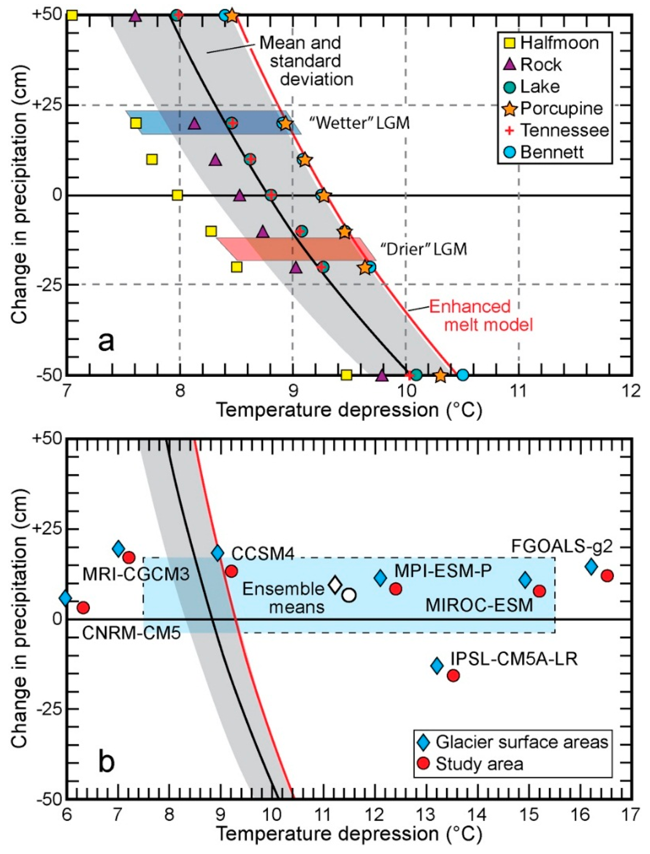
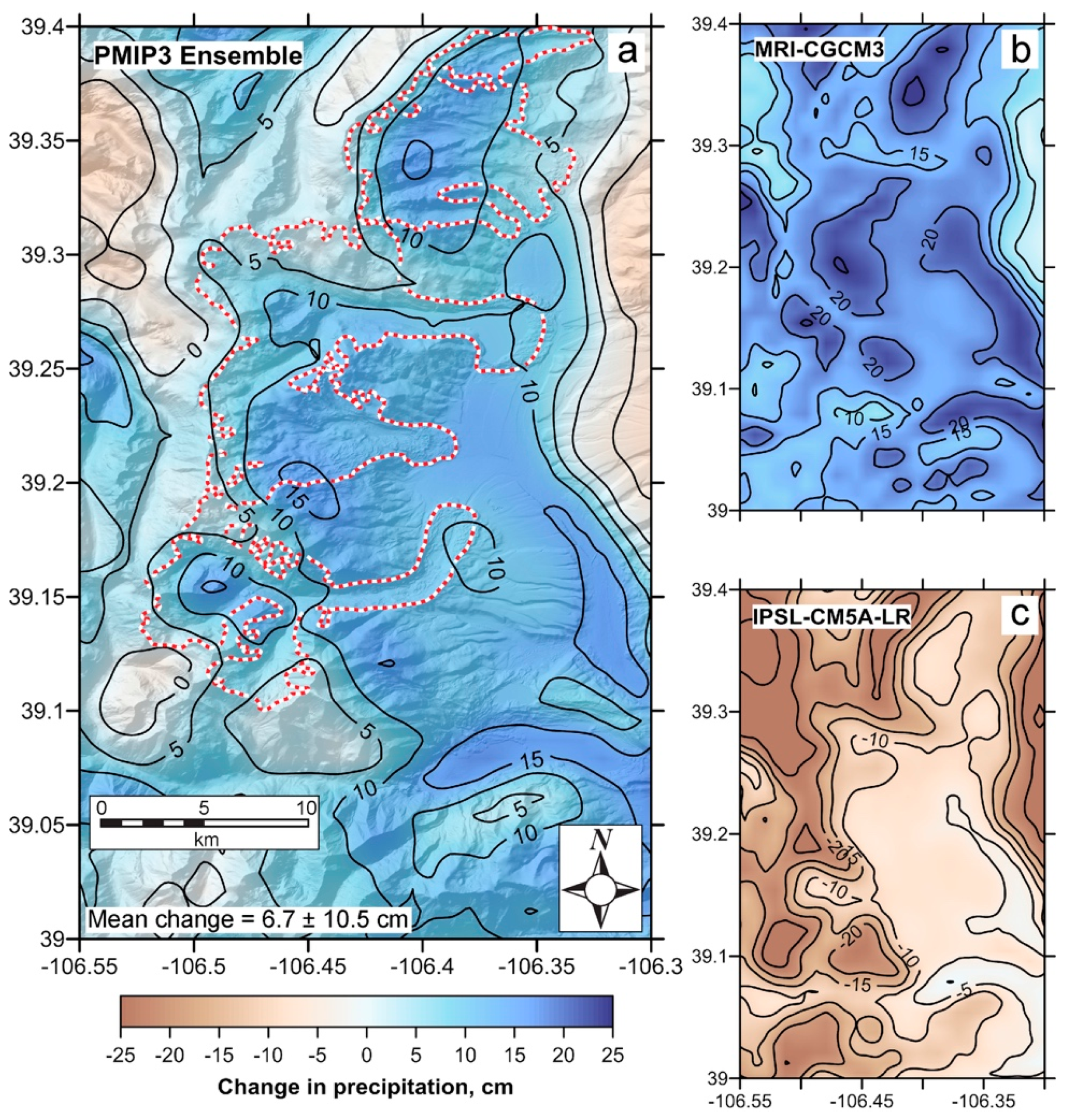
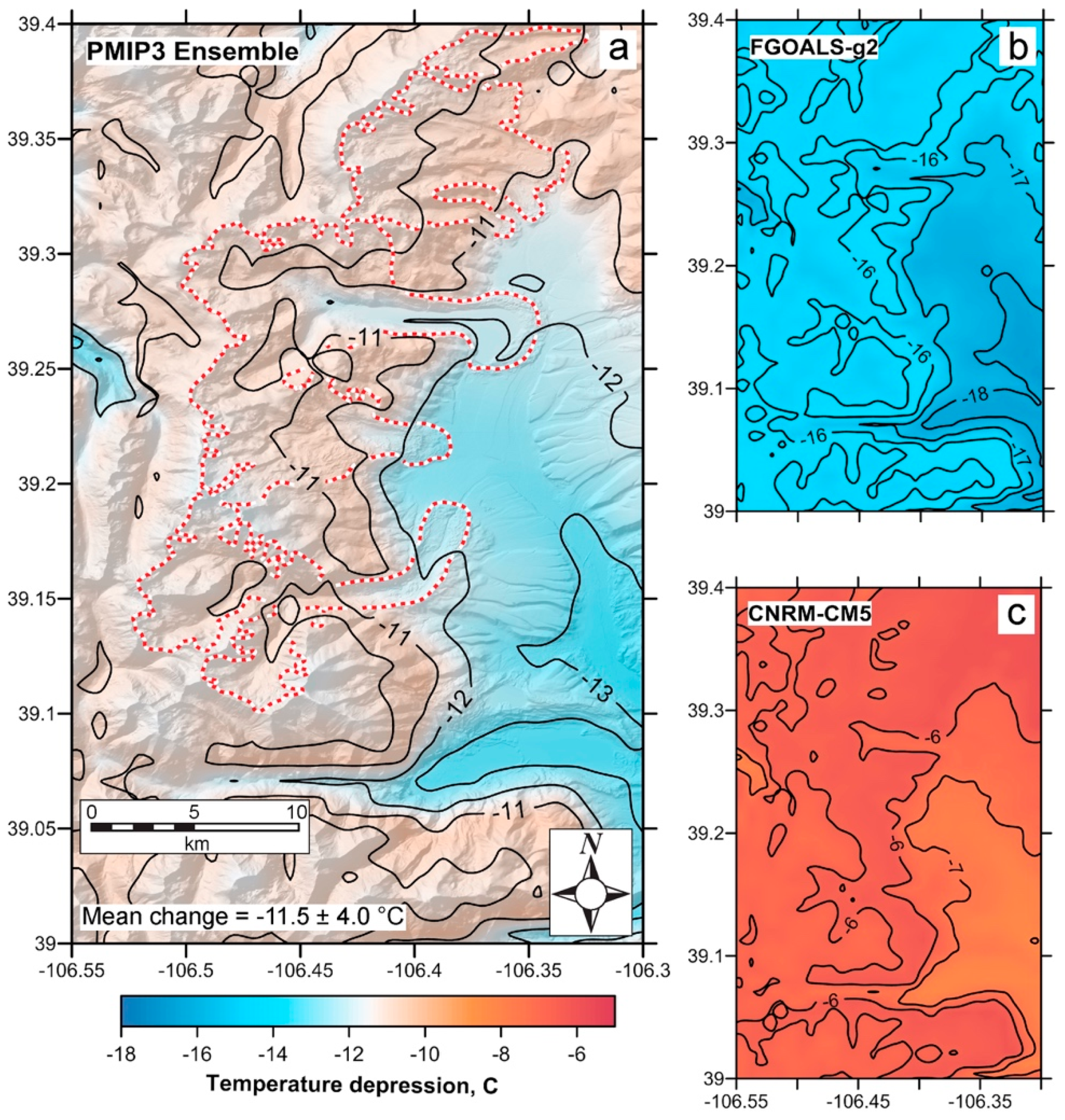
4.4. Temperature-Index Modeling: Inferring Late Pleistocene Glacial Climate

Climate during the last glaciation is determined by finding the temperatures and/or precipitation that satisfy:

$$B_n=\underset{A}{\overset{ }{{\displaystyle \int }}}{b}_{n}dA \approx {\displaystyle \sum }_{i=1}^j{b}_{n_i}{A}_i=0$$

(6)

where B_n is the steady-state mass-balance, A is glacier area composed of j number of discrete elevation intervals, and $b_{n_i}$ is the mean annual specific net-balance over A_i. Equation (6) explicitly considers glacier hypsometry.

In solving Equation (6), the problem of equifinality arises in that infinite combinations of temperature depression and precipitation changes satisfy the condition B_n = 0. Therefore, assumptions must be made regarding LGM precipitation in the study area. Lacking robust precipitation proxies, it remains unclear whether the study area was wetter or drier than present during the glacial maximum. Moreover, regional climate modeling [26,28,55] suggests the possibility of modest changes in either direction. Therefore, we initially determine mass balances required to maintain steady-state of the six paleoglaciers at their LGM extents by assuming LGM precipitation and its seasonal distribution were comparable to today. We then examine the cases for reasonable increases or decreases in precipitation.

Assuming no change in precipitation, temperature depressions ranged from 8.0 to 9.3 °C, the mean being 8.8 ± 0.5 °C (

Table 4. Derived temperature depressions and ELAs based on steady-state mass balance of paleoglaciers. Temperatures are reported to the nearest tenth of a degree.

Model Parameter	Temperature Depression, °C					Steady-State ELA, m*
Precipitation change (F), cm		0		10	–10
Melt factors (mf), snow/ice, m w.e. °C−1 d−1	0.0045/0.008	0.006/0.010	0.0025/0.006	0.0045/0.008
Glacier
Halfmoon Creek (southernmost)	8.0	8.4	7.2	7.8	8.2	3500
Rock Creek	8.5	8.9	7.8	8.3	8.7	3470
Lake Creek	8.8	9.2	8.1	8.6	9.0	3410
Porcupine Gulch	9.3	9.6	8.6	9.1	9.4	3345
Tennessee complex	8.8	9.2	8.1	8.6	9.0	3435
Bennett Gulch (northernmost)	9.2	9.7	8.6	9.1	9.5	3435
Means	8.8 ± 0.5	9.2 ± 0.5	8.1 ± 0.5	8.6 ± 0.5	9.0 ± 0.5	3435 ± 55

* For F = 0, m_ƒ = 0.0045/0.008 m °C⁻¹ d⁻¹.

; Figure 5a). Although the inferred temperature depressions hint at a south-to north increase in LGM cooling, consistent with large-scale climate modeling, the associated uncertainties (discussed subsequently) preclude a firm conclusion regarding the coherency of any spatial trend. The ELAs associated with steady-state mass balances average ~60 m higher than those based on the AAR ratio.

Changes in LGM precipitation of ± 10 cm with respect to modern MAPs (equivalent to ~10–25% depending on elevation and location) require greater/smaller temperature depression to compensate for reductions/increases in snow accumulation. Changes of this magnitude are considered most reasonable given what is suggested by regional climate modeling [26,28,55]. These changes, however, only alter the inferred temperature depressions by ~ ±0.2 °C (Table 4). The effect of more “extreme” changes in LGM precipitation on required temperature depressions is shown in Figure 5a. For example, with changes of ±20 cm, steady-state mass balances of individual glaciers require temperature depressions ranging from ~7.6 to 9.7 °C respectively (mean values are 8.5 and 9.2 °C).

Associated uncertainties are estimated via sensitivity analysis to be + 0.5/– 0.8 °C (

Table 5. Sensitivity of TM simulations to variations of parameter values and resulting uncertainties, grouped by whether the variation increases (positive values) or decreases (negative values) the temperature depression required to maintain steady-state mass balances of paleoglaciers.

	Parameter
	Potential Change in LGM Precipitation, (F) cm	Melt Threshold Temperature, °C	Melt Factors (mf), cm w.e. d−1 °C−1	Effect of Glacier Hypsometry Error, °C	Total*
Initial value	0.0	+1.0	ice 0.0080 snow 0.0045	-
Variation	±10	0.0	±0.002	±0.2
Effects, °C	+0.2	0.0	+0.7	+0.2	+0.8
	−0.2	0.0	−0.4	−0.2	−0.5

* Added in quadrature.

). The greatest source of uncertainty arises from potential variations in the value of the melt factors for snow and ice. Other contributions are equally distributed among uncertainties in precipitation and reconstructed glacier hypsometry. Allowing precipitation to vary not only addresses changes that might have potentially occurred during the LGM but can also account for changes in its seasonal distribution, vertical gradient(s), and the fraction that falls as snow—all affecting accumulation hence glacier mass balance [7,33]. Uncertainty attributed to those in glacier hypsometry is based on a Monte Carlo simulation wherein a Gaussian distributed error for the area of each elevation interval was allowed to vary by ±20%.

5. Discussion

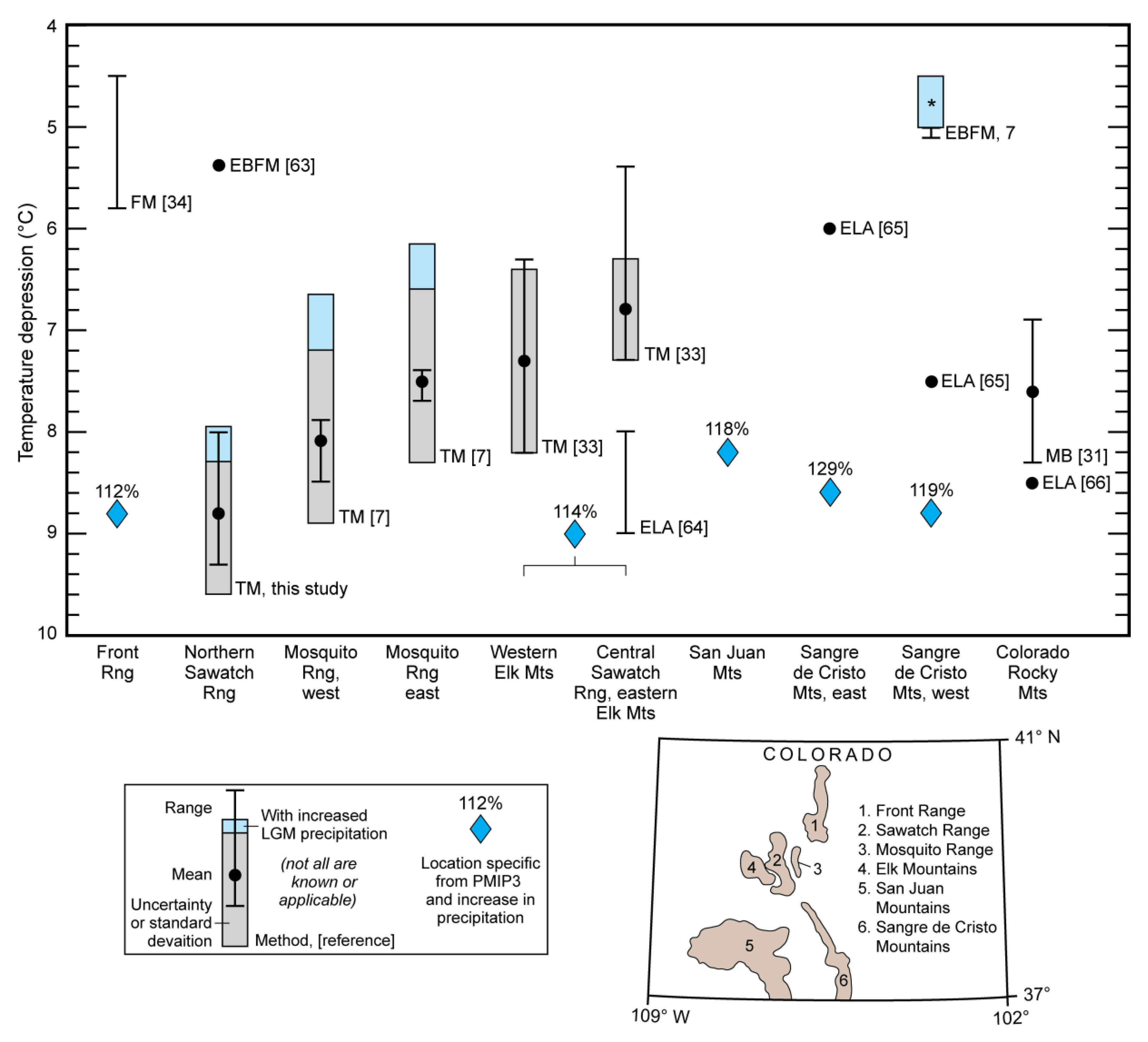
5.1. Chronology of the Local LGM

Considering uncertainties (Table S1) and the presumed outlier, overlapping boulder ages appear to define two dominant populations, the means of which are 20.2 ± 1.1 ka (n = 8) and 16.9 ± 0.7 ka (n = 6). Inclusion of an older age (24.9 ka) in the former yields a mean of 20.7 ± 1.9 ka. Thus we consider the local LGM in the northern Sawatch Range to have occurred ~20–21 ka. This is very consistent with the age of LGM advances in the immediately adjacent Mosquito Range [7] and throughout the Colorado Rocky Mountains [10].

The significance of the younger population is uncertain at this time. As noted previously, however, these ages are from boulders that are typically in more proximal positions on their respective terminal moraines, and a tentative conclusion is that they represent stillstands or slight readvances at ~16.9 ka. Similar ages on recessional moraines in the Mosquito Range [7] and in other ranges in Colorado [10] document near maximum extents of glaciers at this time. Brugger et al. [7] suggested this was possibly in response to the Heinrich Stadial 1 cooling [7].

5.2. Regional LGM Temperature Depression and Constraints on Precipitation

Simulations of steady-state mass balances of the six paleoglaciers in the northern Sawatch Range suggest that climate during the LGM was characterized by mean annual temperatures ~8.8 ± 0.5 °C cooler than present if there were no significant changes in precipitation. Assuming a slightly wetter or drier LGM (F = ±10 cm), consistent with simulations of regional climate, the means of required temperature depression are 8.7 ± 0.5 and 9.1 ± 0.5 °C respectively (Figure 5a).

Unfortunately, no other proxies for LGM climate exist in the study area for comparison. Therefore, we compare our results to the PMIP3 (Paleoclimate Modeling Intercomparison Project Phase 3) LGM climate simulations. Because of the coarse resolution of the PMIP3 models (i.e., the study area is subgrid), we make use of the CHELSA (Climatologies at High Resolution for the Earth’s Land Surface Areas; [56,57]) downscaled PMIP3 model output that has a resolution of 30 arc sec (~1 km). Regional downscaling suffers from biases inherent in the “parent” global models but can be particularly advantageous in capturing climate in terrain characterized by high relief [58,59]. Downscaling is available for seven models: NCAR-CCSM4, MRI-CGCM3, CNRM-CM5, FGOALS-g2, IPSL-CM5A-LR, MIROC-ESM, and MPI-ESM-P. Departures of LGM MATs and MAPs from the present are determined using the CHELSA modern climatology (defined as 1979–2013). The rationale for using the latter instead of the PRISM climatology is that the same downscaling methods are employed. Differences in the two modern climatologies are such that, on average in the study area, PRISM climatology is characterized by MATs ~0.75 °C cooler and MAPs ~24 cm greater than the CHELSA climatology. We make no formal corrections to account for differences between preindustrial temperatures to which PMIP models are referenced and current temperatures (1986–2005) that are estimated to be 0.55–0.8 °C warmer [60]. Presumably therefore, LGM temperature changes from modern presented here are slight overestimates.

LGM MATs and MAPs derived from individual models vary in magnitude over the study area. Average MATs (n = 1650) range from −6.7 °C (CNRM-CM5) to as low as −16.9 °C (FGOALS-g2) with an ensemble mean of −11.9 °C. Average MAPs range from a low of 27.5 cm (FGOALS-g2) to a high of 59.2 cm (MRI-CGCM3) with an ensemble mean of 49.2 cm. CHELSA modern climatology yields a mean MAT of −0.4 °C and MAP of 42.6 cm.

Most relevant to the present study are the possible changes in MAP and MAT in the study area suggested by the downscaled PMIP3 models. Figure 6 and Figure 7 respectively show changes in LGM MAP and temperature depression based on ensemble mean values, and for the driest/warmest and wettest/coolest scenarios. While not surprising, the magnitude of these changes vary but the spatial patterns are quite similar owing to a degree of elevational dependence. In general, greater increases in MAP and greater temperature depressions are indicative of lower elevations (i.e., valleys). With the exception of IPSL-CA5-LR that suggests a reduction in MAP averaging −15.1 cm, all other models show increases ranging from +3.0 (CNRM-CM5) to +16.6 cm (MRI-CGCM3); the ensemble mean is +6.7 cm (Figure 5b and Figure 6). The potential changes in MAP indicated by the downscaled PMIP3 models address in particular a key unknown in attempting to determine temperature depressions necessary to maintain steady-state mass balances of the paleoglaciers in the northern Sawatch Range. Despite the uncertainties in those models, it would appear that the most likely LGM scenario was one of increased precipitation. Clipping the CHELSA grids to the areas of individual ice masses (shown in Figure 6a) suggests an increase of ~10 cm. However, as noted previously, an increase of this magnitude is inconsequential for the estimates of LGM temperature depression (Table 4 and Figure 5a). The wettest scenario (Figure 6b), corresponding to an increase in MAP of ~20 cm greater than modern, requires a mean temperature depression of ~8.5 °C (Figure 5a) for steady-state mass balances. In contrast, the driest scenario (Figure 6c) that corresponds to a decrease in MAP of ~15 cm over glacier areas, requires a cooling of ~9.2 °C.

The downscaled PMIP3 ensemble mean suggests that average MATs might have been 11.5 °C (or 11.2 °C if grids are clipped to glacier areas) cooler than present (Figure 5b and Figure 7), with estimates from individual models between 6.3 (CNRM-CM5) and 16.5 °C (FGOALS-g2). However, Figure 5a reveals that temperature depressions greater than 10 °C would require substantial decreases in LGM precipitation—exceeding 50 cm—in order to maintain steady-state glacier mass balances. Reductions of this magnitude are problematic, especially at lower elevation where today MAPs are 40–60 cm. This begs the question whether the large temperature depressions suggested by several of the downscaled PMIP3 models (Figure 5b) can be reconciled without seemingly improbable reductions in MAP. To explore one possibility, we ran an “enhanced melt” simulation (Figure 5a) of paleoglacier mass balance, the reasoning being that greater melt would necessitate less reduction in MAP, or more specifically snow accumulation. Toward that end, these simulations used higher melt factors (m_ƒ = 0.65, 1.0 cm w.e. d⁻¹ °C⁻¹ for snow, ice), a lower threshold temperature for melt (T_m = −1 °C), and the hypsometry of the Lake Fork Creek paleoglacier because results for the latter closely match the mean of the group. Even with these constraints, unrealistic reductions in LGM precipitation are implied for temperature depression exceeding ~10.5 °C. We also considered a scenario in which the seasonal distribution of precipitation changed while MAPs over all elevations remained constant. Specifically, if 50% of winter and 25% of spring precipitation fell during the summer (hence lessening snow accumulation), the required temperature depressions are ~1 °C cooler than those shown in Figure 5a. Thus given (1) temperature depressions greater than ~10 °C require extraordinary reductions in precipitation, (2) that six of the seven downscaled PMIP3 models suggest that LGM climate was likely wetter (Figure 5b), and (3) considering uncertainties, our estimates of 8.1–9.2 °C (means in Table 1) appear to be robust measures of the magnitude of late Pleistocene cooling. The elevational dependence of both changes in MAPs and MATs (Figure 6 and Figure 7) implies changes in lapse rate and vertical precipitation gradients that would, however, lead to decreased ablation at lower elevations on glacier surfaces. Therefore, these estimates—if anything—might be slight overestimates in LGM temperature depression in the study area. Although two downscaled PMIP3 models yield comparable estimates (i.e., CCSM4, MRI-CGCM3; Figure 5b), the divergence of our results from what might be expected from many of the other CHELSA downscaled simulations underscores the need for “benchmarking” of the higher resolution model output [59,61,62].

Derived estimates of LGM temperature depression in the northern Sawatch appear to be somewhat greater than those similarly determined in the adjacent Mosquito Range (Figure 8), although the associated uncertainties render this conclusion equivocal. Furthermore, the northern portion of the Sawatch Range might have been ~1–2 °C cooler than the central portion (including the eastern Elk Mountains). More striking, however, is that temperature depressions in the aforementioned regions are as much as 3–4 °C greater than those that have been previously reported for the study area [63], and for the Front Range [34] and the Sangre de Cristo Mountains [5] (Figure 8). In addition, location-specific values of LGM temperature and precipitation change (with respect to preindustrial) within the western U.S. interpolated from coarser PMIP3 model grids (Supplementary Table S-9 in [26]) suggest perhaps a more uniform temperature depression across the Colorado Rocky Mountains of 8.7 ± 0.3 °C (n = 5) accompanied by an increase in precipitation of 119 ± 7%. While these estimates are more modest than those suggested by the CHELSA downscaled simulations, they more closely align with those derived by temperature-index modeling and climatic interpretations of equilibrium-line altitudes [64,65,66] (Figure 8).

It is difficult to ascribe any climatic significance to the differences and discrepancies within and among regions evident in Figure 8 because of the different approaches used, their associated uncertainties, and unknowns—especially LGM precipitation. For example, there are minor differences in the specific application and/or parameterization of temperature-index methodologies (cf. [7,33]), that themselves are related to, but differ significantly from, the glacial flow modeling [5,34] in the extent that underlying physical processes are represented. With regard to LGM precipitation, Colorado lies along a boundary between greater and lesser amounts than modern that appears in many regional and global scale climate simulations (see for example Oster et al. [26]). Thus it is likely that some of the differences in estimated LGM temperature depression are in part due to variations in precipitation. Moreover, it is reasonable to assume that regional temperature depression would vary less so than would changes in precipitation. However, reconciling the low estimates in the Front Range and Sangre de Cristo Mountains with the greater temperature depressions inferred by other approaches and thus conform with those elsewhere in Colorado, would require extraordinary reductions in LGM precipitation. For the Sangre de Cristo Mountains in particular, a temperature depression of >8 °C would require a reduction in precipitation of more than 50% [5]. Alternatively, in the northern Sawatch Range precipitation increases of ~300–600% (dependent on elevation) would be necessary to maintain steady-state mass balances if LGM temperatures were on the order of 5 °C cooler.

Considering only the estimates based on temperature-index modeling in Figure 8, it is tempting to conclude there exists a spatial trend of decreasing temperature depression from the northern Sawatch Range south (and west) to the central Sawatch and Elk Mountains, a distance of about 50 km. Similar trends across Colorado (and more broadly the western U.S.) are present in both the “raw” PMIP3 simulations and those downscaled to coarser grid resolution than the CHELSA data (e.g., Lorenz et al. [62]). While the former can be viewed as a first-order trend of regional temperature depression, it is not apparent in the higher resolution CHELSA downscaled simulations presumably because of their greater dependence on elevation and inclusion of finer scale topography. Considering this and the uncertainties, whether such a trend exists over the short distance that mirrors a regional trend remains equivocal.

6. Conclusions

Our results suggest that the last glaciation in the northern Sawatch Range culminated ~21–20 ka. The timing of the local LGM is consistent with that in adjacent mountains, including the central Sawatch Range immediately to the south, the Mosquito Range to the east, the Park Range to the north, and the Front Range to the northeast, implying regional synchroniety of glacier maxima between ~23 and 20 ka [7,10]. Simulations of steady-state mass balances of six paleoglaciers suggest that climate at this time was characterized by mean annual temperatures ~8.8 ± 0.5 °C cooler than present if there were no significant changes in precipitation. Assuming a slightly wetter or drier LGM, consistent with simulations of regional climate, the means of required temperature depression are 8.7 ± 0.5 and 9.1 ± 0.5 °C respectively.

Inferred temperature depressions for the northern Sawatch Range are consistent, albeit slightly greater, than those determined using similar approaches in the central Sawatch Range, the Mosquito Range, and the Elk Mountains. They are, however, significantly less than those derived for the study area from several high-resolution downscaled simulations of global climate change during the late Pleistocene, and thus argue for additional model-proxy comparisons in order to validate and/or improve models and downscaling methods. In contrast, the magnitude of temperature change in the northern Sawatch Range is significantly greater than that suggested for the Front Range and Sangre de Cristo Mountains. Clearly these differences might represent real spatial differences in LGM temperature depression in the Colorado Rocky Mountains, but the magnitude of the differences is not supported by any larger-scale climate simulations. They might also reflect the inability to precisely know how LGM precipitation differed—if at all—from today, and furthermore underscores the need for precipitation proxies. However, it is difficult to reconcile the large differences by appealing solely to unknown precipitation changes as inordinate changes (either increases or decreases) would be required. Therefore, it is more likely that disparate estimates of LGM temperature change in Colorado are, at least in part, due to differences in the methods used in their determination or their implementation.

References

1. Licciardi, J.M.; Clark, P.U.; Brook, E.J.; Elmore, D.; Sharma, P. Variable responses of western U.S. glaciers during the last deglaciation. Geology 2004, 32, 81–84. [Google Scholar] [CrossRef]
2. Thackray, G.D. Varied climatic and topographic influences on late Pleistocene mountain glaciation in the western United States. J. Quat. Sci. 2008, 23, 671–681. [Google Scholar] [CrossRef]
3. Laabs, B.J.C.; Refsnider, K.A.; Munroe, J.S.; Mickelson, D.M.; Applegate, P.J.; Singer, B.S.; Caffee, M.W. Latest Pleistocene glacial chronology of the Uinta Mountains: Support for moisture-driven asynchrony of the last deglaciation. Quat Sci. Rev. 2009, 28, 1171–1187. [Google Scholar] [CrossRef]
4. Young, N.E.; Briner, J.P.; Leonard, E.M.; Licciardi, J.M.; Lee, K. Assessing climatic and non-climatic forcing of Pinedale glaciation and deglaciation in the western U.S. Geology 2011, 39, 171–174. [Google Scholar] [CrossRef]
5. Leonard, E.M.; Laabs, B.J.C.; Plummer, M.A.; Kroner, R.K.; Brugger, K.A.; Spiess, V.M.; Refsnider, K.A.; Xia, Y.; Caffee, M.W. Late Pleistocene glaciation and deglaciation in the Crestone Peaks area, Sangre de Cristo Mountains, USA-chronology and paleoclimate. Quat. Sci. Rev. 2017, 158, 127–144. [Google Scholar] [CrossRef]
6. Quirk, B.J.; Moore, J.R.; Laabs, B.J.C.; Caffee, M.W.; Plummer, M.A. Termination II, last glacial maximum, and late glacial chronologies and paleoclimate from Big Cottonwood Canyon, Wasatch Mountains, Utah. Geol. Soc. Am. Bull. 2018, 30, 1889–1902. [Google Scholar] [CrossRef]
7. Brugger, K.A.; Laabs, B.; Reimers, A.; Bensen, N. Late Pleistocene glaciation in the Mosquito Range, Colorado, USA: Chronology and climate. J. Quat. Sci. 2019, 34, 187–202. [Google Scholar] [CrossRef]
8. Shakun, J.D.; Clark, P.U.; He, F.; Lifton, N.A.; Liu, Z.; Otto-Bliesner, B.L. Regional and global forcing of glacier retreat during the last deglaciation. Nat. Comm. 2015, 6, 8059. [Google Scholar] [CrossRef] [Green Version]
9. Laabs, B.J.; Leonard, E.M.; Licciardi, J.M.; Munroe, J.S. Cosmogenic chronologies of late Pleistocene glacial maxima along the crest of the Rocky Mountains, USA. AGU Fall Meet. Abstr. 2018. Available online: http://adsabs.harvard.edu/abs/2018AGUFMPP13D1353L (accessed on 8 July 2019).
10. Leonard, E.M.; Laabs, B.J.C.; Schweinsberg, A.D.; Russell, C.M.; Briner, J.P.; Young, N.E. Deglaciation of the Colorado Rocky Mountains following the Last Glacial Maximum. Cuad. Investig. Geogr. 2017, 43, 497–526. [Google Scholar] [CrossRef] [Green Version]
11. Schaefer, J.M.; Denton, G.H.; Barrell, D.J.; Ivy-Ochs, S.; Kubik, P.W.; Andersen, B.G.; Phillips, F.M.; Lowell, T.V.; Schlüchter, C. Near-synchronous interhemispheric termination of the last glacial maximum in mid-latitudes. Science 2006, 312, 1510–1513. [Google Scholar] [CrossRef] [PubMed]
12. Shakun, J.D.; Clark, P.U.; He, F.; Marcott, S.A.; Liu, Z.; Otto-Bliesner, B.L.; Schmittner, A.; Bard, E. Global warming preceded by increasing carbon dioxide concentrations during the last deglaciation. Nature 2012, 484, 49. [Google Scholar] [CrossRef] [PubMed]
13. Hostetler, S.W.; Clark, P.U. Climatic controls of western U.S. glaciers at the last glacial maximum. Quat. Sci. Rev. 1997, 16, 505–511. [Google Scholar] [CrossRef]
14. Licciardi, J.M.; Pierce, K.L. History and dynamics of the Greater Yellowstone Glacial System during the last two glaciations. Quat. Sci. Rev. 2018, 200, 1–33. [Google Scholar] [CrossRef]
15. Wagner, J.D.; Cole, J.E.; Beck, J.W.; Patchett, P.J.; Henderson, G.M.; Barnett, H.R. Moisture variability in the southwestern United States linked to abrupt glacial climate change. Nat. Geosci. 2010, 3, 110–113. [Google Scholar] [CrossRef]
16. Asmerom, Y.; Polyak, V.J.; Burns, S.J. Variable winter moisture in the southwestern United States linked to rapid glacial climate shifts. Nat. Geosci. 2010, 3, 114–117. [Google Scholar] [CrossRef]
17. Bartlein, P.J.; Harrison, S.P.; Brewer, S.; Connor, S.; Davis, B.A.S.; Gajewski, K.; Guiot, G.; Harrison-Prentice, T.I.; Henderson, A.; Peyron, O.; et al. Pollen-based continental climate reconstructions at 6 and 21 ka: A global synthesis. Clim. Dyn. 2011, 37, 775–802. [Google Scholar] [CrossRef]
18. Lyle, M.; Heusser, L.; Ravelo, C.; Yamamoto, M.; Barron, J.; Diffenbaugh, N.S.; Herbert, T.; Andreasen, D. Out of the Tropics: The Pacific, Great Basin Lakes, and the late Pleistocene water cycle in the western United States. Science 2012, 337, 1629–1633. [Google Scholar] [CrossRef]
19. Munroe, J.S.; Laabs, B.J.C. Temporal correspondence between pluvial lake highstands in the southwestern US and Heinrich Event 1. J. Quat. Sci. 2013, 28, 49–58. [Google Scholar] [CrossRef]
20. Ibarra, D.E.; Egger, A.E.; Weaver, K.L.; Harris, C.R.; Maher, K. Rise and fall of late Pleistocene pluvial lakes in response to reduced evaporation and precipitation: Evidence from Lake Surprise, California. Geol. Soc. Am. Bull. 2014, 126, 1387–1415. [Google Scholar] [CrossRef]
21. Ibarra, D.E.; Oster, J.L.; Winnick, M.J.; Caves Rugenstein, J.K.; Byrne, M.; Chamberlain, C.P. Warm and cold wet states in the western United States during the Pliocene-Pleistocene. Geology 2018, 46, 355–358. [Google Scholar] [CrossRef]
22. Moseley, G.E.; Edwards, R.L.; Wendt, K.A.; Cheng, H.; Dublyansky, Y.; Lu, Y.; Boch, R.; Spötl, C. Reconciliation of the Devils Hole climate record with orbital forcing. Science 2016, 351, 165–168. [Google Scholar] [CrossRef] [PubMed] [Green Version]
23. Hudson, A.M.; Hatchett, B.J.; Quade, J.; Boyle, D.P.; Bassett, S.D.; Ali, G.; De los Santos, M.G. North-south dipole in winter hydroclimate in the western United States during the last glaciation. Sci. Rep. 2019, 9, 4826. [Google Scholar] [CrossRef]
24. Kutzbach, J.E.; Wright, H.E., Jr. Simulation of the climate of 18,000 years BP: Results for the North American/North Atlantic/European sector and comparison with the geologic record of North America. Quat. Sci. Rev. 1985, 4, 147–187. [Google Scholar] [CrossRef]
25. Kim, S.-J.; Crowley, T.J.; Erickson, D.J.; Govindasamy, B.; Duffy, P.B.; Lee, B.Y. High-resolution climate simulation of the last glacial maximum. Clim. Dyn. 2008, 31, 1–16. [Google Scholar] [CrossRef]
26. Oster, J.L.; Ibarra, D.E.; Winnick, M.J.; Maher, K. Steering of westerly storms over western North America at the Last Glacial Maximum. Nat. Geosci. 2015, 8, 201–205. [Google Scholar] [CrossRef]
27. Lora, J.M.; Mitchell, J.L.; Tripati, A.E. Abrupt reorganization of North Pacific and western North American climate during the last glaciation. Geophys. Res. Lett. 2016, 43, 11796–11804. [Google Scholar] [CrossRef]
28. Lora, J.M.; Mitchell, J.L.; Risi, C.; Tripati, A.E. North Pacific atmospheric rivers and their influence on western North America at the Last Glacial Maximum. Geophys. Res. Lett. 2017, 44, 1051–1059. [Google Scholar] [CrossRef]
29. Morrill, C.; Lowry, D.P.; Hoell, A. Thermodynamic and dynamic causes of pluvial conditions during the last glacial maximum. Geophys. Res. Lett. 2018, 45, 335–345. [Google Scholar] [CrossRef]
30. Laabs, B.J.; Plummer, M.A.; Mickelson, D.M. Climate during the last glacial maximum in the Wasatch and southern Uinta Mountains inferred from glacier modeling. Geomorphology 2006, 75, 300–317. [Google Scholar] [CrossRef]
31. Leonard, E.M. Modeled patterns of late Pleistocene glacier inception and growth in the Southern and Central Rocky Mountains, USA: Sensitivity to climate change and paleoclimatic implications. Quat. Sci. Rev. 2007, 26, 2152–2166. [Google Scholar] [CrossRef]
32. Ward, D.W.; Anderson, R.S.; Guido, Z.S.; Briner, J.P. Numerical modeling of cosmogenic deglaciation records, Front Range and San Juan Mountains, Colorado. J. Geophys. Res. Earth Surf. 2009, 114. [Google Scholar] [CrossRef]
33. Brugger, K.A. Climate in the southern Sawatch Range and Elk Mountains, Colorado, USA, during the Last Glacial Maximum: Inferences using a simple degree-day model. Arct. Antarct. Alp. Res. 2010, 42, 164–178. [Google Scholar] [CrossRef]
34. Dühnforth, M.; Anderson, R.S. Reconstructing the glacial history of green lakes valley, North Boulder Creek, Colorado Front Range. Arct. Antarct. Alp. Res. 2011, 43, 527–542. [Google Scholar] [CrossRef]
35. Birkel, S.D.; Putnam, A.E.; Denton, G.H.; Koons, P.O.; Fastook, J.L.; Putnam, D.E.; Maasch, K.A. Climate inferences from a glaciological resconstruction of the late Pleistocene Wind River ice cap, Wind River Range, Wyoming. Arct. Antarct. Alp. Res. 2012, 44, 265–276. [Google Scholar] [CrossRef]
36. Kellogg, K.S.; Shroba, R.R.; Ruleman, C.A.; Bohannon, R.G.; McIntosh, W.C.; Premo, W.R.; Cosca, M.A.; Moscati, R.J.; Brandt, T.R. Geologic map of the Upper Arkansas River Valley region, north-central Colorado. U.S. Geological Survey Sci. Investig. Map 2017, 3382. [Google Scholar] [CrossRef]
37. Gosse, J.C.; Phillips, F.M. Terrestrial in situ cosmogenic nuclides: Theory and application. Quat. Sci. Rev. 2001, 20, 1475–1560. [Google Scholar] [CrossRef]
38. Lifton, N.; Sato, T.; Dunai, T.J. Scaling in situ cosmogenic nuclide production rates using analytical approximations to atmospheric cosmic-ray fluxes. Earth Planet. Sci. Lett. 2014, 386, 149–160. [Google Scholar] [CrossRef]
39. Lifton, N.; Caffee, M.; Finkel, R.; Marrero, S.; Nishiizumi, K.; Phillips, F.M.; Goehring, B.; Gosse, J.; Stone, J.; Schaefer, J.; et al. In situ cosmogenic nuclide production rate calibration for the CRONUS Earth project from Lake Bonneville, Utah, shoreline features. Quat. Geochronol. 2015, 26, 56–69. [Google Scholar] [CrossRef]
40. Balco, G.; Stone, J.; Lifton, N.; Dunai, T. A complete and easily accessible means of calculating surface exposure ages or erosion rates from 10Be and 26Al measurements. Quat. Geochronol. 2008, 3, 174–195. [Google Scholar] [CrossRef]
41. Cuffey, K.M.; Paterson, W.S.B. The Physics of Glaciers, 4th ed.; Elsevier: Boston, MA, USA, 2010. [Google Scholar]
42. Nye, J.F. The flow of a glacier in a channel of rectangular, elliptic or parabolic cross-section. J. Glaciol. 1965, 5, 661–690. [Google Scholar] [CrossRef]
43. Bindschadler, R.; Harrison, W.D.; Raymond, C.F.; Crossen, R. Geometry and dynamics of a surge-type glacier. J. Glaciol. 1977, 18, 181–194. [Google Scholar] [CrossRef]
44. Yang, W.; Guo, X.; Yao, T.; Yang, K.; Zhoa, L.; Li, S.; Zhu, M. Summertime surface energy budget and ablation modeling in the ablation zone of a maritime Tibetan glacier. J. Geophys. Res. 2011, 116. [Google Scholar] [CrossRef]
45. Vincent, C.; Six, D. Relative contribution of solar radiation and temperature in enhanced temperature-index melt models from a case study at Glacier de Saint-Sorlin, France. Ann. Glaciol. 2013, 54, 11–17. [Google Scholar] [CrossRef] [Green Version]
46. Réveillet, M.; Vincent, C.; Six, D.; Rabatel, A. Which empirical model is best suited to simulate glacier mass balances? J. Glaciol. 2017, 63, 39–54. [Google Scholar] [CrossRef]
47. Pellicciotti, F.; Brock, B.; Strasser, U.; Burlando, P.; Funk, M.; Corripio, J. An enhanced temperature-index glacier melt model including a shortwave radiation balance: Development and testing for Haut Glacier d’Arolla, Switzerland. J. Glaciol. 2005, 175, 573–587. [Google Scholar] [CrossRef]
48. Gabbi, J.; Carenzo, M.; Pellicciotto, F.; Bauder, A.; Funk, M. A comparison of empirical and physically based glacier surface melt models for long-term simulation of glacier response. J. Glaciol. 2014, 60, 1140–1154. [Google Scholar] [CrossRef]
49. Matthews, T.; Hodgkins, R.; Wilby, R.L.; Gudmundsson, S.; Pálsson, F.; Björnsson, H.; Carr, S. Conditioning temperature-index model parameters on synoptic weather types for glacier melt simulations. Hydrol. Process. 2015, 29, 1027–1045. [Google Scholar] [CrossRef]
50. Hock, R. Temperature index melt modelling in mountain areas. J. Hydrol. 2003, 282, 104–115. [Google Scholar] [CrossRef]
51. Braithwaite, R.J. Temperature and precipitation climate at the equilibrium-line altitude of glaciers expressed by the degree-day factor for melting snow. J. Glaciol. 2008, 54, 437–444. [Google Scholar] [CrossRef] [Green Version]
52. Hodgkins, R.; Carr, S.; Pálsson, F.; Gudmundsson, S.; Björnsson, H. Sensitivity analysis of temperature-index melt simulations to near-surface lapse rates and degree-day factors at Vestari-Hagafellsjökull, Langjökull, Iceland. Hydrol. Process. 2012, 26, 3736–3748. [Google Scholar] [CrossRef]
53. Muggeo, V.M.R. Segmented: An R package to fit regression models with broken-line relationships. R News 2008, 8, 20–25. [Google Scholar]
54. Daly, C.; Halbleib, M.; Smith, J.I.; Gibson, W.P.; Doggett, M.K.; Taylor, G.H.; Curtis, J.; Pasteris, P.P. Physiographically sensitive mapping of climatological temperature and precipitation across the coterminous United States. Int. J. Climatol. 2008, 28, 2031–2064. [Google Scholar] [CrossRef]
55. Lowry, D.P.; Morrill, C. Is the Last Glacial Maximum a reverse analog for future hydroclimate changes in the America? Clim. Dyn. 2019, 52, 4407–4427. [Google Scholar] [CrossRef]
56. Karger, D.N.; Conrad, O.; Böhner, J.; Kawohl, T.; Kreft, H.; Soria-Auza, R.W.; Zimmermann, N.E.; Linder, H.P.; Kessler, M. Climatologies at high resolution for the Earth’s land surface areas. Sci. Data 2017, 4, 170122. [Google Scholar] [CrossRef] [PubMed]
57. Karger, D.N.; Conrad, O.; Böhner, J.; Kawohl, T.; Kreft, H.; Soria-Auza, R.W.; Zimmermann, N.E.; Linder, H.P.; Kessler, M. Data from: Climatologies at high resolution for the Earth’s land surface areas. Datadryad 2017. [Google Scholar] [CrossRef]
58. Flato, G.; Marotzke, J.; Abiodun, B.; Braconnot, P.; Chou, S.C.; Collins, W.; Cox, P.; Driouech, F.; Emori, S.; Eyring, V.; et al. Evaluation of climate models. In Climate Change 2013: The Physical Science Basis. Contribution of Working Group I to the Fifth Assessment Report of the Intergovernmental Panel on Climate Change; Stocker, T.F., Qin, D., Plattner, G.K., Tignor, M.M.B., Allen, S.K., Bosschung, J., Nauels, A., Xia, Y., Bex, V., Midgley, P.M., Eds.; Cambridge University Press: Cambridge, UK; New York, NY, USA, 2013; pp. 741–866. [Google Scholar]
59. Beyer, R.; Krapp, M.; Manica, A. A systematic comparison of bias correction methods for paleoclimate simulations. Clim. Past Discuss. 2019. in review. [Google Scholar] [CrossRef]
60. Hawkins, E.; Ortega, P.; Suckling, E.; Schurer, A.; Hegerl, G.; Jones, P.; Joshi, M.; Osborn, T.J.; Masson-Delmotte, V.; Mignot, J.; et al. Estimating changes in global temperature since the preindustrial period. Bull. Am. Meteorol. Soc. 2017, 98, 1841–1856. [Google Scholar] [CrossRef]
61. Annan, J.D.; Hargreaves, J.C. A perspective on model-data surface temperature comparisons at the Last Glacial Maximum. Quat. Sci. Rev. 2015, 107, 1–10. [Google Scholar] [CrossRef]
62. Lorenz, D.J.; Nieto-Lugilde, D.; Blois, J.L.; Fitzpatrick, M.C.; Williams, J.W. Downscaled and debiased climate simulations for North America from 21,000 years ago to 2100 AD. Sci. Data 2016, 3, 160048. [Google Scholar] [CrossRef]
63. Schweinsberg, A.D.; Briner, J.P.; Shroba, R.R.; Licciardi, J.M.; Leonard, E.M.; Brugger, K.A.; Russell, C.M. Pinedale glacial history of the upper Arkansas River valley: New moraine chronologies, modeling results, and geologic mapping. In Unfolding the Geology of the West, Proceedings of the Geological Society of America Field Guide; Keller, S.M., Morgan, M.L., Eds.; Geological Society of America: Boulder, CO, USA, 2016; Volume 44, pp. 335–353. [Google Scholar]
64. Brugger, K.A.; Goldstein, B.S. Paleoglacier reconstruction and late Pleistocene equilibrium-line altitudes, southern Sawatch Range, Colorado. In Glacial Processes Past and Present; GSA Special Paper, 337; Mickelson, D.M., Attig, J.W., Eds.; Geological Society of America: Boulder, CO, USA, 1999; pp. 103–112. [Google Scholar]
65. Refsnider, K.A.; Brugger, K.A.; Leonard, E.M.; McCalpin, J.P.; Armstrong, P.P. Last glacial maximum equilibrium-line altitude trends and precipitation patterns in the Sangre de Cristo Mountains, southern Colorado, USA. Boreas 2009, 38, 663–678. [Google Scholar] [CrossRef]
66. Leonard, E.M. Climatic change in the Colorado Rocky Mountains: Estimates based on modern climate at late Pleistocene equilibrium lines. Arct. Alp. Res. 1989, 21, 245–255. [Google Scholar] [CrossRef]
Figure 1. Location map of the study area. Abbreviations: BR—Brumley SNOTEL; SL—Sugarloaf meteorological station; TL—Twin Lakes meteorological station; UAV—Upper Arkansas Valley. Basemap was generated from U.S. Geological Survey 10-meter National Elevation Dataset (NED) data and Global Mapper software package.
Quaternary 02 00036 g001
Figure 2. Reconstructed paleoglaciers in the northern Swatch Range and 10Be ages (ka) on terminal moraine complexes. Basemap was generated from U.S. Geological Survey 10-meter National Elevation Dataset (NED) data and Global Mapper software package.
Quaternary 02 00036 g002
Figure 3. Example of piecewise linear spline fits of (a) PRISM mean January temperatures and (b) winter precipitation with elevation in the Lake Creek valley. (c) Snow to rain ratio as a function of mean monthly temperature based on the available data: two SNOTEL stations, one in and the other immediately outside the study area. The two points that are presumed to be outliers were not used to define the curve.
Quaternary 02 00036 g003
Figure 4. Examples of simulated modern temperatures T and precipitation Pmod compared to the PRISM-derived values (a,b) and with T and Pmod recorded at meteorological stations (c,d). (e) Comparison of simulated snowpack evolution and that observed (1981–2010 normal) at the Brumley SNOTEL site. Shaded portions in a–d highlight the critical ablation (orange) and accumulation seasons (blue).
Quaternary 02 00036 g004
Figure 5. (a) Last Glacial Maximum (LGM) temperature depressions required for steady-state mass balance of paleoglaciers given assumed changes in precipitation. (b) Panel (a) redrawn to include changes in temperature and precipitation in CHELSA downscaled PMIP3 simulations for the LGM in the study area, and corresponding changes over glacier areas only (both areas shown in Figure 6 and Figure 7). Blue shaded box shows standard deviation of ensemble means for the study area only. See text for discussion.
Quaternary 02 00036 g005
Figure 6. Changes in LGM mean annual precipitation in the study area from (a) the CHELSA downscaled PMIP3 ensemble, and (b) the “wettest” and (c) driest scenarios within the ensemble. Glacier areas (simplified) used for clipping the CHELSA grids are indicated by the red and white lines in (a).
Quaternary 02 00036 g006
Figure 7. LGM temperature depression from (a) the CHELSA downscaled PMIP3 ensemble, and (b) the coldest and (c) warmest scenarios within the ensemble. Glacier areas (simplified) used for clipping the CHELSA grids are indicated by the red and white lines in (a).
Quaternary 02 00036 g007
Figure 8. Derived estimates of LGM temperature depression in Colorado assuming no change in precipitation. Locations are arranged left-to-right roughly north (east) to south (west) according to the mean latitude of the glacier groups. Blue rectangles indicate temperature depression with 10 cm increase in precipitation; asterisk indicates 10% increase. Blue diamonds are location specific values from a PMIP3 ensemble [26]. Methodology: TM = temperature-index modeling, ELA = climatic interpretation at glacier equilibrium-line altitudes; FM = glacial flow modeling; EBFM coupled energy-balance and glacial flow modeling. Map inset shows the location of individual ranges in Colorado.
Quaternary 02 00036 g008