Abstract
The possibility to test a radio frequency transceiver through the use of appropriate channel emulators allows evaluating their performance under various operating conditions. Many systems are able to operate with a relatively limited instantaneous bandwidth by applying known statistical models. Sometimes, it is necessary to evaluate the performance of a RF transceiver installed on high or very high speed platforms over predictable trajectories using optionally DEM (Digital Elevation Model) data of the terrain to estimate the number of stimulated paths and their contributions during the flight. When the instantaneous bandwidth of the signal becomes high (over several hundreds of MHz), one of the most important phenomena to consider is the Doppler spread induced by the channel and traditional narrowband models become useless. This paper presents some results when a time expansion is adopted to emulate the transceiver dynamic and the consequent Doppler spread with the aim of controlling the spectral purity of the emulated propagation channel.
1. Introduction
Modern radiocommunication systems, both civil and military, adopt complex modulation schemes with wideband signals so that the real-time emulation of the propagation of such signals has become a complex task to accomplish. A channel emulator, usually unable to get access the transceiver baseband, must process the RF signal over a wideband spectrum that sometimes is much wider than that of the basic waveform due to the presence of frequency hopping or other diversity techniques. Moreover, the signal processing has to be performed with a constant and predictable latency in order to carry out the emulation correctly. Such conditions give advantage to the emulator to operate with no knowledge of the waveform characteristics, which can be unknown or confidential, but it must introduce all the impairments on the signal while limiting the introduction of spurious components due to its operation as much as possible.The propagation of a signal through a channel is affected by well known phenomena [1] and several statistical models are currently available in order to give system engineers powerful tools to take into account fading effects on communication systems. Unfortunately, when the instantaneous bandwidth of the signal is wide, the mobile platform is a high or very high speed one and the emulation of the propagation must be performed independently from the waveform working directly on a wideband spectrum, most of the available models become useless. When the trajectory of the mobile platform is quite predictable, such as UAVs (Unmanned Aerial Vehicle), it is possible to use DEM models to estimate the number of excited paths during the motion, reflection coefficients, angles of arrivals, path distance evolution laws and several other parameters needed for the emulation of the propagation. In this paper, the obtainable spectral performance when the Doppler effect is implemented through a time expansion in a wideband RF channel emulator is investigated.
2. Materials and Methods
2.1. Multipath System-Level Models
A general system-level schematic for a RF channel emulator can be synthesized as in Figure 1.
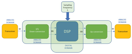
Figure 1.
System-level schematic of a generic RF channel emulator.
The system consists of a transmitter under test, a receiver and a channel emulation block having a number of key tasks to perform. The RF analog signal undergoes a down-conversion with the extraction of the in phase and quadrature components. The subsequent band-limited analog signal is sampled and processed in a specialized Digital Signal Processing unit (DSP) in order to introduce all the impairments typically present in a real propagation channel. These phenomena include the time-dependent attenuation, additive gaussian noise, jammers, Doppler spread and many others. The modified signal undergoes a digital-to-analog conversion and an up-conversion to be injected into the receiver. It has been investigated here with particular emphasis on the presence of time-variant delays due to a multipath propagation. Bearing in mind this aspect, with reference to Figure 1, the generic RF signal coming from the transceiver under test can be written as [2]
in which appear the envelope module , the instantaneous phase (t) of the modulating signal and the carrier angular frequency . The transit of the signal in Equation (1) through a delay line of seconds generates a new signal y(t) of the type:
The complex envelope of the signal in Equation (2), with respect to the angular frequency is equal to:
Equation (3) allows the processing of the signal in Equation (1) using directly its equivalent low frequency representation. When multipath is present, it can be correctly represented at complex envelope level as in Figure 2, where the complex envelope of the signal affected by multipath propagation is seen as the sum of the contributions coming from n discrete independent paths, each affected by a time-dependent delay and a time-dependent attenuation. The direct path is characterized by an absolute delay starting from the initial observation time. The remaining paths are affected not only by the main delay, but also by differential delays (small) with respect to the latter:
with
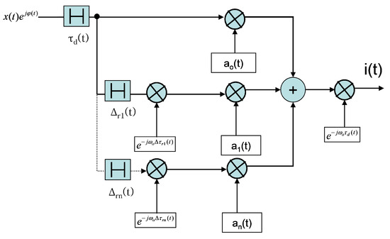
Figure 2.
Representation of the multipath signal in the complex envelope domain.
- equal to the distance (instantaneous) travelled by the direct path between transmitter and receiver;
- m/s equal to the speed of light;
- equal to the difference between the k-th path and the direct path.
By correctly emulating the behavior of the attenuations and the delays over time, the diagram in Figure 2 is able to correctly reproduce both fading and Doppler shift over the entire signal band, assuming the existence of a discrete number of independent paths [3]. In the perspective of a discrete-time realization, the scheme in Figure 3 considers the amplitudes and delays of each path as constants for sufficiently representative time intervals [4].
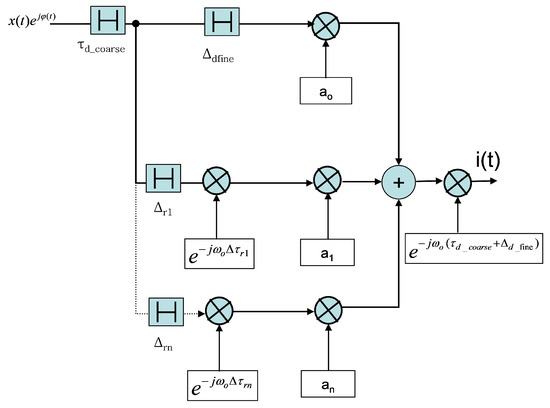
Figure 3.
Representation of the multipath signal in the complex envelope domain with delays and time-discrete amplitudes.
If we renounce to the complete emulation of the time-dependant delay of the direct path, losing therefore the absolute Doppler information, we arrive at the scheme in Figure 4.
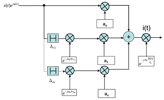
Figure 4.
Representation of the multipath signal in the complex envelope domain with delays and time-discrete amplitudes without absolute Doppler information.
In this last scheme, the Doppler shift is the one related to the frequency and depends directly on the law of variation of the direct path, with the addition of the spreading due to the variations of the delays of the reflected paths.
RF propagation in mobile channels is a very complex matter and several channel models have been developed, based on a statistical approach [5]. Narrowband channel emulators implementation have been proposed [6] and low-complexity architectures have been developed dealing with delays that are not integer multiples of the sampling rate [7] or solutions where massive calculations are demanded to a GPU (Graphical Processing Unit) using native highly parallelized architecture [8].
2.2. Required Sampling Step Size for the Emulation of the Effects of the Electromagnetic Propagation
Taking into account typical high speed vehicle dynamics and carrier frequencies (around few GHz), even with a simple two-rays model, the maximum expected Doppler shift is usually below few KHz. With reference to Figure 1, a correct emulation of the phenomenon performed by a DSP section requires a sampling step size of tens of microseconds (typically, ≤30 us). This is largely guaranteed by the sampling frequencies of the DSP sections that can run up to few GHz. To correctly emulate the multipath phenomenon, it is instead necessary that, during the minimum value of the differential delay of a path, the signal of the generic ray covers a space less than a fraction of the wavelength. The simple two-rays model allows some basic evaluations: for each differential delay , the spectral distance between two contiguous minima of the time-varying transfer function is approximately Hz. If the system bandwidth is B MHz, and the differential delay is expressed in , the number of in-band minima is therefore about equal to . The bandwidth of each minimum, evaluated at −10 dB compared to the maximum, is equal approximately to Hz.
The bandwidth associated to the minima of the transfer function, for some values of , is visible in Figure 5 and Figure 6.
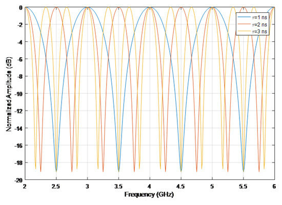
Figure 5.
Normalized amplitude transfer function for a two-ray model and different differential delays.
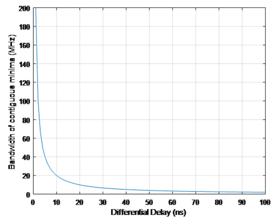
Figure 6.
Bandwidth in MHz at minima for a two-ray model.
Assuming a sampling frequency of 2 GHz for the DSP section and a corresponding sampling interval of 0.5 ns, in this interval the kth path covers about 0.15 m or up to 3 , for a RF spectrum from 2 to 6 GHz. Considering the phenomenon only in terms of RF propagation, it can be considered sufficient to limit the sampling frequency in order to have at least two samples per period or better.
2.3. Required Sampling Step Size for the Emulation of the Time Expansion
The emulation of the Doppler effect according to the principle of time expansion, performed digitally, implies a continuous discrete rotation of the signal phases in the different paths (see Figure 3) according to the time evolution of the respective delays. This entails an in-depth examination of what has already been discussed. To try to quantify the phenomenon, take into consideration the operation of quantization of the delay using a quantum equal to seconds:
The previous operation performs a uniform quantization of the original signal. For simplicity, we can imagine the following scenario: a fixed source transmits a pure tone at frequency f, a receiver moving at constant speed with a null initial distance, receives this signal with a variable delay :
The quantization of the delay generates a discrete signal so that the error
i.e., the difference between the original and the quantized one, normalized to , is limited to . The error pattern is a sawtooth signal with a period (see Figure 7).
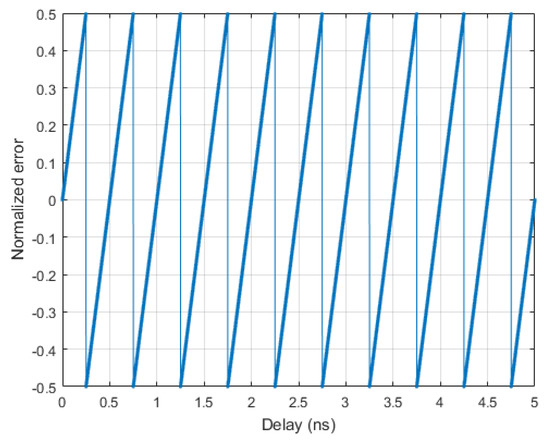
Figure 7.
Normalized quantization error.
The complex envelope of the received analog signal, with respect to the angular frequency , is:
Considering therefore the quantized delay, equal to , it is possible to calculate the complex envelope of the actual received signal obtaining:
The error signal is periodic, therefore it is possible to write it as a Fourier series expansion:
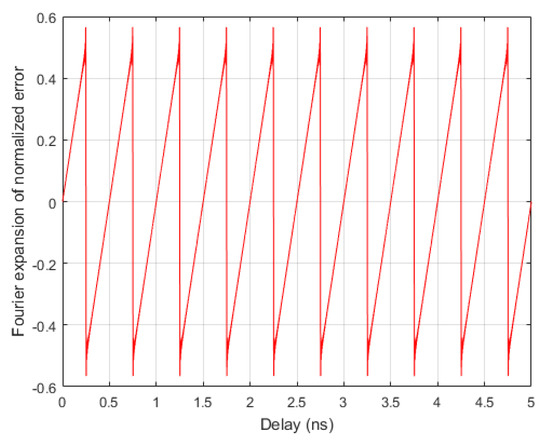
Figure 8.
Reconstructed error signal.
The complex envelope of the received signal thus results:
From Equation (11) it is evident how the quantization of the delay involves the generation of a non-linear phase modulation of the received signal. The associated real signal results:
The spurious phase modulation introduced may be neglected if . The time-dependent delay time, provided as input to the channel emulator, is still sampled at frequency even if no longer quantized. The signal received is therefore also sampled at this frequency. For a given platform speed, it is theoretically possible to eliminate unwanted components by imposing , resulting in a sampling of the sinusoidal component at integer multiples of the period. The complex envelope of the quantized signal can be placed in the form:
with a theoretically infinite number of products. Each complex exponential, with sinusoidal argument, can be placed in the form:
with equal to the Bessel function of order n of first kind. In first approximation, it can be sufficient to stop the series in Equation (12) considering only the orders and remembering that . Each summation in Equation (14) can then be put as follows:
thus obtaining:
by stopping the products at the third order, it is possible to write, for the real signal:
In addition to the expected tone, affected by a Doppler shift at frequency with an amplitude equal to , there are also spurious tones arranged symmetrically with respect to the central one. These components are separated by multiple integers of the frequency of the sawtooth wave with decreasing amplitudes.
3. Results
Defining the quantities:
the power ratio between the fundamental component and the first unwanted (nearest) spurious tone is:
With these assumptions it is possible to determine the equivalent sample step size required to generate the time-dependent delays while respecting a given spectral mask. This can be accomplished, for example, using fractional filters with a suitable resolution in order to obtain the required SLL as shown in Figure 9
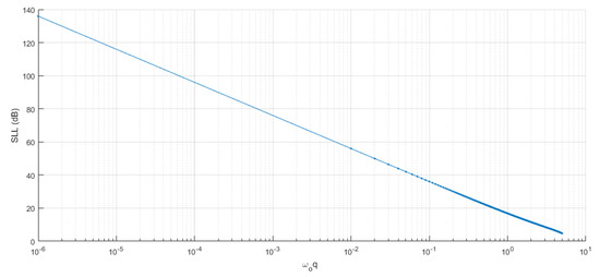
Figure 9.
SLL as a function of the product .
Figure 10 and Figure 11 show some Matlab simulations obtained with q = of the clock period and q = of the clock period, which confirm the expected spurious levels.
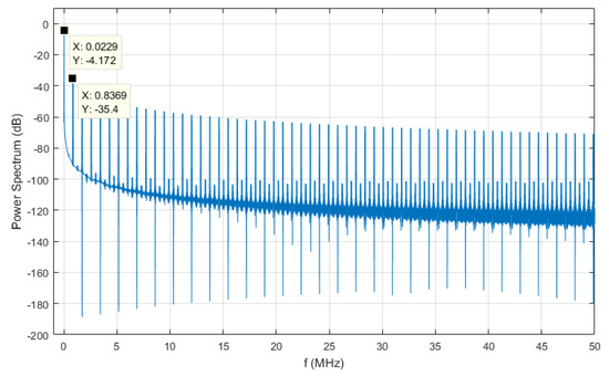
Figure 10.
Sidelobe level as a function of fractional quantum q = , spur @ 837 KHz, SLL∼ 32 dB.
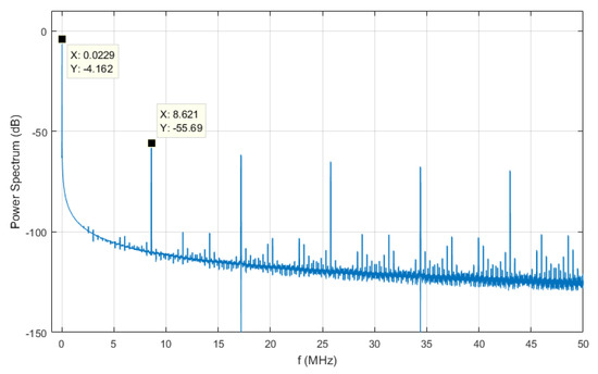
Figure 11.
Sidelobe level as a function of fractional quantum q = , spur @ 8.62 MHz, SLL∼ 51 dB.
4. Conclusions
In this paper, from a system level point of view, one of the numerous aspects of a real time RF channel emulator is analyzed. In particular, the sampling frequency required by a DSP section is investigated to correctly emulate the Doppler effect in a wideband RF signal using a general Time Expansion process without using artificial oscillators typical of narrowband channel models. The analysis allows determining the required sampling step size by the time-variant delays and to control, at the same time, the spectral purity of the emulated signal.
Funding
This research received no external funding.
Conflicts of Interest
The author declares no conflict of interest.
Abbreviations
The following abbreviations are used in this manuscript:
| UAV | Unmanned Aerial Vehicle |
| DEM | Digital Elevation Model |
| DSP | Digital Signal Processing |
| GPU | Graphical Processing Unit |
References
- Simon, M.; Alouini, M.S. Digital Communication over Fading: Channels A Unified Approach to Performance Analysis; John Wiley & Sons, Inc.: New York, NY, USA, 2000; pp. 15–28. ISBN 9780471317791. [Google Scholar]
- Sklar, B. Digital Communications: Fundamentals and Applications; Prentice Hall, Inc.: Upper Saddle River, NJ, USA, 2001. [Google Scholar]
- Boualleg, S.; Haraoubia, B. Influence of Multipath Radio Propagation on Wideband Channel Transmission. In Proceedings of the International Multi-Conference on Systems, Signals & Devices, Chemnitz, Germany, 20–23 March 2012. [Google Scholar] [CrossRef]
- Oppenheim, A.V.; Schafer, R.W. Discrete-Time Signal Processing; Prentice Hall, Inc.: Upper Saddle River, NJ, USA, 1999. [Google Scholar]
- Patzold, M. Mobile Fading Channels; John Wiley & Sons, Ltd.: West Sussex, UK, 2002; pp. 289–320. ISBN 0-471-49549-2. [Google Scholar]
- Green, P.J. Implementation of a Real-Time Rayleigh, Rician and AWGN Multipath Channel Emulator. In Proceedings of the 2017 IEEE Region 10 Conference (TENCON 2017), Penang, Malaysia, 5–8 November 2017; pp. 35–39. [Google Scholar]
- Hofer, M.; Xu, Z.; Zemen, T. Real-time channel emulation of a geometry-based stochastic channel model on a SDR platform. In Proceedings of the 2017 IEEE 18th International Workshop on Signal Processing Advances in Wireless Communications (SPAWC), Sapporo, Japan, 3–6 July 2017. [Google Scholar]
- Alvarez, R.C.; Castillo, J.V.; Atoche, A.C.; Aguilar, J.O. A fading channel simulator implementation based on GPUcomputing techniques. Math. Probl. Eng. 2015, 2015, 237061. [Google Scholar]
© 2019 by the author. Licensee MDPI, Basel, Switzerland. This article is an open access article distributed under the terms and conditions of the Creative Commons Attribution (CC BY) license (http://creativecommons.org/licenses/by/4.0/).