
Development of an Optical System for Non-Contact Type Measurement of Heart Rate and Heart Rate Variability

Department of Electrical Engineering, Veermata Jeejabai Technological Institute (VJTI), Mumbai 400019, India
*
Author to whom correspondence should be addressed.
Appl. Syst. Innov. 2021, 4(3), 48; https://doi.org/10.3390/asi4030048
Submission received: 16 June 2021
/
Revised: 22 July 2021
/
Accepted: 23 July 2021
/
Published: 28 July 2021
Abstract
:Self-mixing optical coherent detection is a non-contact measurement technique which provides accurate information about the vibration frequency of any test subject. In this research, novel designs of optical homodyne and heterodyne detection techniques are explained. Homodyne and heterodyne setups are used for measuring the frequency of the modulated optical signal. This technique works on the principle of the optical interferometer, which provides a coherent detection of two self-mixing beams. In the optical homodyne technique, one of the two beams receives direct modulation from the vibration frequency of the test subject. In the optical heterodyne detection technique, one of the two optical beams is subjected to modulation by an acousto-optics modulator before becoming further modulated by the vibration frequency of the test subject. These two optical signals form an interference pattern that contains the information of the vibration frequency. The measurement of cardiovascular signals, such as heart rate and heart rate variability, are performed with both homodyne and heterodyne techniques. The optical coherent detection technique provides a high accuracy for the measurement of heart period and heart rate variability. The vibrocardiogram output obtained from both techniques are compared for different heart rate values. Results obtained from both optical homodyne and heterodyne detection techniques are compared and found to be within 1% of deviation value. The results obtained from both the optical techniques have a deviation of less than 1 beat per minute from their corresponding ECG values.
1. Introduction
The maximum critical cases across the world are related to chronic cardiorespiratory conditions. Demographic changes are expected to cause home monitoring approaches to take a leading role in the future treatment of such patients [1,2]. Remote monitoring technologies have gained a significant importance in the COVID-19 era. During the pandemic, the use of non-contact type techniques for the measurement of bio-parameters have increased rapidly. Although fixed-on-body electrodes are reliable and give good signal quality, there are several disadvantages of this method. The major demerit of this technique is the direct fixing of electrodes on skin, as it leads to discomfort among patients. Direct measurement on skin becomes very critical, especially in the case of infants and people with burn injuries. Therefore, the interpretation of cardiovascular signals through unobtrusive means has gained importance in recent years. A vast amount of research is available for the measurement of cardiovascular parameters, but most of the research is related to contact type measurement. There is much less clinical awareness of non-contact type optical measurement of cardiovascular parameters. There are several reasons contributing to this fact, such as the absence of a specific therapy for prognosis improvement. Furthermore, there is a lack of standardized methodology for parameter assessment due to the variability of factors, such as gender, age, medical history for illness, and drug interferences [3]. The common intention behind this development is to enable the monitoring of cardiovascular parameters, such as heart rate (HR) and heart rate variability (HRV), in scenarios that prevent the use of conventional clinical sensors, normally requiring some sort of direct electrical (resistive) or mechanical coupling. Less variation in HR is not good for the health of a person. Generally, a high variability in HR is an indicator of good health for a person [4,5]. HRV provides information about the person’s physical and emotional response towards any illness and stress [6]. It can provide important information about blood sugar, blood pressure, digestion, and the respiration cycle. Understanding HRV provides vital information about many biological systems and processes. The measurement of HRV is more complex than the measurement of HR. As HRV measurement involves changes in the heart period in the order of milliseconds, it requires higher degrees of accuracy than HR.
Optical interferometer-based detection setups are widely used in many fields, such as medicine, automation, and architecture. Optical coherent detection techniques mainly consist of homodyne and heterodyne type detection methods. S.F. Jacobs first provided the theoretical comparisons of two detection schemes [7], compared the modulation schemes of both techniques, and provided the methods of optical beating inside a Mach–Zehnder interferometer. Koukoulas et. al. presented the results of a hydrophone calibration comparison between reciprocity and interferometry [8]. The same author provided a comparison between heterodyne and homodyne interferometry in order to realize the acoustic pascal unit of acoustic pressure in water [9]. The author directly compared the two techniques used in underwater acoustics and ultrasonics in terms of acoustic pressure estimation.
More recently, laser vibrometers have been considered for the non-contact monitoring of cardiac activity from measurements performed on the chest wall. Laser Doppler vibrometer-based methods are used to perform both HR and HRV analysis, with results equivalent to ECG. Tomasini et al. demonstrated the measurement of pressure waves by means of a laser vibrometer [10]. Morbiducci U et al. used a commercial laser Doppler vibrometer for vibratory measurements at long operative distances (tens of meters) [11,12]. Lorenzo Scalise et al. proposed a protocol for monitoring cardiac activity by measuring the skin surface vibrations of the main neck vessels caused by vascular wall motion in the carotid artery [13]. The author proposed the measurement of the velocity of displacement of the skin in correspondence to the chest wall. The method is based on the optical recording of the movements of the neck by means of laser Doppler interferometry. De Melis et al. proposed a vibratory signal measurement from the chest wall and carotid [14]. Many studies have demonstrated displacement measurements with (or better resolution). In this approach, scattered light from a vibrating surface is used to detect the amplitude and frequency of surface vibrations [15,16,17]. Many studies have demonstrated the absolute distance measurement with a self-mixing method [18,19,20,21,22].
The heart and lungs work together to transport oxygenated blood throughout the body. Deformation of the heart results in the generation of vibration frequencies on human skin, especially on the chest wall and the wrist. Therefore, the analysis of vibrations on the skin surface provides crucial information about the type of disorder. The movement and deformation of the heart, as well as the pulse wave traveling through the body, results in displacement and vibration of the body surface [23]. The human chest wall consists of independent mechanical components that contribute to chest wall mechanics. Optical coherent detection is one of the important techniques for measuring the frequency of vibration on a test subject. The aim of the optical sensing method proposed here is to observe the activity of the heart with an approach based on a custom-made low-cost self-mixing laser interferometer. The optical interferometer-based system directly measures the vibration frequency on human skin with a very high accuracy and temporal resolution. The coherent detection technique involves the vibration measurement by two independent optical setups, namely homodyne and heterodyne. It works on the principle of the modulation of light signal by mechanical vibrations. Measurements carried out with these techniques are non-intrusive and non-destructive. These techniques are completely contactless and are relatively precise and sensitive [24]. The detection method is called self-mixing because the two interfering beams are obtained from the same optical source from the beam splitter [25]. The optical coherent detection technique is useful for the monitoring of the burnt patients or preterm infants.
The main contributions of this research are:
- A novel design of a self-mixing optical homodyne and heterodyne detection setup for measuring the vibrations of chest wall or wrist position is proposed;
- A comparison of results of homodyne and heterodyne techniques with available contact type measurement techniques, such as an electrocardiogram (ECG), is studied;
- The feature extraction of the vibrocardiogram (VCG) signal for the monitoring of HR and HRV is obtained.
In this research paper, Section 2 describes the modulation scheme for the design of optical homodyne detection and optical heterodyne detection. Section 3 provides details about the experimental setup for the measurement of vibration on the chest wall and wrist. Section 4 analyses the results of the HR and HRV measurement. In this section, feature extraction of vibrocardiogram (VCG) waves is performed and its mapping with ECG signal is explained. Further, the results of optical homodyne and heterodyne techniques are compared based on the results. The research also provides details of the construction of the proposed optical homodyne and heterodyne setups.
2. Optical Coherent Detection Technique
The optical coherent detection techniques consist of a Mach–Zehnder interferometer or Michelson interferometer. In a Mach–Zehnder interferometer, an optical signal is divided into two parts with a beam splitter. These two beams travel a distance of and in two orthogonal arms of the interferometer and are combined at another beam coupler, as shown in Figure 1. The two signals are made to travel exact equal distances, so that the total path difference between these beams is always zero.
Mirrors M1 and M2 are used to fine tune the total path difference between the two beams. Once the path difference (i.e., ) is zero, the phase difference between the two beams becomes constant or zero, as the phase difference is directly proportional to the path difference [26]. The interference pattern is observed at the photo detector. The phase difference (in radians) between the two beams is given by,
If the two beams travel an equal path, the path difference between them will be either zero or constant. It will lead to a constant phase difference between the two beams [27]. The condition for constructive interference is given by,
The condition of destructive interference is given by,
2.1. Optical Homodyne Detection
Even the well-behaved lasers, such as the Nd:YAG laser and He: Ne laser, show frequency fluctuations due to thermal change and vibrations. One solution for this problem is to use the same laser for the local oscillator and the signal beams. This type of system is called a “homodyne” system. The main advantage of this system is its insensitivity towards frequency fluctuations when the path length of the two arms are equal. The optical homodyne detection technique requires interference of the two optical beams. The first beam is the input optical carrier signal with frequency while the second optical beam is provided by a local oscillator with frequency as shown in Figure 2. The optical signal is demodulated directly to the baseband. It requires a local oscillator whose frequency matches the carrier signal and whose phase is locked to the incoming signal (). Information can be transmitted through amplitude, phase, or frequency modulation [28].
The input carrier signal is given by,
and the local oscillator signal is given by,
The output power of the photodetector is,
and the power of the modulated signal is given by,
while the power of the local oscillator signal is given by,
The intermediate frequency signal is given by , which is the difference of the carrier signal and local oscillator signal frequency.
The overall phase shift observed at the detector is the difference of the phase of input carrier signal and the local oscillator signal. The overall phase shift is given by,
2.2. Heart Rate Detection with Self-Mixing Optical Homodyne Technique
The optical homodyne detection technique for HR detection makes use of self-mixing of the same type of frequency signal, as shown in Figure 3. The laser diode signal with frequency is split in two orthogonal arms of a Michelson interferometer by a 3 dB beam splitter. The frequency of the optical signal remains the same in both orthogonal arms. In this case, the local oscillator signal is provided by a fixed mirror M, which reflects back the same optical signal, whose frequency is . The modulated optical signal is the optical signal that is reflected from the skin surface of the human test subject. Both the local oscillator and modulated signals are obtained in two orthogonal arms of the Michelson interferometer. Optical signals travel in the two orthogonal arms and are combined at the same 3 dB splitter. In this case, both optical signals travel the same path distance in the two arms of the interferometer.
Thus, the total path difference in the two orthogonal arms becomes zero. The zero-path difference in both orthogonal arms leads to zero phase difference between two optical signals. Therefore, the phase of the carrier signal with frequency is matched to the local oscillator signal with frequency and the phase of both the beams are locked [29]. The Modulated bio signal is given by,
The local oscillator signal is given by,
The output power of the photodetector is,
The intermediate frequency signal is given by , which is the difference of the carrier signal and the local oscillator signal frequency.
The beating of the two optical signals provides the HR frequency () at the photo detector, which is equal to , i.e.,
The overall phase shift observed at the detector is the difference of phase of modulating bio signal () and phase of input optical signal (). It is given as,
The phase difference between both orthogonal beams is zero and constant inside the interferometer.
2.3. Optical Heterodyne Detection Technique
The optical heterodyne detection scheme consists of acousto-optic modulators (AOM) in order to generate an optical frequency shift. An acousto-optic effect is generated with an acoustic wave into a lead molybdate crystal. The acoustic wave causes a change in the refractive index, which is periodic in nature. This generates an effect analogous to a moving diffraction grating along the material, with the site spacing equal to the wavelength of the acoustic wave. An AOM cell, as shown in Figure 4, is constructed using a piezo-electric transducer to introduce the sound waves into the transparent material. It creates a diffraction grating in the material which has a spacing equal to the order of the wavelength of the acoustic wave. A piezo-electric transducer is used to create the acoustic wave into the lead molybdate crystal. In AOM, the angle of incidence satisfies Bragg’s condition for constructive interference. The period of spacing created by the acoustic wave is given by . In order to satisfy Bragg’s condition, the incident angle () is given by,
The optical heterodyne technique makes use of modulation from the AOM frequency signal, as shown in Figure 5. The input signal with frequency is combined with the local oscillator signal with frequency by using a 3 dB beam combiner. The combined frequency of the optical signal remains the same () in both orthogonal arms. The AOM modulates the optical signal in one arm with modulation frequency . The optical beating of one signal with frequency and the other signal with frequency will result in the direct detection of modulation frequency at the photo receiver [30].
2.4. Heart Rate Detection with Self Mixing Optical Heterodyne Technique
The self mixing interferometer consists of a Mach–Zehnder interferometer, as shown in Figure 6. Unlike homodyne detection, the frequency of the fundamental optical signal is not same as the local oscillator signal ( in heterodyne detection. Therefore, the modulation frequency is detected at the receiver due to optical beating. The self-mixing optical heterodyne detection technique makes use of AOM in the test arm of the interferometer.
Figure 7 shows the detection of the HR signal with the self-mixing heterodyne detection scheme. The test arm of the Mach–Zehnder interferometer consists of an AOM. The optical signal first becomes modulated by the RF frequency given to the AOM. Further, this signal is subjected to another modulation by reflection from the chest wall of the test subject. The chest wall vibrations are due to the HR frequency . The optical signal after reflection from the chest wall has a frequency of The fundamental optical signal passes through the reference arm of interferometer. The fundamental optical signal and bio-modulated optical signal orthogonally combine at the 3 dB coupler. In this case, in both arms of the interferometer, optical signals travel the same path distance. The total path difference in the two orthogonal arms becomes zero. The zero-path difference in both orthogonal arms leads to a zero phase difference between the two signals. Therefore, the phase of the modulated signal with frequency is matched to local oscillator signal with frequency and the phase of both the beams are locked [31].
The modulated bio signal in the test arm of the interferometer is given by,
The fundamental optical signal in the reference arm of the interferometer is given by
The output power of the photodetector is given by,
The intermediate frequency signal is given by , which is the difference between the frequency of the test and the reference signals.
provides the heart frequency with the modulation frequency of AOM at the photo detector,
The overall phase shift observed at the detector is the phase difference of the modulating signal in the test arm and the fundamental signal in the reference arm [32]
3. Experimental Setup of Optical Homodyne and Heterodyne Detection
3.1. Experiment for Heart Rate Detection with Self-Mixing Optical Homodyne Technique
Thin nano film reflectors are used for reflection of the laser signal. These reflectors are mounted on the wrist and chest wall of the test subject. Due to their negligible mass, thin film reflectors vibrate with the same frequency as that of heart frequency. The thin film reflectors are prepared with gold sputtering and aluminum sputtering techniques. Thin antireflection coating on glass for optical applications are deposited by sputtering. Sputtering is a vapor phase deposition (PVD) method of thin film deposition [33]. This involves ejecting material from source onto a silicon wafer. Optical coatings are deposited in the wavelength regions between visible and far-IR. The used samples were silica substrates with thickness of 1 μm. The atomic force microscopy (AFM) image of gold-sputtered thin film nano reflector is shown in Figure 8. In order to optimize the quality of the bio-signal, a thin film reflector with an adhesive tape was placed on the chest wall. The thin film reflector increases the S/N ratio of the vibratory signal. Instead of thin film reflectors, 45% hydrating zinc oxide spray or paste on skin can also be used in order to maximize the reflection.
The experiment setup of homodyne detection consisted of a laser diode, a beam splitter, mirrors, and photodetectors. The laser diode used in this setup was semiconductor AlGaInP laser with wavelength 660 nm and power 10 mW. The laser beam is split into two parts by a beam splitter. One beam travels towards the fixed mirror while other beam travels towards thin film reflector, which is fixed on the human wrist or the chest wall. Both beams after reflection from the mirrors combine at the same beam splitter and interference pattern is observed at the photodetector. A tight strip band is fixed near the elbow position so that heart pulse is properly located on the wrist. Figure 9 shows the experimental setup for homodyne detection scheme. Figure 10 shows the response of photodetector for homodyne detection. It clearly shows measurement of vibration on human wrist skin, which indicates heart frequency. The measurement of heart frequency was carried out at the chest wall position with similar results. The laser was placed at approximately 10 cm from the subject’s chest wall and wrist position [34]. A low pass filter (cut off frequency Hz) was placed in series with photo detector for denoising of the optical beat signal. Laser diode with power of 10 mW was used, so that no special safety measures were required. Even with low power level, a working distance of 10 m is feasible.
3.2. Experiment of Heart Rate Detection with Self Mixing Optical Heterodyne Technique
The AOM used for this experiment was ISOMET AOM with model number 1205C-2 [35]. Table 1 shows the specifications of ISOMET AOM.
An RF signal source was used to modulate the reference frequency of the actual laser beam. RF signal generator tunes the laser beam given to AOM and modulates it with various frequency range. Further, an RF amplifier was used in series with RF generator to provide high gain. RF amplifier was needed because AOM requires a minimum 25 dBm RF power as an input in order to provide modulation. The maximum gain of 32 dB can be obtained with RF amplifier. Table 2 shows the specifications of the RF generator and the RF amplifier circuit.
The optical signal produced multiple order side bands with frequency . These side bands are shown in Figure 11a,b. Figure 12 shows the modulation of 660 nm laser beam with 60 MHz RF signal, where 660 nm laser corresponds to 454.5 THz frequency. Light signal was modulated by the RF signal of 60 MHz after passing through AOM [36].
Figure 13a,b shows the optical heterodyne detection setup and measurement of heart frequency at the wrist position of the test subject, respectively. The optical signal is divided into two parts with beam splitter. One part of the optical signal travels in test arm of interferometer which consists of an AOM, while the other part of the optical signal travels in the reference arm of the interferometer. The bio-modulated optical signal reflected from the subject is combined with AOM modulated optical signal at a beam splitter in the test arm. The optical beat signal of test arm and reference arm is obtained at the 3 dB coupler. The measurement procedure on human skin for optical heterodyne detection was the same as that of the optical homodyne detection setup.
Figure 14 shows the response of the photodetector for intermediate frequency . Figure 15 shows the detection of heart frequency . The heart frequency was obtained by demodulation of intermediate frequency with modulation frequency . A frequency mixer was used for the purpose of demodulation and extraction of heart frequency from intermediate frequency.
4. Measurement Results of HR and HRV with Optical Homodyne and Heterodyne Technique
HR is measured in average beats per minute, while HRV measures the specific changes in time between successive heart beats. A low HR indicates rest, while a high HR corresponds with physical exertion. The interbeat interval or heart period (HP) is the time between successive heart beats.
4.1. Recording of Vibrocardiogram and Electrocardiogram Signal
It is equally important to compare a non-contact type optical detection method with existing contact type measurement methods, such as ECG. The commercially available AD8232 chip, designed for ultra-low power applications, is used as a contact type sensor for a results comparison with an accuracy of more than 96% [37,38]. AD8232 is used in a three electrode configuration and makes use of right arm (RA), left arm (LA), and right leg (RL) electrodes to acquire bio-potential signal. It has the capability to acquire, amplify, and filter bio-potential signals. This chip is capable of eliminating the motion artifacts and the electrode half-cell potential. The output obtained from the AD8232 module is processed with a microcontroller. The standard PQRST waveform signal is obtained with it. The successive R-R interval in milliseconds is calculated for the HR measurement. The detrending and denoising of the raw ECG signal is performed by wavelet analysis. The equation to calculate HR in beats per minute is given as,
The optical beat signal obtained from the coherent detection is called a vibrocardiogram (VCG), as the light signal is modulated by vibrations from the chest wall or wrist. On each individual measurement, the ECG and VCG traces were simultaneously recorded. Figure 16, Figure 17, Figure 18, Figure 19, Figure 20, Figure 21 and Figure 22 shows the detection of the HR with optical sensing. Short-term recordings (5 min) were carried out on 20 human subjects (ten males aged from 20 to 40 years; ten females aged from 20 to 40 years). All the participants signed an informed consent agreement before taking part in the tests. The HR per minute is measured for a different set of test subjects, with varying physical activities, such as running, walking, speaking, and resting [39]. The ECG and VCG data are recorded for multiple human subjects and are mainly divided into three categories (resting, active, and exertion). Table 3 shows information about the subjects under test.
For the HR measurement of physical exertion, the test subjects were asked to go through excessive physical activities, such as climbing stairs or exercise, just before the measurement. Physical exertion leads to artifacts in the measurement on the test subject. These artifacts are basically associated with a high respiration rate, which causes rapid change in the chest wall motion. Frequent motion of the chest wall leads to shift in the baseline of the VCG signal. The motion artifacts associated with respiration are always present in the HR signal in the form of baseline wandering. The baseline drift is removed by denoising and detrending. Figure 23 shows the VCG signal for 72 bpm, 90 bpm, and 102 bpm with the same time axis. From Figure 23, the VCG signals with different HR can be identified easily.
4.2. Feature Extraction in VCG and Its Mapping with ECG
The oxygen-rich blood returns from the lungs and flows into the heart’s upper left atrium. The oxygen-depleted blood returns from the rest of the body and flows into the right atrium. Both the left and the right atria become filled with blood. The sinus node (SA) in the right atrium produces a small electrical pulse. The systole and diastole are the two processes that are associated with the period of contraction and relaxation of the heart, respectively. The electrical pulse causes the heart contraction. Due to this, mechanical vibrations are originated and propagate through different tissue layers before being detected on the skin with an optical sensing technique [40]. The factors which influence the vibration signal are the time and amplitude characteristics of the electrical pulse and the mechanical response of the heart. These factors depend on specific characteristics, such as body mass index (BMI) and the medical history for the disease. It is important to map the electrical activity of the heart with its mechanical response, as it provides useful information about the activity of the heart. In the following section, the mapping of ECG and VCG is performed, and its significance is explained.
- 1.
- P wave: The P wave represents the depolarization of the left and right atrium. It corresponds to atrial contraction. The point of local maximum in the ECG for the P wave corresponds to the point of the first local minima in the VCG, as shown in Figure 24. The opposite nature of the electrical and mechanical signal is due to atrial contractions [41];
- 2.
- PR interval: During the PR interval, the electrical pulse moves from atria to ventricles. The PR interval in the ECG has a duration of approximately 120–200 ms. The contractions of ventricles generate vibration patterns that are observable in the VCG plot. When the ventricle contracts, a dominant negative deflection is generated. Thus, it is possible to distinguish between a heartbeat and a beat drop. The atrial contractions result in positive deflections. The PR interval in the ECG is mapped to the interval between the first local minima and the second zero crossing of the VCG signal;
- 3.
- QRS complex: The point Q in the ECG corresponds to the point of first local maximum , while the point of minimum S in the ECG corresponds to the point of second local minima in the vibrocardiogram signal, as shown in Figure 25. The R wave in the ECG corresponds to the zero crossing of the VCG signal [42]. The zero crossing is a point which is located at the center of and . It is located exactly at the center of the first maxima and the second minima of the VCG signal.
The total time duration of the QRS signal represents the depolarization of ventricles. During this time interval, the chest wall vibration reduces significantly from maximum to minimum;
- 4.
- ST segment: The T wave represents ventricular repolarization. It appears as a small wave after the QRS complex. The ST segment starts at the end of the S wave and ends at the beginning of the T wave. The ST segment is an isoelectric line that represents the time between depolarization and repolarization of the ventricles. The T wave in the ECG corresponds to the wave of the VCG, as shown in Figure 26;
- 5.
- QT interval: The QT interval begins at the start of the QRS complex and finishes at the end of the T wave. The QT interval in the ECG is mapped to the interval of the VCG. It represents the time taken for the ventricles to depolarize and then repolarize [43].
The complete VCG cycle is mapped to the ECG cycle for the heart period (HP). Figure 27 shows the significance of features in the VCG with reference to the ECG. From the recordings of both the signals, the relationship between the ECG to the vibratory signal VCG in terms of heart rate variations is analyzed. The peak vibratory signal is due to chest wall motion. This signal is generated due to cardiac muscle contraction triggered by the electrical signal. The first local maximum value is labeled as in the VCG, while the first local maximum in the ECG curve is labeled as R. For the measurement of HR and HRV, V-V interval () is considered, and this measurement is compared with the R-R interval () in the ECG trace [44]. By using Equation (23), the HR can be calculated from the VCG signal as,
4.3. Measurement of HRV
The time difference between two successive R peaks is calculated throughout the ECG wave. The mean value of this time difference is called the R period. Similarly, the time difference between two successive peaks is calculated, and this time difference is called the V period. The R period and V period provide the time duration for each heart activity. The difference between two consecutive R period intervals is calculated as the R-R variability, while the difference between two consecutive V period intervals is calculated as the V-V variability [45]. In this experiment, different subjects with different ages and BMI are considered. Table 4 shows an example of the measurement of the heart period and HRV by means of ECG and VCG waveforms. For this measurement, the test subject was in a state of rest. In order to measure the HRV, the periodic characteristic related to the heartbeat needs to be identified [46].
From Table 4, the mean value of the R-R interval is calculated to be 101.056 ms with a standard deviation of 48.8 ms and a standard error value of 6 ms, while the mean value of the V-V interval is calculated to be 101.257 ms with a standard deviation of 36.3 ms and a standard error of 4 ms. The UU variability and VV variability are equal, as they are part of the same signal. Therefore, for further analysis of HRV, only one of UU or VV variability is considered.
Figure 28 shows the column chart representation of variability in the R-R interval, U-U interval, and V-V interval, simultaneously. The heart period for each heartbeat count for both the ECG and VCG signal is represented as a vertical column line. For the VCG signal, the heart interval is measured for both the U-U and V-V wave, while the R-R wave is considered for the ECG [47]. From Figure 26, it is clear that the measurement of HRV from the ECG and VCG plots shows similar results, with a less than 1% deviation value. Figure 29 and Figure 30 show the R-R and V-V variability plot for the test subject under sleep. A HR of 40 bpm is measured with the test subject under deep sleep. Figure 31 shows HRV analysis of the test subject under an active state, and a HR of 72 bpm is measured. Figure 32 and Figure 33 show HRV analysis of the test subject under excessive stress and physical exertion, respectively. A HR of 96 bpm and 108 bpm are recorded for test subjects under excessive stress and physical exertion, respectively. All results shown here are obtained on the chest wall. Figure 34 shows the HRV in the ECG and VCG for different test subjects. The measurement of HRV from the VCG shows much less deviation from their corresponding ECG values.
Table 5 shows a complete summary of HR and HRV for different test subjects under deep sleep, active state, and excessive exertion. It is clear that the ECG recording and VCG recording show similar results for HRV and HR. For non-contact type measurement, both homodyne and heterodyne detection techniques are used. The HR and HRV values obtained from homodyne and heterodyne detection show much less deviation from the ECG values.
4.4. Comparison of Results of Optical Homodyne and Heterodyne Technique
The accuracy of heterodyne detection is found to be better than homodyne detection. The use of AOM in heterodyne detection limits the noise associated with the laser oscillator. However, both optical coherent detection techniques show much less deviation from the ECG recording. Table 6 shows a comparison of results obtained from homodyne detection and heterodyne detection and their deviation from the ECG results. The mean deviation between the electrical measurement and optical measurement methods for each subject is reported [48,49,50] and computed with the equation,
A small value of deviation from the ECG proves that the VCG graph provides an accurate measurement of HR and HRV. As shown in Table 6, the deviation values between the VCG and ECG approaches zero for a measurement of HR lower than 70 bpm. For a measurement of HR higher than 70 bpm, the deviation values are less than 0.5. The measurement of higher HR is associated with many factors, such as medical history and the psychological and emotional behavior of the subject under test.
Table 6 clearly shows that HR values obtained from both techniques are very close to HR values obtained from the ECG recording. The obtained results are motivating because optical detection is a completely non-contact type measurement technique. Table 7 shows the values of HR obtained from the coronary artery (chest wall position) and radial artery (wrist position) of two test subjects. The measurement of HR at the coronary artery and radial artery shows very little deviation, at less than 1 bpm.
Figure 35a,b shows a comparison of homodyne and heterodyne techniques for the measurement of a HR of 54 bpm and 84 bpm, respectively. It is clear from Figure 35a that homodyne and heterodyne detection show identical results for measurement associated with the lower value of HR. Figure 36b shows a deviation of 0.22 bpm when measuring the higher value of HR. The measurement of deviation of the VCG values from ECG values are performed for both homodyne and heterodyne techniques. Figure 36a,b shows the mapping of the heterodyne and homodyne signal with the ECG signal for a HR of more than 70 bpm, respectively. Figure 36a shows that the R peak of the ECG precisely maps to the zero crossing between the point and point in the VCG associated with the heterodyne measurement system. Figure 36b shows that there is a small delay between the R peak of the ECG and the zero crossing between the point and point in the VCG associated with the homodyne measurement system. These results show that for measurement of a higher value of HR, optical heterodyne measurement provides better accuracy compared to optical homodyne measurement. The delay approaches to zero for the heterodyne measurement system. However, the delay measured for homodyne detection is found to be less than 3 ms. The delay leads to a maximum deviation of around 0.5 bpm from the ECG values. Thus, measurements recorded with the optical homodyne setup are comparable with both the optical heterodyne and ECG setup. The deviation values from the ECG are found to be less than 1%. Figure 37 shows the deviation of both techniques from the ECG values. Figure 38a,b shows the distribution of the deviations in bpm for the case of chest wall measurement (subject 7). The histogram is fitted with a Gaussian distribution, with a mean value of 0.04 bpm and a standard deviation of 1.1 bpm for heterodyne detection. The histogram is fitted with a Gaussian distribution mean value of 0.06 bpm and a standard deviation of 1.6 bpm for homodyne detection. The value of uncertainty calculated with the heterodyne detection method is bpm, while for the homodyne detection method, the value of uncertainty is calculated as bpm.
5. Discussion
Self-mixing optical coherent detection is an important sensing method for the assessment of cardiac, respiratory, and muscular activities. HRV is an important parameter to analyze both the overall health and the ability to tolerate stress [51]. Optical coherent detection techniques have the advantage of being a contactless method, as it becomes very helpful in measurements from critically damaged skin conditions. They are also useful for measurements on the delicate skin of preterm infants. HP can be measured by detecting a periodic feature in the waveform acquired, such as and peaks in the VCG signal. A comparison of R peaks in the ECG with V peaks in the VCG signal was performed and both the measurements were found to be similar, with a less than 1% deviation. The mapping of features of the ECG signal is performed with VCG signal features [52]. In this research paper, measurement results from homodyne and heterodyne techniques are compared with the ECG signal. In future, the accuracy of homodyne and heterodyne measurements can be compared with other signals of a different nature, such as the photoplethysmograph (PPG) and phonocardiogram (PCG). The ECG is the electrical signal, which is a representation of the electrical response of the heart activity. The PCG is the audio signal and represents the acoustic response of the heart activity. The PPG is the optical signal, while the VCG is the mechanical signal. During an arrhythmia, the heart can beat too fast, too slowly, or with an irregular rhythm. The first-degree AV block occurs when the PR interval is more than 200 ms. The AV block can be easily correlated with the VCG signal when there is a delay between and the zero crossing of the VCG signal [53]. The stability of coherent detection can be improved by the construction of a multiple mirror Fabry–Perot resonator in one of the arms of the interferometer, or by implementing a servo motor mechanism for the motion of mirrors [54,55,56,57,58].
6. Conclusions
In this research, a novel design of optical homodyne and optical heterodyne detection is explained. The optical homodyne technique consists of a simple setup, but the optical heterodyne technique makes use of complex optical components, such as AOM. The optical homodyne detection makes use of the direct modulation of the fundamental optical signal, while the optical heterodyne detection technique makes use of the modulation of the higher order mode of the optical signal. The path length fluctuations are the main problem in optical homodyne detection. The phase fluctuations related to the path length difference can have very little variation in a homodyne setup. This problem can be solved with optical heterodyne detection, as the frequency of the local oscillator is not equal to the signal frequency in optical heterodyne detection . In case of measurement of high values of HR (more than 70 bpm), the optical heterodyne detection has a higher accuracy of results compared to optical homodyne detection. This is due to the fact that variation in the path length difference is very limited in the homodyne setup ( However, results obtained from the homodyne method show much less deviation from results of the heterodyne setup and ECG setup. The deviation of results is less than 3 ms for measurement of the heart period and less than 0.5 bpm for measurement of the HR. Both homodyne and heterodyne detection techniques can be used to accurately measure HR and HRV. The experimental results of homodyne and heterodyne detection are comparable with contact type measurement methods, such as an ECG. The results are found to be within a less than 1% deviation value from the ECG measurement.
Author Contributions
J.G. performed the conceptualization, methodology, software, validation, formal analysis, and investigation. M.S.P. performed the supervision and project administration. The writing, review, editing, and visualization are carried out by J.G. All authors have read and agreed to the published version of the manuscript.
Funding
This research received no external funding.
Informed Consent Statement
Informed consent was obtained from all subjects involved in the study.
Data Availability Statement
The data presented in this study are available on request from the corresponding author. The data are not publicly available due to privacy issues.
Acknowledgments
We would like to acknowledge Arpit Rawankar, Visiting Fellow from Tata Institute of Fundamental Research, Mumbai, India for providing optical components used for the experiment.
Conflicts of Interest
The authors declare no conflict of interest.
References
- Tanzi, L.; Vezzetti, E.; Moreno, R.; Aprato, A.; Audisio, A.; Massè, A. Hierarchical fracture classification of proximal femur X-Ray images using a multi-stage deep learning approach. Eur. J. Radiol. 2020, 133, 109373. [Google Scholar] [CrossRef]
- El-Saadawy, H.; Tantawi, M.; Shedeed, H.A.; Tolba, M.F. Deep Learning Method for Bone Abnormality Detection Using Multi-View X-rays, International Conference on Artificial Intelligence and Computer Vision; Springer: Cham, Switzerland, 2021; pp. 46–55. [Google Scholar]
- Schroeder, E.B.; Liao, D.; Chambless, L.E.; Prineas, R.J.; Evans, G.W.; Heiss, G. Hypertension, Blood Pressure, and Heart Rate Variability. Hypertension 2003, 42, 1106–1111. [Google Scholar] [CrossRef] [PubMed] [Green Version]
- Mejía-Mejía, E.; Budidha, K.; Abay, T.Y.; May, J.M.; Kyriacou, P.A. Heart Rate Variability (HRV) and Pulse Rate Variability (PRV) for the Assessment of Autonomic Responses. Front. Physiol. 2020, 11, 779. [Google Scholar] [CrossRef] [PubMed]
- Sessa, F.; Anna, V.; Messina, G.; Cibelli, G.; Monda, V.; Marsala, G.; Ruberto, M.; Biondi, A.; Cascio, O.; Bertozzi, G.; et al. Heart rate variability as predictive factor for sudden cardiac death. Aging 2018, 10, 166–177. [Google Scholar] [CrossRef] [Green Version]
- Dekker, J.M.; Crow, R.S.; Folsom, A.R.; Hannan, P.J.; Liao, D.; Swenne, C.A.; Schouten, E.G. Low Heart Rate Variability in a 2-Minute Rhythm Strip Predicts Risk of Coronary Heart Disease and Mortality from Several Causes. Circulation 2000, 102, 1239–1244. [Google Scholar] [CrossRef]
- Jacobs, S.F. Optical heterodyne (coherent) detection. Am. J. Phys. 1988, 56, 235–245. [Google Scholar] [CrossRef]
- Koukoulas, T.; Theobald, P.; Robinson, S.P.; Hayman, G.; Moss, B. Particle velocity measurements using heterodyne interferometry and Doppler shift demodulation for absolute calibration of hydrophones. Proc. Meet. Acoust. 2012, 17, 070022. [Google Scholar] [CrossRef]
- Koukoulas, T.; Robinson, S.; Rajagopal, S.; Zeqiri, B. A comparison between heterodyne and homodyne interferometry to realise the SI unit of acoustic pressure in water. Metrologia 2016, 53, 891–898. [Google Scholar] [CrossRef]
- Pinotti, M.; Paone, N.; Santos, F.A.; Tomasini, E.P. Carotid artery pulse wave measured by a laser vibrometer. In Proceedings of the Third International Conference on Vibration Measurements by Laser Techniques: Advances and Applications, Ancona, Italy, 16–19 June 1998; Volume 3411, pp. 611–616. [Google Scholar]
- Morbiducci, U.; Scalise, L.; De Melis, M.; Grigioni, M. Optical Vibrocardiography: A Novel Tool for the Optical Monitoring of Cardiac Activity. Ann. Biomed. Eng. 2006, 35, 45–58. [Google Scholar] [CrossRef]
- Scalise, L.; Cosoli, G.; Casacanditella, L.; Casaccia, S.; Rohrbaugh, J. The measurement of blood pressure without contact: An LDV-based technique. In Proceedings of the 2017 IEEE International Symposium on Medical Measurements and Applications (MeMeA), Rochester, MN, USA, 7–10 May 2017; pp. 245–250. [Google Scholar]
- Scalise, L.; Morbiducci, U.; De Melis, M. A laser Doppler approach to cardiac motion monitoring: Effects of surface and measurement position. In Proceedings of the Seventh International Conference on Vibration Measurements by Laser Techniques: Advances and Applications, Ancona, Italy, 19–22 June 2006; Volume 6345, p. 63450. [Google Scholar]
- De Melis, M.; Grigioni, M.; Morbiducci, U.; Scalise, L. Optical Monitoring of Heartbeat, Modelling in Medicine and Biology; WIT Press: Southampton, UK, 2005; pp. 181–190. [Google Scholar]
- Donati, S.; Falzoni, L.; Merlo, S. A PC-interfaced, compact laser-diode feedback interferometer for displacement measurements. IEEE Trans. Instrum. Meas. 1996, 45, 942–947. [Google Scholar] [CrossRef]
- Roos, P.A.; Stephens, M.; Wieman, C.E. Laser vibrometer based on optical-feedback-induced frequency modulation of a single-mode laser diode. Appl. Opt. 1996, 35, 6754–6761. [Google Scholar] [CrossRef] [Green Version]
- Merlo, S.; Donati, S. Reconstruction of displacement waveforms with a single-channel laser-diode feedback interferometer. IEEE J. Quantum Electron. 1997, 33, 527–531. [Google Scholar] [CrossRef]
- Beheim, G.; Fritsch, K. Range finding using frequency-modulated laser diode. Appl. Opt. 1986, 25, 1439–1442. [Google Scholar] [CrossRef]
- Shinohara, S.; Yoshida, H.; Ikeda, H.; Nishide, K.; Sumi, M. Compact and high-precision range finder with wide dynamic range and its application. IEEE Trans. Instrum. Meas. 1992, 41, 40–44. [Google Scholar] [CrossRef]
- De Groot, P.J.; Gallatin, G.M.; Macomber, S.H. Ranging and velocimetry signal generation in a backscatter-modulated laser diode. Appl. Opt. 1988, 27, 4475–4480. [Google Scholar] [CrossRef]
- Özdemir, Ş.K.; Ito, S.; Shinohara, S.; Yoshida, H.; Sumi, M. Correlation-based speckle velocimeter with self-mixing interference in a semiconductor laser diode. Appl. Opt. 1999, 38, 6859–6865. [Google Scholar] [CrossRef] [PubMed]
- Wang, W.; Grattan, K.; Palmer, A.; Boyle, W.J.O. Self-mixing interference inside a single-mode diode laser for optical sensing applications. J. Light. Technol. 1994, 12, 1577–1587. [Google Scholar] [CrossRef]
- Cosoli, G.; Casacanditella, L.; Tomasini, E.; Scalise, L. Evaluation of Heart Rate Variability by means of Laser Doppler Vibrometry measurements. J. Phys. Conf. Ser. 2015, 658, 012002. [Google Scholar] [CrossRef]
- Donati, S. Developing self-mixing interferometry for instrumentation and measurements. Laser Photonics-Rev. 2012, 6, 393–417. [Google Scholar] [CrossRef]
- Perchoux, J.; Quotb, A.; Atashkhooei, R.; Azcona, F.J.; Ramírez-Miquet, E.E.; Bernal, O.; Jha, A.; Luna-Arriaga, A.; Yanez, C.; Caum, J.; et al. Current Developments on Optical Feedback Interferometry as an All-Optical Sensor for Biomedical Applications. Sensors 2016, 16, 694. [Google Scholar] [CrossRef]
- Taimre, T.; Nikolić, M.; Bertling, K.; Lim, Y.L.; Bosch, T.; Rakić, A.D. Laser feedback interferometry: A tutorial on the self-mixing effect for coherent sensing. Adv. Opt. Photonics 2015, 7, 570–631. [Google Scholar] [CrossRef]
- Hisatake, S.; Kitahara, G.; Ajito, K.; Fukada, Y.; Yoshimoto, N.; Nagatsuma, T. Phase-Sensitive Terahertz Self-Heterodyne System Based on Photodiode and Low-Temperature-Grown GaAs Photoconductor at 1.55 μm. IEEE Sens. J. 2012, 13, 31–36. [Google Scholar] [CrossRef]
- Otsuka, K. Self-Mixing Thin-Slice Solid-State Laser Metrology. Sensors 2011, 11, 2195–2245. [Google Scholar] [CrossRef] [PubMed]
- Mohr, T.; Breuer, S.; Blömer, D.; Simonetta, M.; Patel, S.; Schlosser, M.; Deninger, A.; Birkl, G.; Giuliani, G.; Elsäßer, W. Terahertz homodyne self-mixing transmission spectroscopy. Appl. Phys. Lett. 2015, 106, 061111. [Google Scholar] [CrossRef] [Green Version]
- Donati, S.; Rossi, D.; Norgia, M. Single Channel Self-Mixing Interferometer Measures Simultaneously Displacement and Tilt and Yaw Angles of a Reflective Target. IEEE J. Quantum Electron. 2015, 51, 1–8. [Google Scholar] [CrossRef]
- Bernal, O.D.; Zabit, U.; Bosch, T. Study of Laser Feedback Phase Under Self-Mixing Leading to Improved Phase Unwrapping for Vibration Sensing. IEEE Sens. J. 2013, 13, 4962–4971. [Google Scholar] [CrossRef] [Green Version]
- Gao, Y.; Yu, Y.; Xi, J.; Guo, Q. Simultaneous measurement of vibration and parameters of a semiconductor laser using self-mixing interferometry. Appl. Opt. 2014, 53, 4256–4263. [Google Scholar] [CrossRef] [Green Version]
- Kvitek, O.; Hendrych, R.; Kolská, Z.; Švorčík, V. Grafting of Gold Nanoparticles on Glass Using Sputtered Gold Interlayers. J. Chem. 2014, 2014, 1–6. [Google Scholar] [CrossRef] [Green Version]
- Dean, P.; Lim, Y.L.; Valavanis, A.; Kliese, R.; Nikolić, M.; Khanna, S.P.; Lachab, M.; Indjin, D.; Ikonić, Z.; Harrison, P.; et al. Terahertz imaging through self-mixing in a quantum cascade laser. Opt. Lett. 2011, 36, 2587–2589. [Google Scholar] [CrossRef] [Green Version]
- ISOMET. Available online: https://www.isomet.com/acousto_optics.html (accessed on 1 July 2021).
- Capelli, G.; Bollati, C.; Giuliani, G. Non-contact monitoring of heartbeat using optical laser diode vibrocardiography. In Proceedings of the 2011 International Workshop on BioPhotonics, Parma, Italy, 8–10 June 2011; pp. 1–3. [Google Scholar]
- ANALOG DEVICES. Available online: https://www.analog.com/media/en/technical-documentation/data-sheets/ad8232.pdf (accessed on 1 July 2021).
- Villegas, A.; McEneaney, D.; Escalona, O. Arm-ECG Wireless Sensor System for Wearable Long-Term Surveillance of Heart Arrhythmias. Electronics 2019, 8, 1300. [Google Scholar] [CrossRef] [Green Version]
- Donati, S.; Giuliani, G.; Merlo, S. Laser diode feedback interferometer for measurement of displacements without ambiguity. IEEE J. Quantum Electron. 1995, 31, 113–119. [Google Scholar] [CrossRef]
- Donati, S.; Norgia, M. Self-Mixing Interferometry for Biomedical Signals Sensing. IEEE J. Sel. Top. Quantum Electron. 2013, 20, 104–111. [Google Scholar] [CrossRef]
- De Mul, F.F.M.; Van Spijker, J.; Van Der Plas, D.; Greve, J.; Aarnoudse, J.G.; Smits, T.M. Mini laser-Doppler (blood) flow monitor with diode laser source and detection integrated in the probe. Appl. Opt. 1984, 23, 2970–2973. [Google Scholar] [CrossRef]
- Hast, J.; Myllylä, R.; Sorvoja, H.; Miettinen, J. Arterial pulse shape measurement using self-mixing effect in a diode laser. Quantum Electron. 2002, 32, 975–980. [Google Scholar] [CrossRef]
- Arasanz, A.; Azcona, F.; Royo, S.; Jha, A.; Pladellorens, J. A new method for the acquisition of arterial pulse wave using self-mixing interferometry. Opt. Laser Technol. 2014, 63, 98–104. [Google Scholar] [CrossRef] [Green Version]
- Scalise, L.; Morbiducci, U. Non-contact cardiac monitoring from carotid artery using optical vibrocardiography. Med. Eng. Phys. 2008, 30, 490–497. [Google Scholar] [CrossRef]
- Riva, C.; Ross, B.; Benedek, G.B. Laser Doppler measurements of blood flow in capillary tubes and retinal arteries. Investig. Ophthalmol. 1972, 11, 936–944. [Google Scholar]
- Norgia, M.; Donati, S.; D’Alessandro, D. Interferometric measurements of displacement on a diffusing target by a speckle tracking technique. IEEE J. Quantum Electron. 2001, 37, 800–806. [Google Scholar] [CrossRef]
- Giuliani, G.; Bozzi-Pietra, S.; Donati, S. Self-mixing laser diode vibrometer. Meas. Sci. Technol. 2002, 14, 24–32. [Google Scholar] [CrossRef]
- Zabit, U.; Bernal, O.D.; Bosch, T. Self-Mixing Laser Sensor for Large Displacements: Signal Recovery in the Presence of Speckle. IEEE Sens. J. 2013, 13, 824–831. [Google Scholar] [CrossRef] [Green Version]
- Nikolić, M.; Jovanović, D.P.; Lim, Y.L.; Bertling, K.; Taimre, T.; Rakić, A.D. Approach to frequency estimation in self-mixing interferometry: Multiple signal classification. Appl. Opt. 2013, 52, 3345–3350. [Google Scholar] [CrossRef] [PubMed]
- Cosoli, G.; Casacanditella, L.; Tomasini, E.P.; Scalise, L. The non-contact measure of the heart rate variability by laser Doppler vibrometry: Comparison with electrocardiography. Meas. Sci. Technol. 2016, 27, 065701. [Google Scholar] [CrossRef]
- Kim, H.-G.; Cheon, E.-J.; Bai, D.-S.; Lee, Y.H.; Koo, B.-H. Stress and Heart Rate Variability: A Meta-Analysis and Review of the Literature. Psychiatry Investig. 2018, 15, 235–245. [Google Scholar] [CrossRef] [Green Version]
- Giuliani, G.; Norgia, M.; Donati, S.; Bosch, T. Laser diode self-mixing technique for sensing applications. J. Opt. A Pure Appl. Opt. 2002, 4, S283–S294. [Google Scholar] [CrossRef] [Green Version]
- De Melis, M.; Morbiducci, U.; Scalise, L. Identification of cardiac events by Optical Vibrocardiograpy: Comparison with Phonocardiography. In Proceedings of the 2007 29th Annual International Conference of the IEEE Engineering in Medicine and Biology Society, Lyon, France, 23–26 August 2007; Volume 2007, pp. 2956–2959. [Google Scholar]
- Rawankar, A.; Urakawa, J.; Shimizu, H.; You, Y.; Terunuma, N.; Aryshev, A.; Honda, Y. Design studies on compact four mirror laser resonator with mode-locked pulsed laser for 5 μm laser wire. Nucl. Instrum. Methods Phys. Res. Sect. A Accel. Spectrom. Detect. Assoc. Equip. 2013, 700, 145–152. [Google Scholar] [CrossRef]
- You, Y.; Urakawa, J.; Rawankar, A.; Aryshev, A.; Shimizu, H.; Honda, Y.; Yan, L.; Huang, W.; Tang, C. Measurement of beam waist for an optical cavity based on Gouy phase. Nucl. Instrum. Methods Phys. Res. Sect. A Accel. Spectrom. Detect. Assoc. Equip. 2012, 694, 6–10. [Google Scholar] [CrossRef]
- Aarathy, E.R.; Rawankar, A.; Kumar, N.S. Measurement of Parameters of Frequency-Locked Two-Mirror Laser Resonator. In Lecture Notes in Electrical Engineering; Springer: Singapore, 2018; Volume 472, pp. 277–286. [Google Scholar]
- Rawankar, A.A.; Terunuma, N.; Urakawa, J.; Akagi, T.; Aryshev, A.S.; Honda, Y.; Jehanno, D. Pulsed green laser wire system for effective inverse Compton scattering. In Proceedings of the IBIC 2014—3rd International Beam Instrumentation Conference, Monterey, CA, USA, 14–18 September 2014. [Google Scholar]
- Donati, S.; Norgia, M. Overview of self-mixing interferometer applications to mechanical engineering. Opt. Eng. 2018, 57, 051506. [Google Scholar] [CrossRef]
Figure 1.
Mach–Zehnder Interferometer.
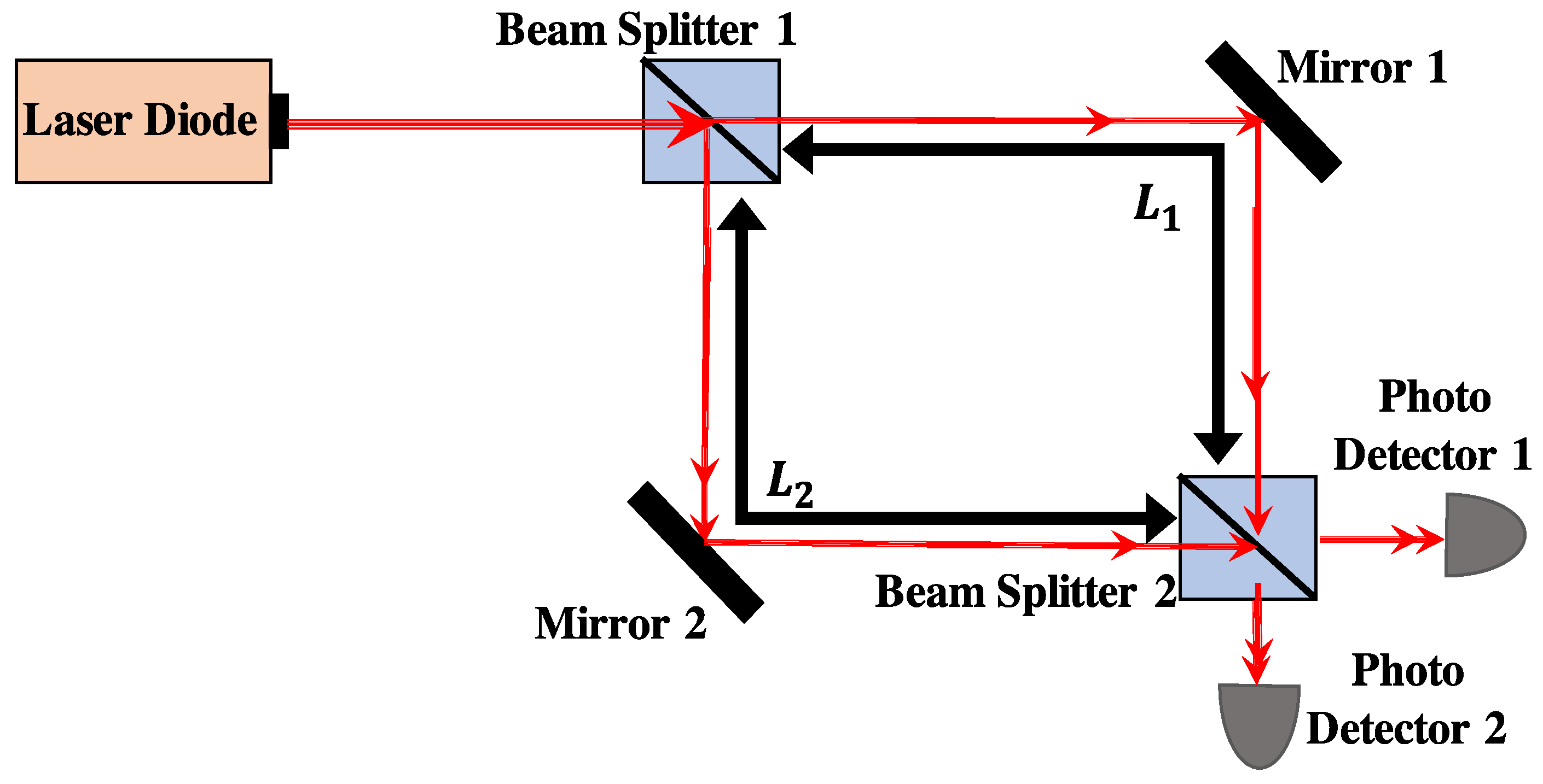
Figure 2.
Optical homodyne detection.

Figure 3.
Self-mixing homodyne detection for heartbeat measurement.
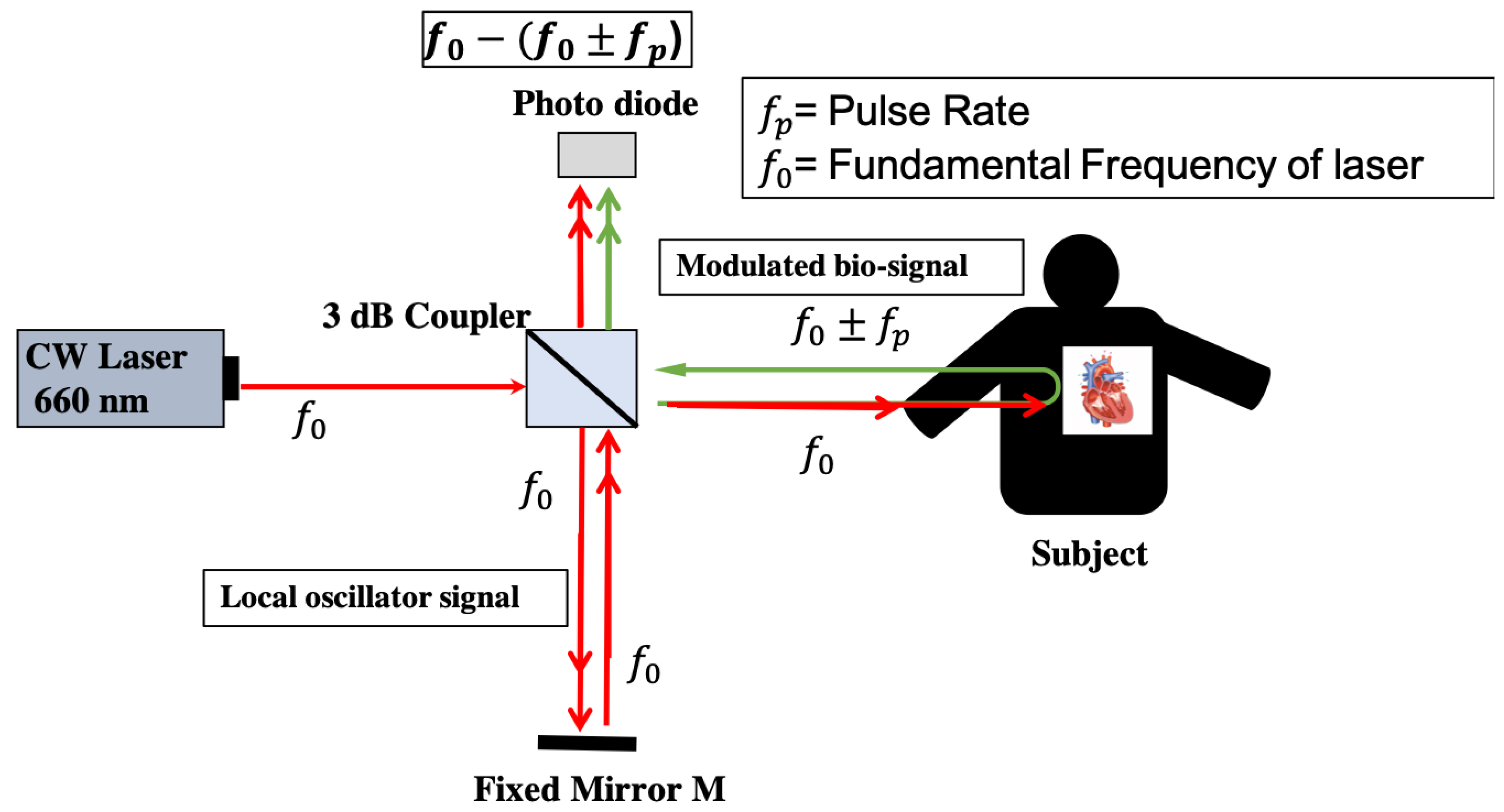
Figure 4.
Structure of AOM.
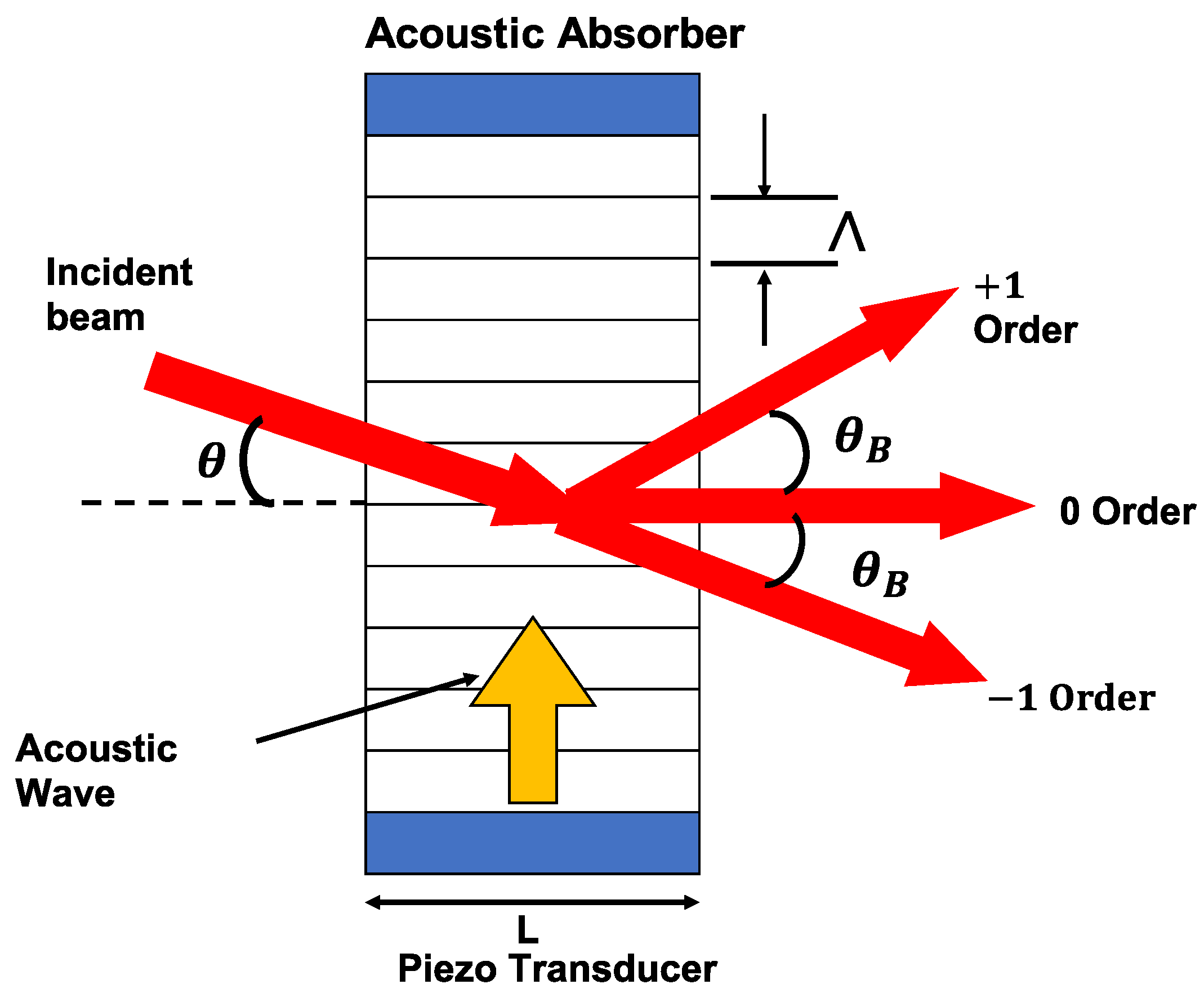
Figure 5.
Optical heterodyne detection.

Figure 6.
Self-mixing heterodyne detection with M–Z interferometer.

Figure 7.
Self-mixing heterodyne detection with human test subject.
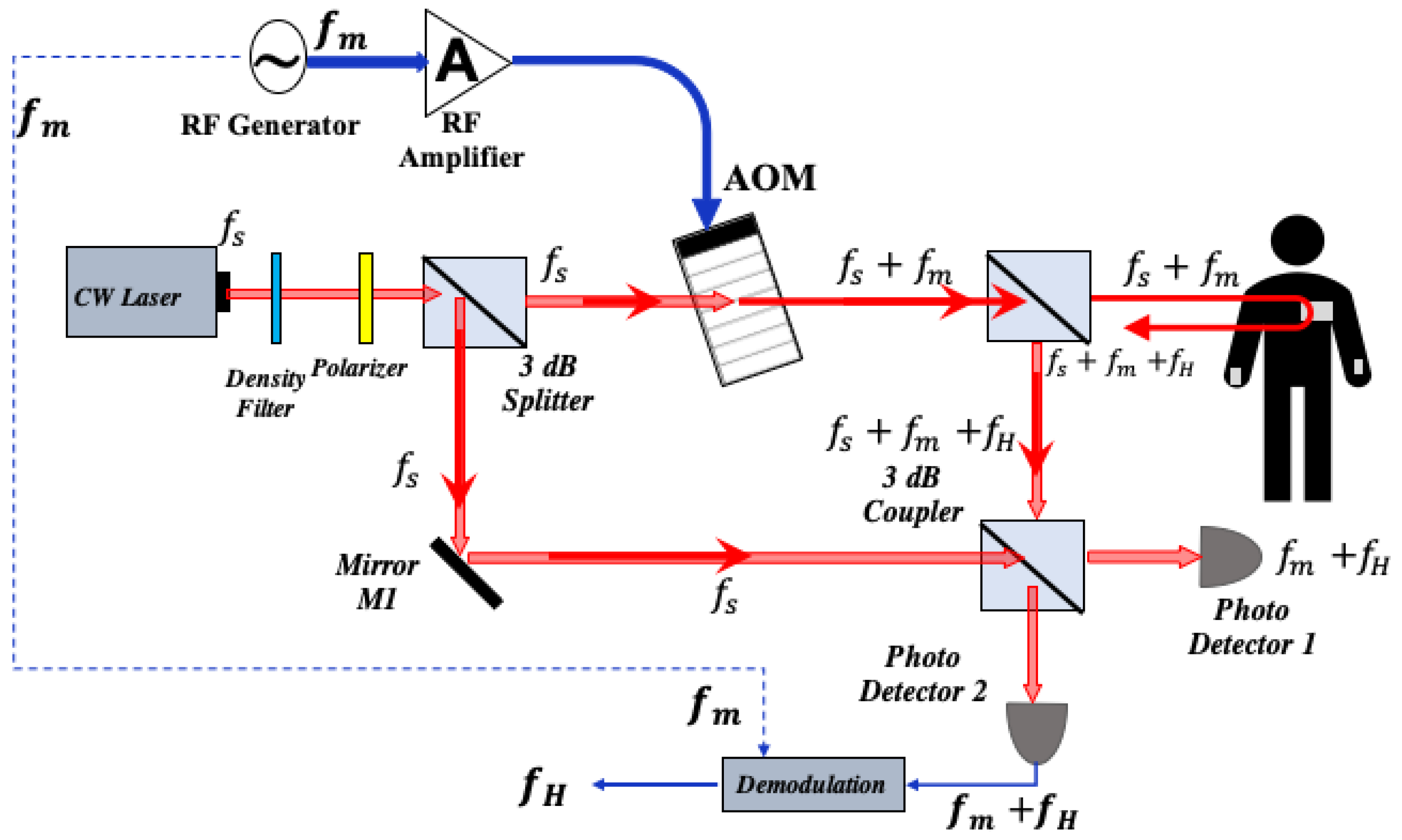
Figure 8.
(a) Gold deposition process on silica substrate; (b) thin film reflector on wrist position.
Figure 8.
(a) Gold deposition process on silica substrate; (b) thin film reflector on wrist position.

Figure 9.
HR detection with optical homodyne technique.
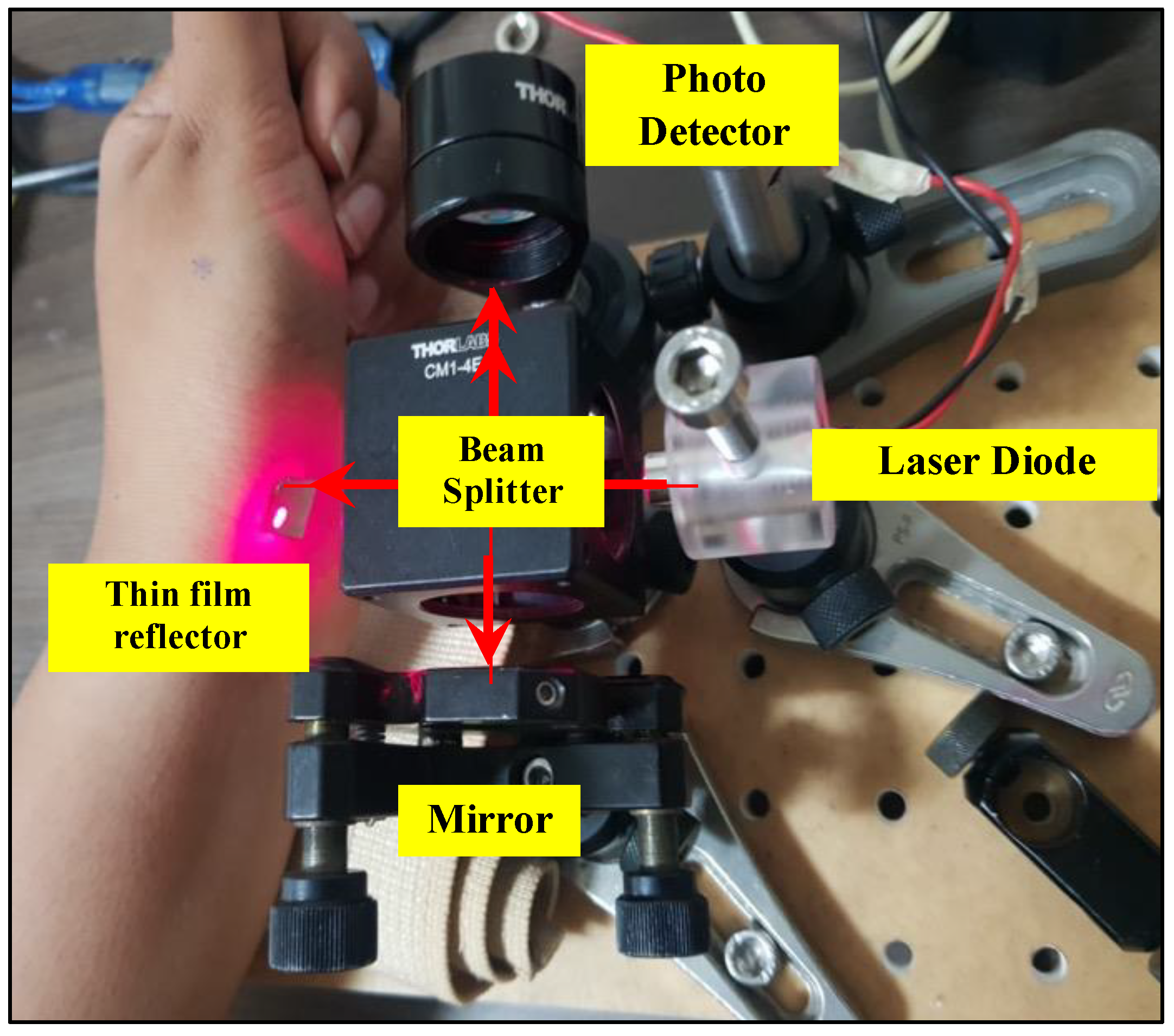
Figure 10.
HR detection on wrist position with optical homodyne technique.
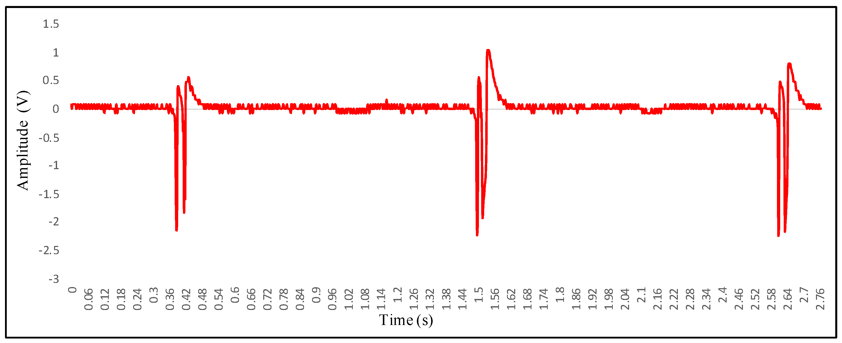
Figure 11.
(a) Working of AOM; (b) observation of higher order modes after modulation of laser from AOM.
Figure 11.
(a) Working of AOM; (b) observation of higher order modes after modulation of laser from AOM.
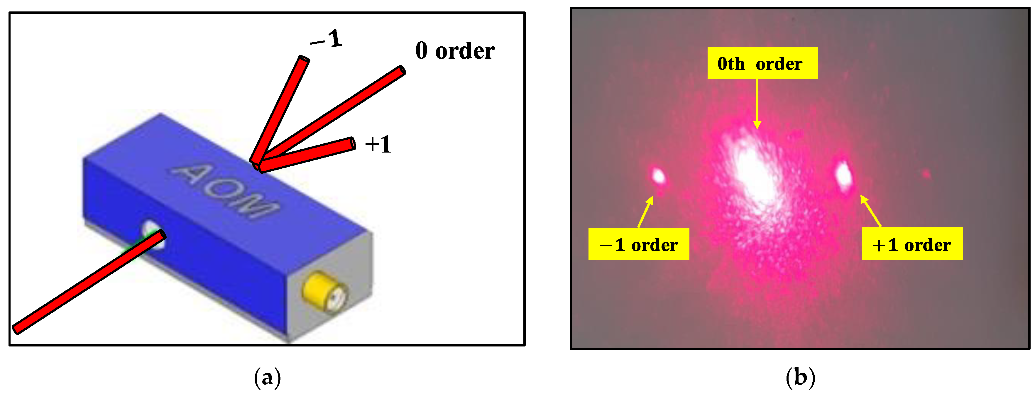
Figure 12.
First order modulation of 660 nm laser with AOM with central frequency 60 MHz.

Figure 13.
(a) Experimental setup for optical heterodyne detection; (b) measurement on human wrist position.
Figure 13.
(a) Experimental setup for optical heterodyne detection; (b) measurement on human wrist position.
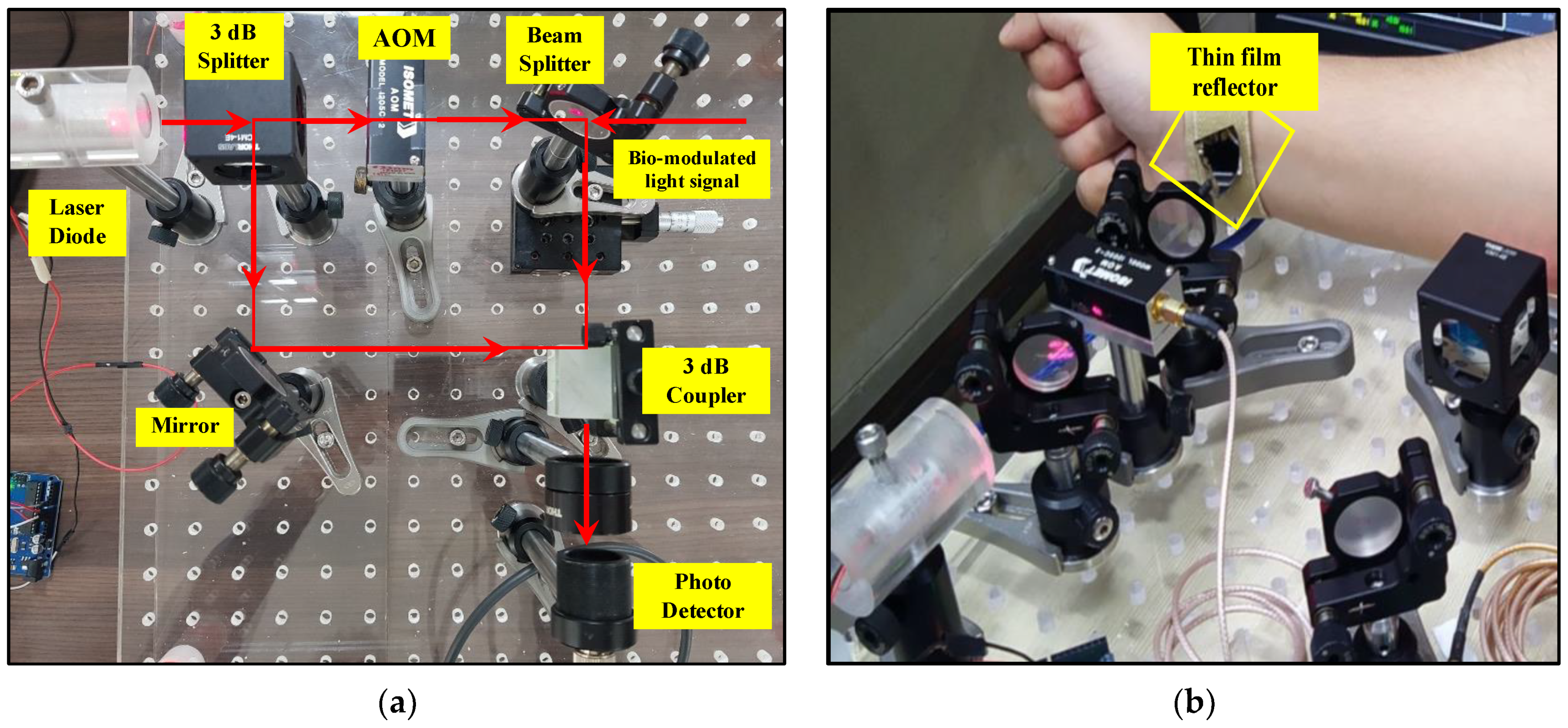
Figure 14.
Modulation frequency along with chest wall frequency detection.
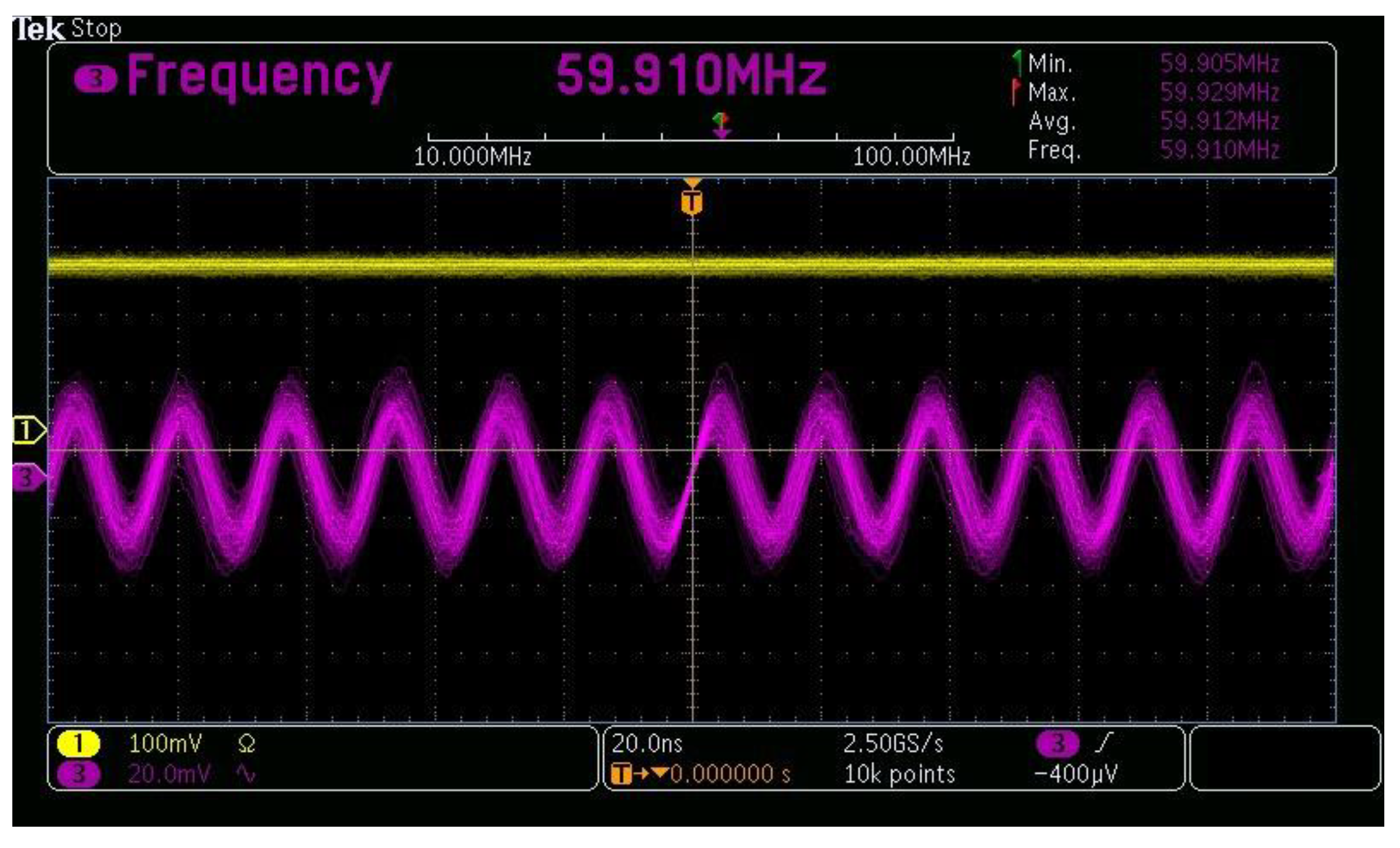
Figure 15.
Modulation frequency along with chest wall frequency detection.
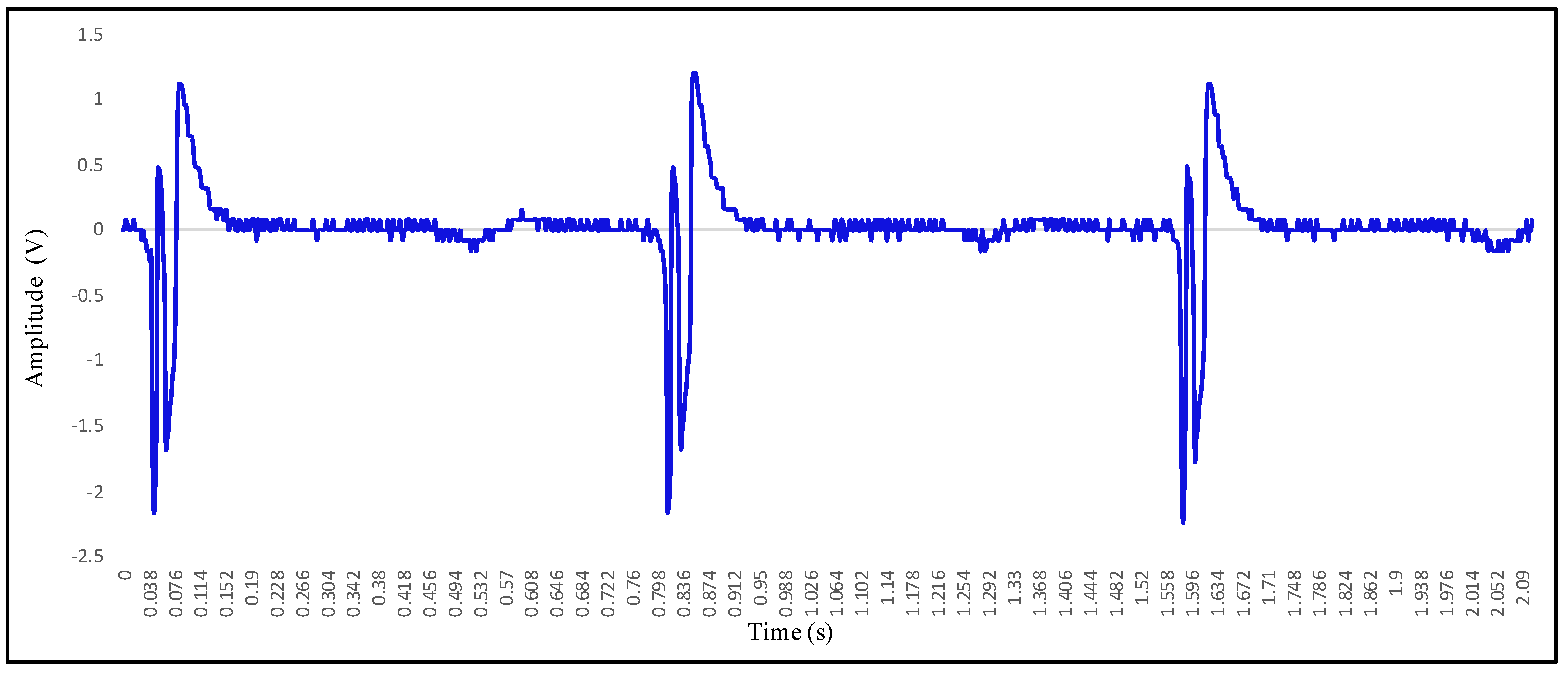
Figure 16.
ECG and VCG signal for 72 heart beats per minute.
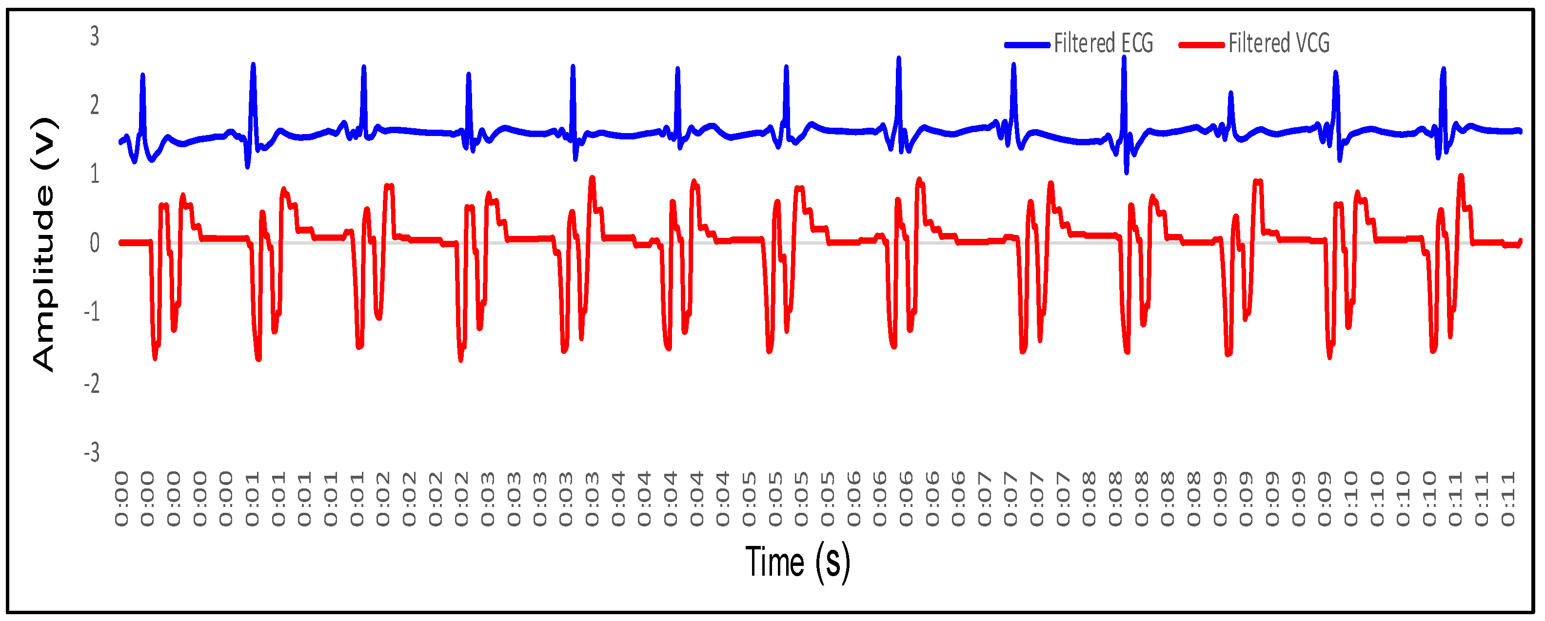
Figure 17.
ECG and VCG signal for 78 heart beats per minute.
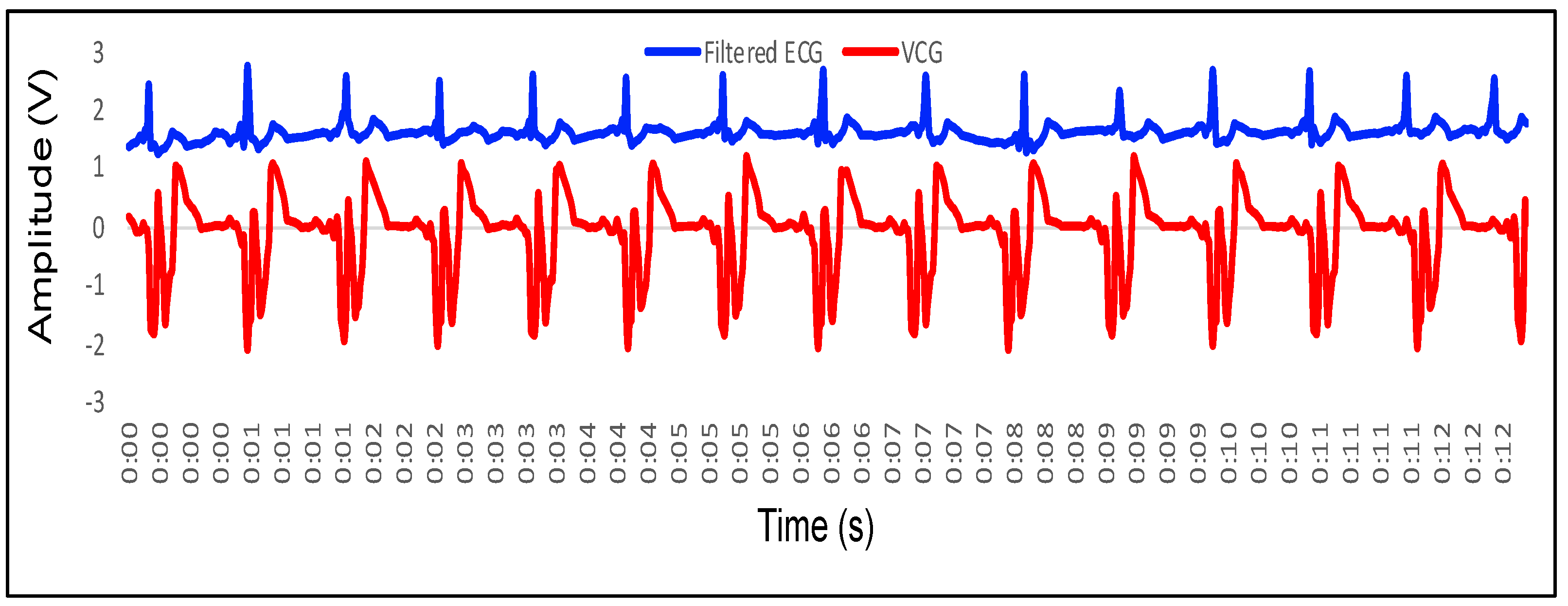
Figure 18.
ECG and VCG signal for 84 heart beats per minute.
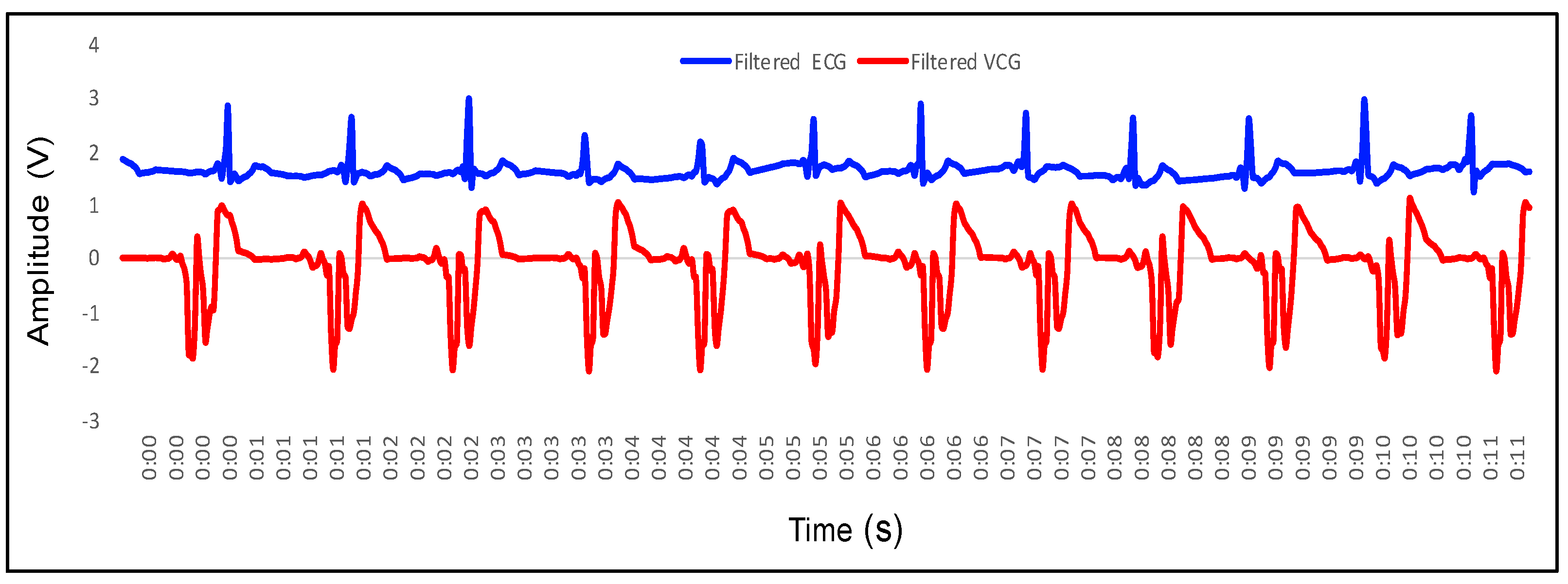
Figure 19.
ECG and VCG signal for 90 heart beats per minute.
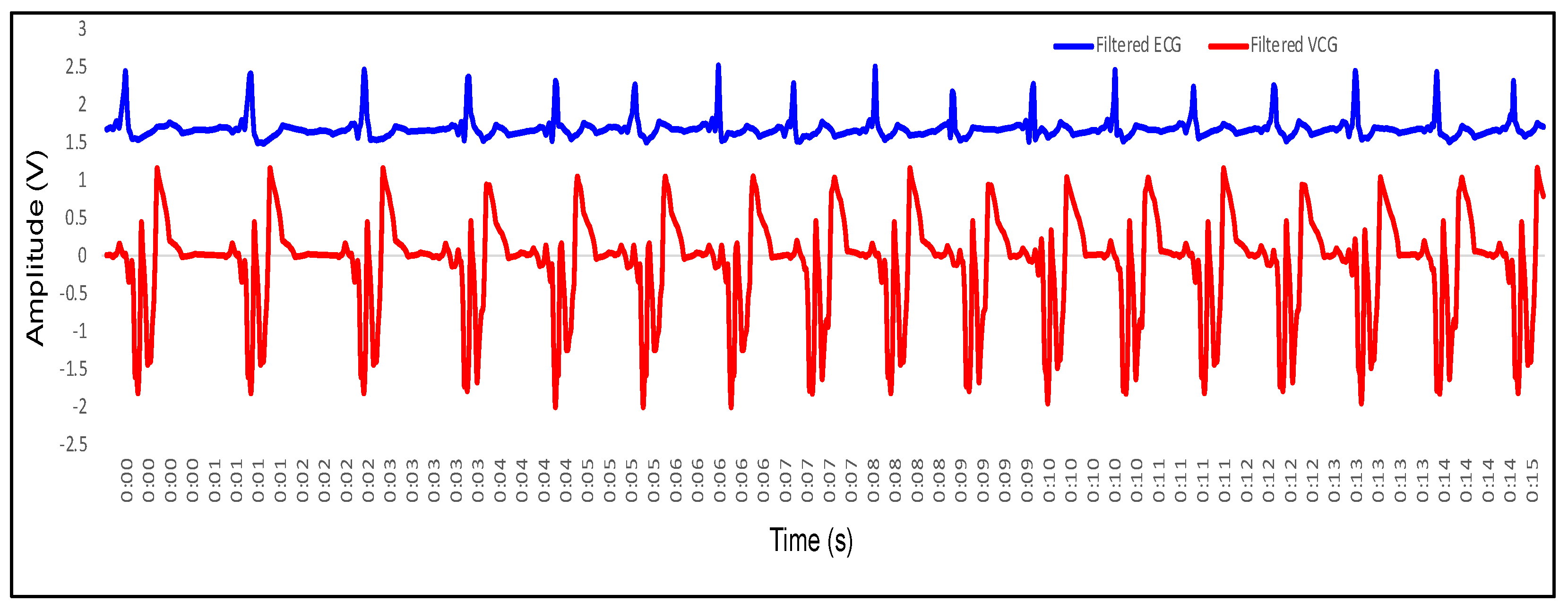
Figure 20.
ECG and VCG signal for 96 heart beats per minute.
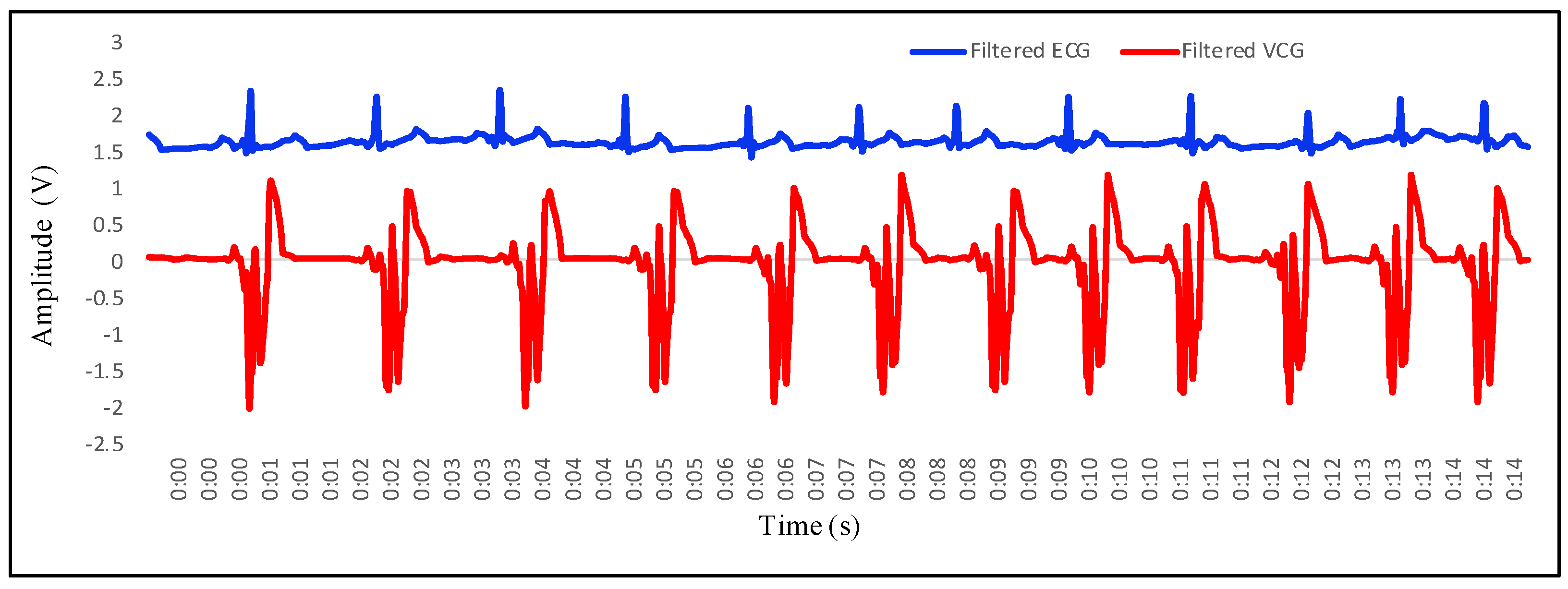
Figure 21.
ECG and VCG signal for 102 heart beats per minute.

Figure 22.
ECG and VCG signal for 108 heart beats per minute.
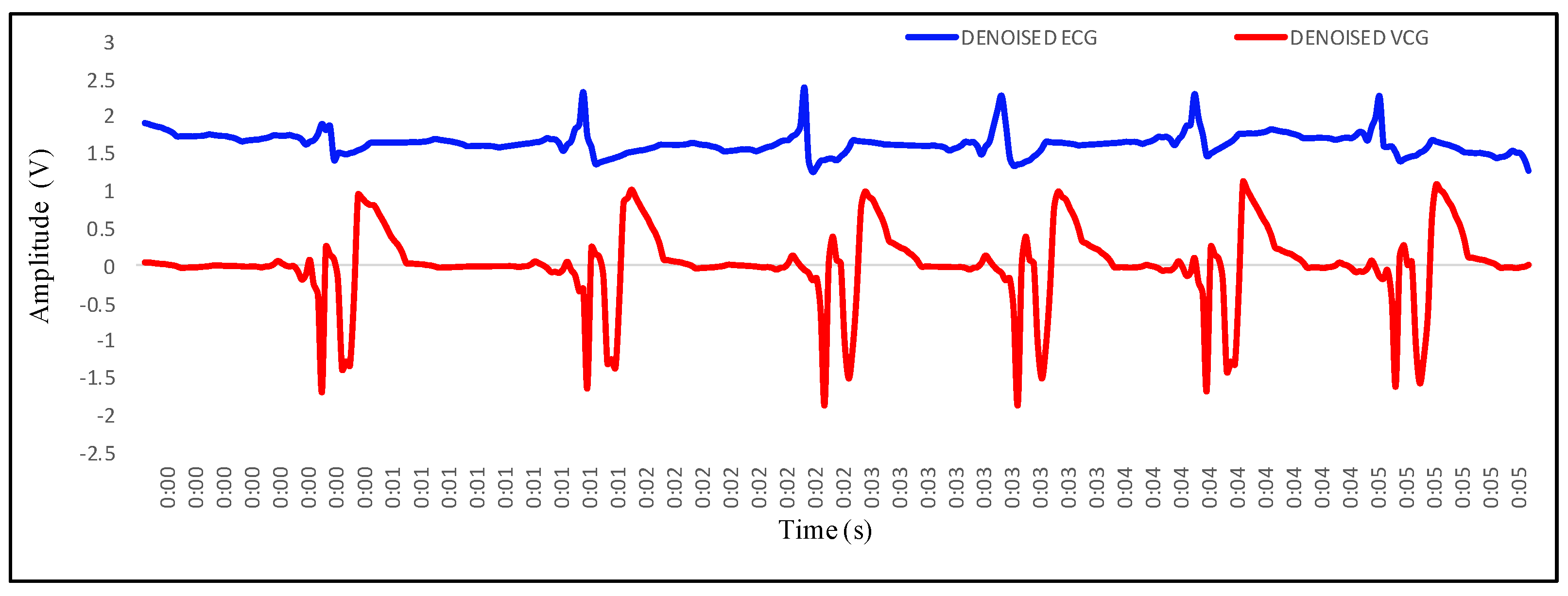
Figure 23.
VCG signals obtained for different values of HR: VCG1, 72 bpm; VCG2, 90 bpm; VCG3, 102 bpm.
Figure 23.
VCG signals obtained for different values of HR: VCG1, 72 bpm; VCG2, 90 bpm; VCG3, 102 bpm.

Figure 24.
Mapping of P wave of ECG and wave of VCG.
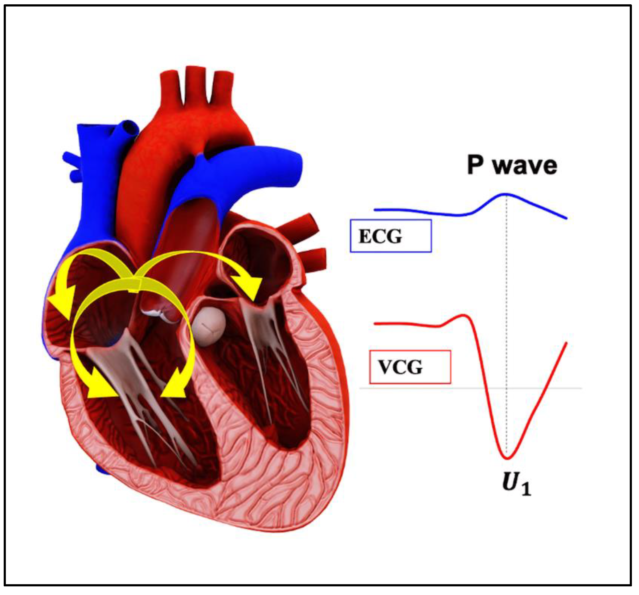
Figure 25.
Mapping of QRS complex of ECG and complex of VCG.

Figure 26.
Mapping of T wave of ECG and wave of VCG.

Figure 27.
Mapping of complete ECG wave with VCG wave.
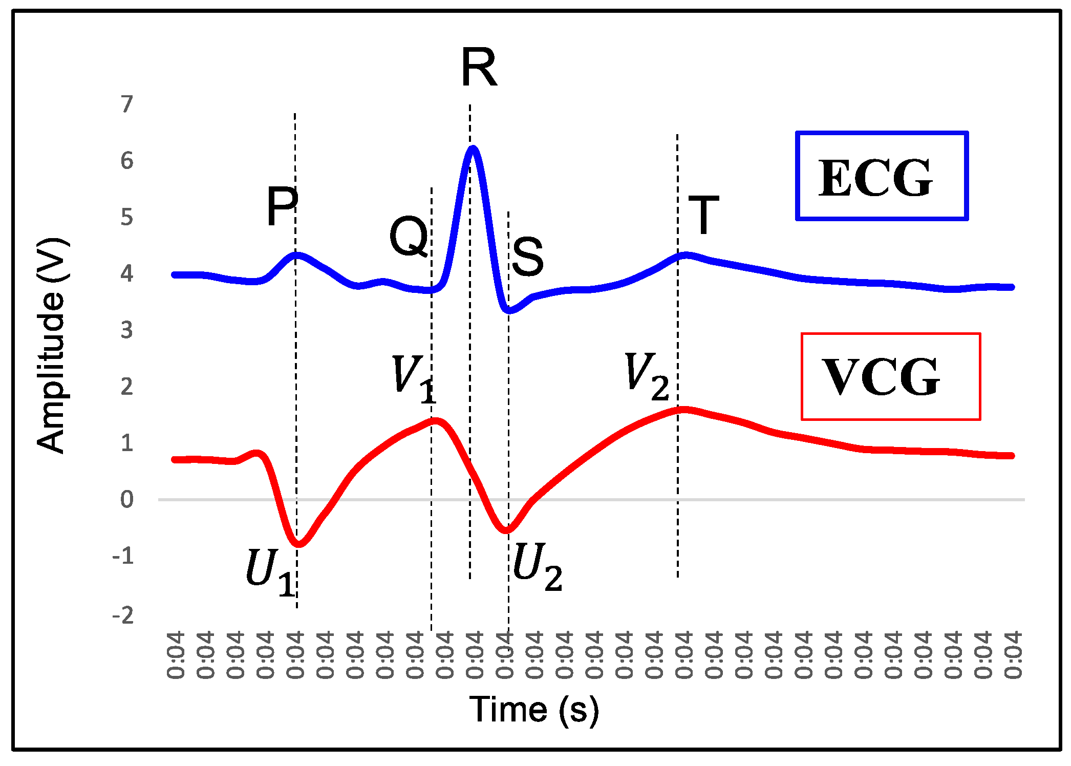
Figure 28.
Comparison of R-R, U-U, and V-V variability from ECG and VCG for HR 60 bpm.

Figure 29.
Comparison of R-R and V-V variability from ECG and VCG for test subject under sleep.

Figure 30.
Comparison of R-R and V-V variability from ECG and VCG for HR 54 bpm.

Figure 31.
Comparison of R-R and V-V variability from ECG and VCG for HR 72 bpm.
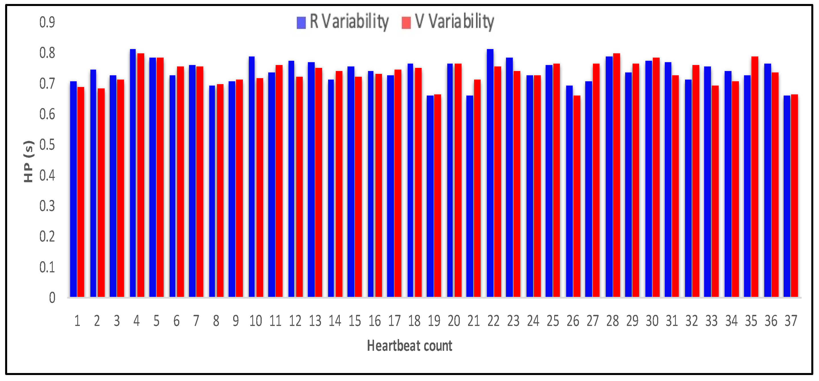
Figure 32.
Comparison of R-R and V-V variability from ECG and VCG for HR 96 bpm.
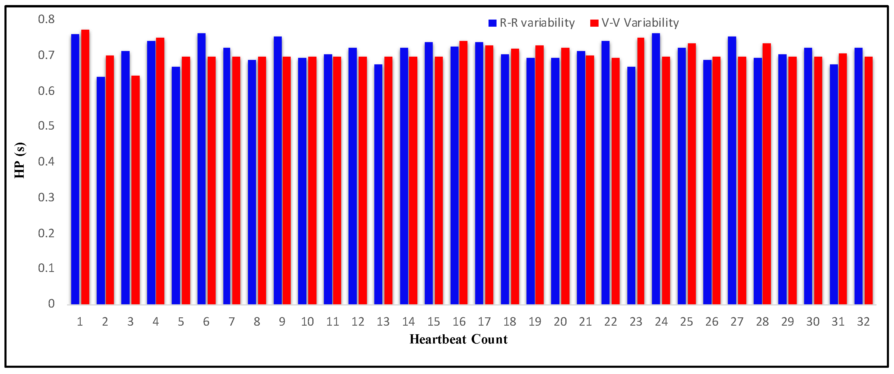
Figure 33.
Comparison of R-R and V-V variability from ECG and VCG for HR 108 bpm.
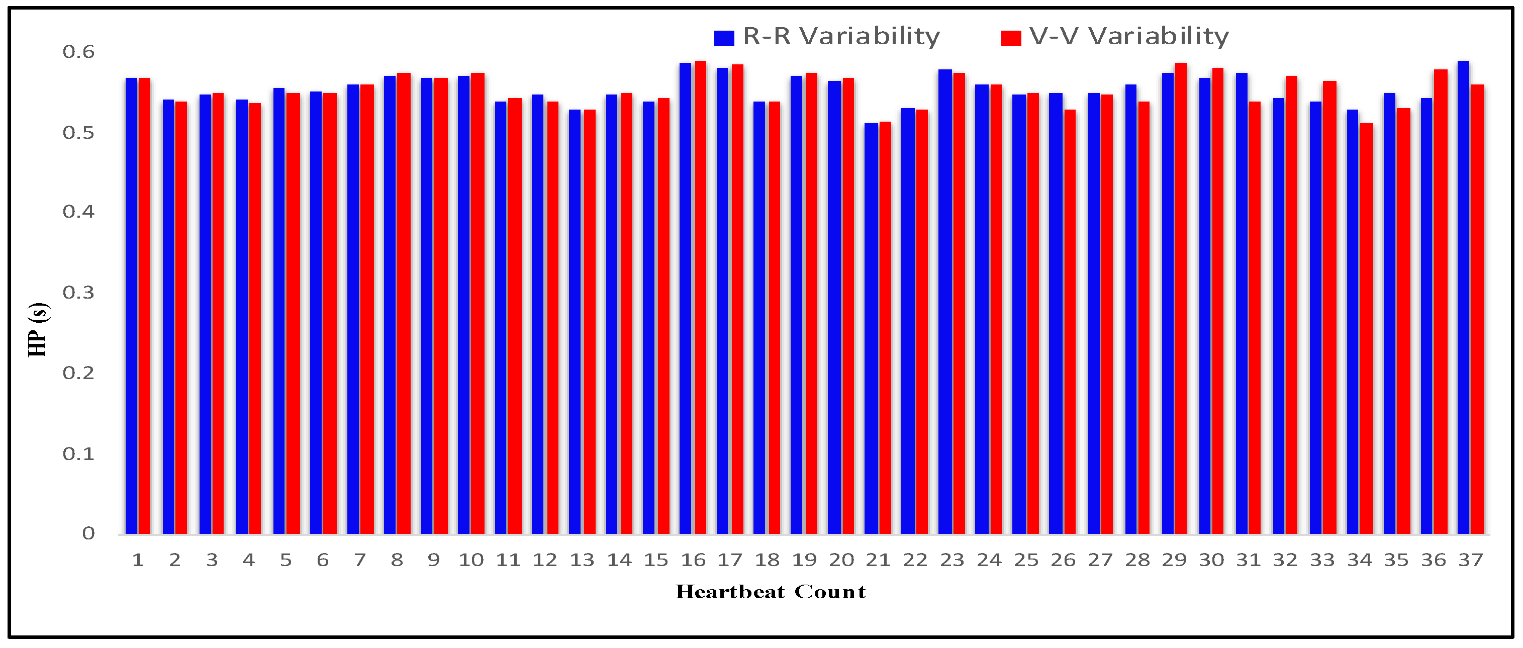
Figure 34.
R-R and V-V variability from ECG and VCG for different values of HR.

Figure 35.
(a) Mapping of homodyne and heterodyne VCG trace for measurement of HR 54 bpm; (b) mapping of homodyne and heterodyne VCG trace for measurement of HR 84 bpm.
Figure 35.
(a) Mapping of homodyne and heterodyne VCG trace for measurement of HR 54 bpm; (b) mapping of homodyne and heterodyne VCG trace for measurement of HR 84 bpm.

Figure 36.
(a) Mapping of optical heterodyne VCG trace with ECG for measurement of HR more than 70 bpm; (b) mapping of optical homodyne VCG trace with ECG for measurement of HR more than 70 bpm.
Figure 36.
(a) Mapping of optical heterodyne VCG trace with ECG for measurement of HR more than 70 bpm; (b) mapping of optical homodyne VCG trace with ECG for measurement of HR more than 70 bpm.
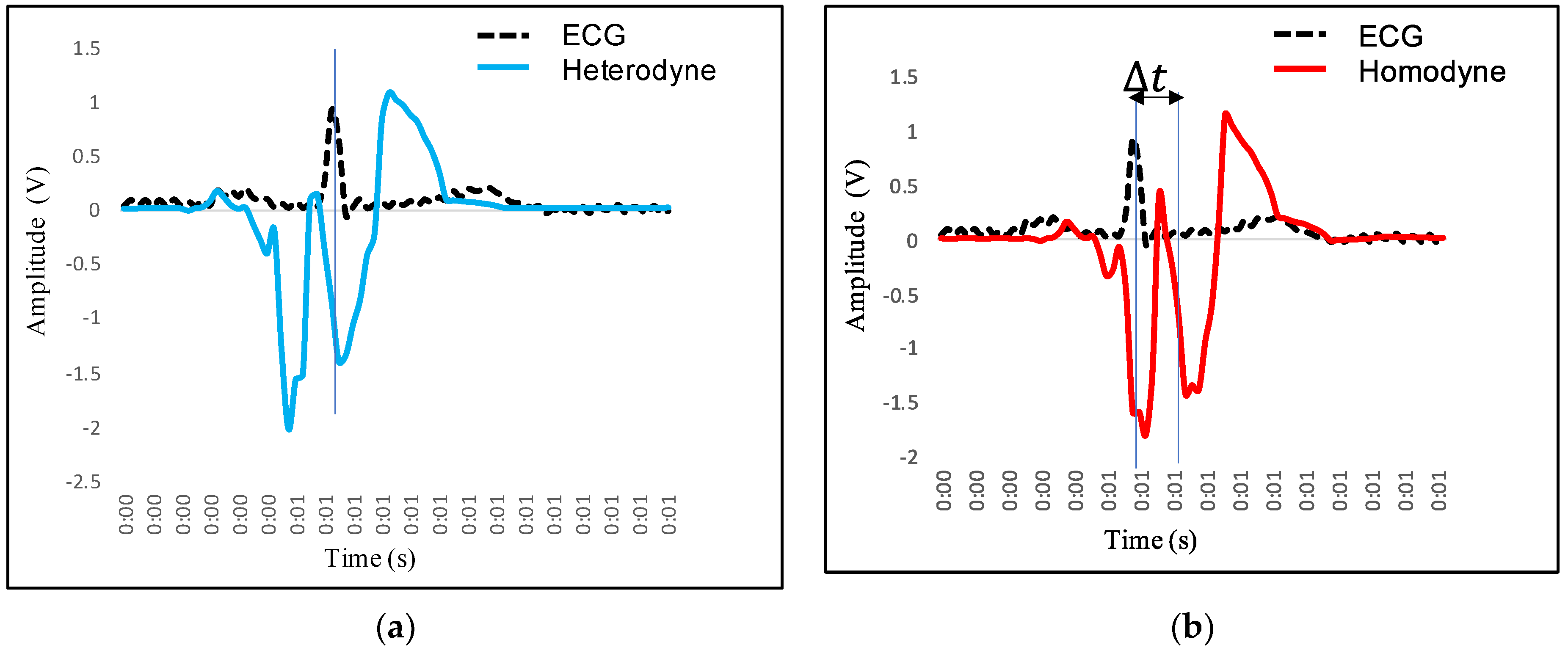
Figure 37.
Deviation of heterodyne and homodyne measurement from ECG.
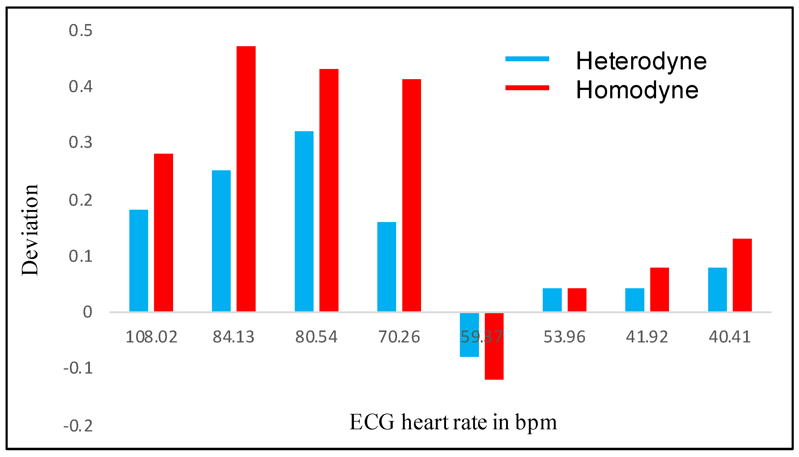
Figure 38.
(a) Deviations of HR measured with heterodyne system with respect to ECG (chest wall measurement, subject 7); (b) deviations of HR measured with homodyne system with respect to ECG (chest wall measurement, subject 7).
Figure 38.
(a) Deviations of HR measured with heterodyne system with respect to ECG (chest wall measurement, subject 7); (b) deviations of HR measured with homodyne system with respect to ECG (chest wall measurement, subject 7).

Table 1.
AOM specification.
| Parameter | Specification |
|---|---|
| Material | Lead molybdate |
| Active aperture | 2 mm |
| Center frequency | 60 MHz |
| Center wavelength | 660 nm |
Table 2.
Specification of RF generator and amplifier.
| Parameter | Specification |
|---|---|
| RF signal generator voltage | 12 V |
| RF signal generator output frequency | 70 MHz–200 MHz |
| Output power RF generator | 10 dBm |
| RF amplifier supply voltage | 12 V DC |
| RF amplifier gain | 32 dB |
Table 3.
Characteristics of test subjects under test.
| Subject Number | Gender | Age (Years) | Weight (kg) | Height (m) | Body Mass Index (BMI) (kg·m−2) |
|---|---|---|---|---|---|
| 1 | M | 20 | 61 | 1.71 | 20.86 |
| 2 | M | 20 | 59 | 1.69 | 20.65 |
| 3 | M | 22 | 64 | 1.73 | 21.38 |
| 4 | M | 22 | 66 | 1.75 | 21.55 |
| 5 | M | 25 | 68 | 1.79 | 21.22 |
| 6 | M | 25 | 64 | 1.75 | 20.89 |
| 7 | M | 30 | 65 | 1.70 | 22.49 |
| 8 | M | 32 | 67 | 1.84 | 19.78 |
| 9 | M | 38 | 69 | 1.77 | 22.02 |
| 10 | M | 40 | 70 | 1.76 | 22.59 |
| 11 | F | 20 | 55 | 1.76 | 17.75 |
| 12 | F | 20 | 53 | 1.71 | 18.12 |
| 13 | F | 22 | 57 | 1.74 | 18.82 |
| 14 | F | 25 | 64 | 1.78 | 20.20 |
| 15 | F | 25 | 58 | 1.73 | 19.37 |
| 16 | F | 28 | 68 | 1.80 | 20.98 |
| 17 | F | 30 | 64 | 1.78 | 20.19 |
| 18 | F | 32 | 63 | 1.70 | 21.79 |
| 19 | F | 38 | 67 | 1.75 | 21.87 |
| 20 | F | 40 | 69 | 1.65 | 25.34 |
Table 4.
Heart period and HRV measurement for test subject under relax condition with ECG and VCG analysis.
Table 4.
Heart period and HRV measurement for test subject under relax condition with ECG and VCG analysis.
| Heartbeat Count | R Period (s) | R-R Variability (s) | U Period (s) | V Period (s) | V-V Variability (s) |
|---|---|---|---|---|---|
| 1 | 0.256836 | - | 0.23564 | 0.27564 | - |
| 2 | 1.283203 | 1.026367 | 1.207031 | 1.247031 | 0.971391 |
| 3 | 2.301758 | 1.018555 | 2.2177735 | 2.2577735 | 1.0107425 |
| 4 | 3.321289 | 1.019531 | 3.2285155 | 3.2685155 | 1.010742 |
| 5 | 4.28125 | 0.959961 | 4.25 | 4.29 | 1.0214845 |
| 6 | 5.303711 | 1.022461 | 5.2714845 | 5.3114845 | 1.0214845 |
| 7 | 6.291992 | 0.988281 | 6.2929685 | 6.3329685 | 1.021484 |
| 8 | 7.303711 | 1.011719 | 7.314453 | 7.354453 | 1.0214845 |
| 9 | 8.256836 | 0.953125 | 8.324453 | 8.364453 | 1.01 |
| 10 | 9.303711 | 1.046875 | 9.364453 | 9.404453 | 1.04 |
| 11 | 10.2978515 | 0.9941405 | 10.324453 | 10.364453 | 0.96 |
| 12 | 11.3427735 | 1.044922 | 11.2914453 | 11.3314453 | 0.9669923 |
| 13 | 12.2714845 | 0.928711 | 12.3214453 | 12.3614453 | 1.03 |
| 14 | 13.276367 | 1.0048825 | 13.314453 | 13.354453 | 0.9930077 |
| 15 | 14.256836 | 0.980469 | 14.314453 | 14.354453 | 1 |
| 16 | 15.321289 | 1.064453 | 15.3231445 | 15.3631445 | 1.00869153 |
| 17 | 16.41289 | 1.091601 | 16.354453 | 16.394453 | 1.03130847 |
| 18 | 17.361289 | 0.948399 | 17.384453 | 17.424453 | 1.03 |
| 19 | 18.381289 | 1.02 | 18.384453 | 18.424453 | 1 |
| 20 | 19.5289 | 1.147611 | 19.434453 | 19.474453 | 1.05 |
Table 5.
Analysis of variability from RR and VV interval (measurement on chest wall).
| Subject No. | R-R Variability ECG (ms) | V-V Variability Heterodyne (ms) | V-V Variability Homodyne (ms) | HR in bpm (ECG) | HR in bpm (Heterodyne) | HR in bpm (Homodyne) |
|---|---|---|---|---|---|---|
| 1 | 555 ± 3 | 554.5 ± 3 | 554 ± 3 | 108.02 | 108.20 | 108.30 |
| 15 | 713 ± 5 | 711 ± 3 | 709 ± 5 | 84.13 | 84.38 | 84.60 |
| 12 | 745 ± 6 | 742 ± 3 | 741 ± 6 | 80.54 | 80.86 | 80.97 |
| 16 | 854 ± 8 | 852 ± 4 | 849 ± 5 | 70.26 | 70.42 | 70.67 |
| 5 | 1010 ± 6 | 1012 ± 4 | 1012 ± 4 | 59.37 | 59.29 | 59.25 |
| 7 | 1112 ± 6 | 1111 ± 6 | 1111 ± 6 | 53.96 | 54.00 | 54.00 |
| 19 | 1431 ± 10 | 1430 ± 8 | 1429 ± 8 | 41.92 | 41.96 | 42.00 |
| 10 | 1484 ± 17 | 1482 ± 8 | 1480 ± 15 | 40.41 | 40.54 | 40.68 |
Table 6.
Deviation in HR for optical homodyne and heterodyne detection.
| Subject Number | HR in bpm (ECG) | HR in bpm (Heterodyne) | HR in bpm (Homodyne) | Deviation in bpm (Heterodyne) | Deviation in bpm (Homodyne) |
|---|---|---|---|---|---|
| 1 | 108.02 | 108.2 | 108.3 | 0.18 | 0.28 |
| 15 | 84.13 | 84.38 | 84.6 | 0.25 | 0.47 |
| 12 | 80.54 | 80.86 | 80.97 | 0.32 | 0.43 |
| 16 | 70.26 | 70.42 | 70.67 | 0.16 | 0.41 |
| 5 | 59.37 | 59.29 | 59.25 | −0.08 | −0.12 |
| 7 | 53.96 | 54 | 54 | 0.04 | 0.04 |
| 19 | 41.92 | 41.96 | 42 | 0.04 | 0.08 |
| 10 | 40.41 | 40.49 | 40.54 | 0.08 | 0.13 |
Table 7.
Deviation in HR for optical homodyne and heterodyne detection.
| Subject No. | Measurement Site | HR in bpm (Homodyne) | HR in bpm (Heterodyne) |
|---|---|---|---|
| 5 | Coronary Artery | 59.29 | 59.25 |
| 5 | Radial Artery | 60.12 | 60.04 |
| 15 | Coronary Artery | 84.38 | 84.6 |
| 15 | Radial Artery | 85.22 | 84.9 |
Publisher’s Note: MDPI stays neutral with regard to jurisdictional claims in published maps and institutional affiliations. |
© 2021 by the authors. Licensee MDPI, Basel, Switzerland. This article is an open access article distributed under the terms and conditions of the Creative Commons Attribution (CC BY) license (https://creativecommons.org/licenses/by/4.0/).
Share and Cite
MDPI and ACS Style
Gondane, J.; Panse, M.S. Development of an Optical System for Non-Contact Type Measurement of Heart Rate and Heart Rate Variability. Appl. Syst. Innov. 2021, 4, 48. https://doi.org/10.3390/asi4030048
AMA Style
Gondane J, Panse MS. Development of an Optical System for Non-Contact Type Measurement of Heart Rate and Heart Rate Variability. Applied System Innovation. 2021; 4(3):48. https://doi.org/10.3390/asi4030048
Chicago/Turabian StyleGondane, Jyoti, and Meena S. Panse. 2021. "Development of an Optical System for Non-Contact Type Measurement of Heart Rate and Heart Rate Variability" Applied System Innovation 4, no. 3: 48. https://doi.org/10.3390/asi4030048