
Smartphone LiDAR Technologies for Surveying and Reality Modelling in Urban Scenarios: Evaluation Methods, Performance and Challenges


Abstract
:1. Introduction
1.1. Literature Review
1.2. Aim and Organization of the Paper
2. Materials and Methods
2.1. Mobile Devices and Scanning Apps
2.2. Research Methodology
2.2.1. Phase 1: 3D Survey by Smartphone Depth Sensors
2.2.2. Phase 2: Point Clouds Analysis
3. Results
3.1. Laboratory Testing under Controlled Conditions
3.2. Field Tests and Applications under Real Conditions
4. Discussion
5. Conclusions
Author Contributions
Funding
Institutional Review Board Statement
Informed Consent Statement
Data Availability Statement
Conflicts of Interest
Appendix A

| Sample Material | Scan Distance: 0.5 m | Scan Distance: 1.5 m | ||||
|---|---|---|---|---|---|---|
| SVλ 1 cm | SVλ 1.5 cm | SVλ 2 cm | SVλ 1 cm | SVλ 1.5 cm | SVλ 2 cm | |
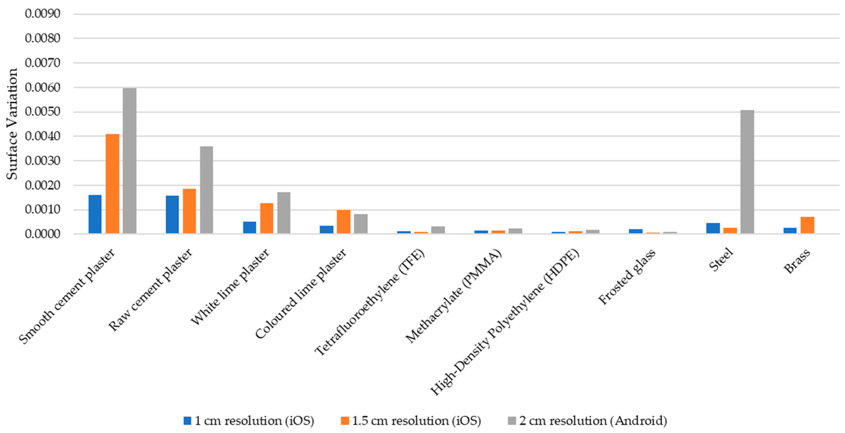
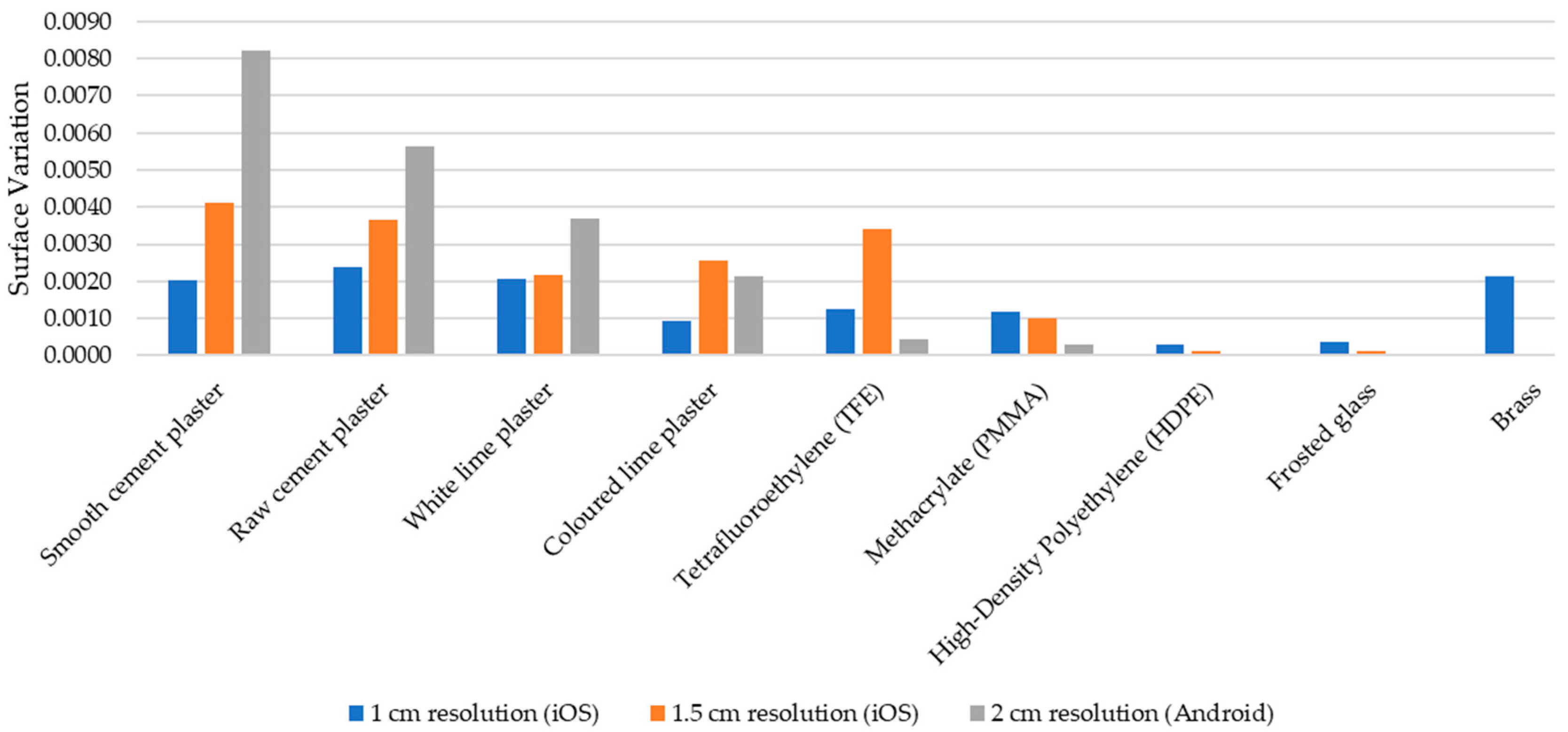
| Smooth cement plaster | 0.0020 | 0.0041 | 0.0082 | 0.0016 | 0.0041 | 0.0060 |
| Raw cement plaster | 0.0024 | 0.0037 | 0.0056 | 0.0016 | 0.0019 | 0.0036 |
| White lime plaster | 0.0021 | 0.0022 | 0.0037 | 0.0005 | 0.0013 | 0.0017 |
| Coloured lime plaster | 0.0009 | 0.0026 | 0.0021 | 0.0004 | 0.0010 | 0.0008 |
| Tetrafluoroethylene (TFE) | 0.0013 | 0.0034 | 0.0004 | 0.0001 | 0.0001 | 0.0003 |
| Methacrylate (PMMA) | 0.0012 | 0.0010 | 0.0003 | 0.0002 | 0.0002 | 0.0003 |
| High-density polyethylene (HDPE) | 0.0003 | 0.0001 | 0.0001 | 0.0001 | 0.0001 | 0.0002 |
| Frosted glass | 0.0004 | 0.0001 | 0.0001 | 0.0002 | 0.0001 | 0.0001 |
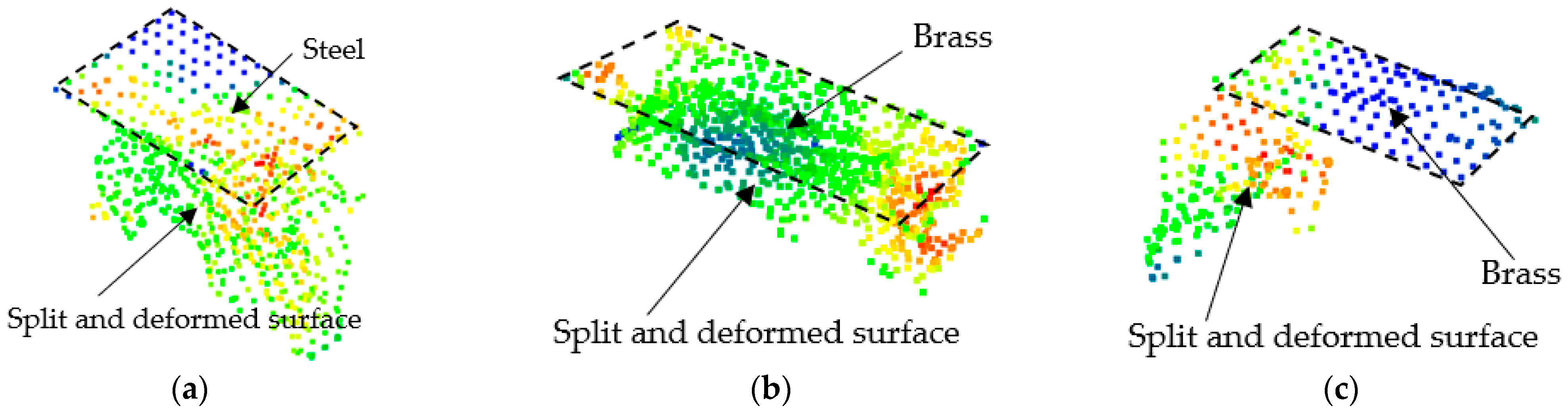
| Steel | No data | No data | 0.1672 | 0.0005 | 0.0003 | 0.0051 |
| Brass | 0.0021 | 0.1455 | 0.1000 | 0.0003 | 0.0007 | 0.0142 |

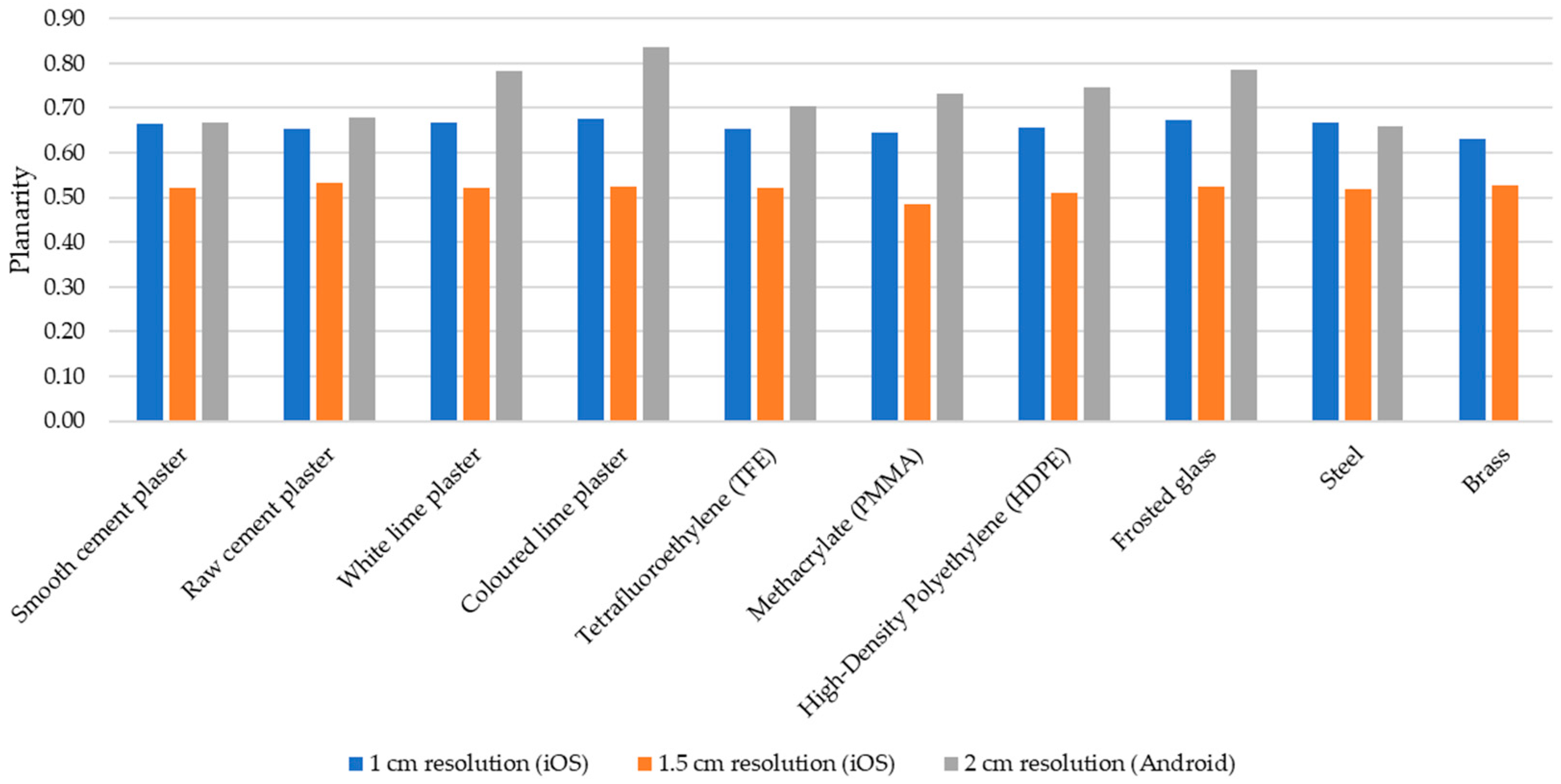
| Sample Material | Scan Distance: 0.5 m | Scan Distance: 1.5 m | ||||
|---|---|---|---|---|---|---|
| Pλ 1 cm | Pλ 1.5 cm | Pλ 2 cm | Pλ 1 cm | Pλ 1.5 cm | Pλ 2 cm | |
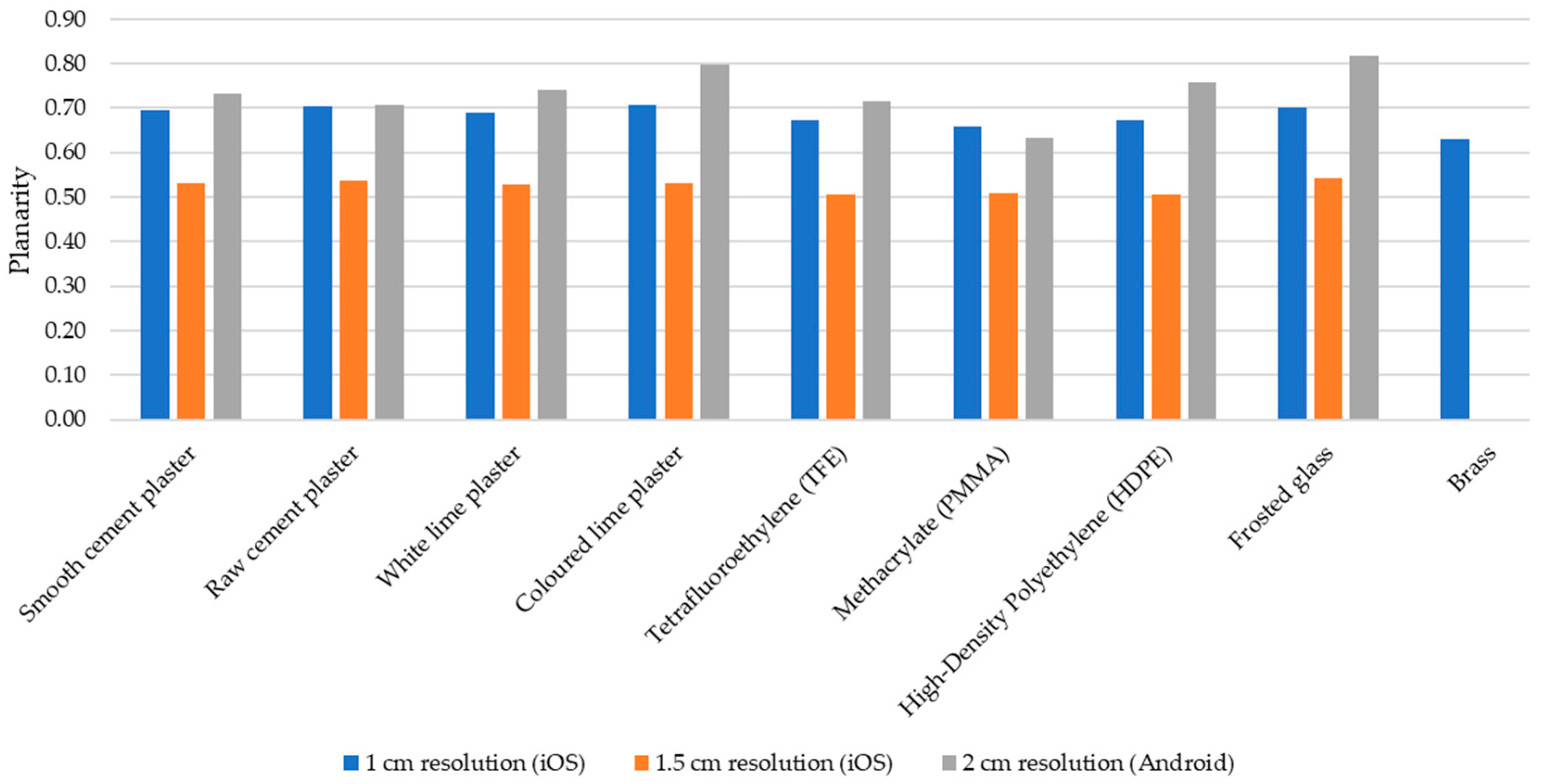
| Smooth cement plaster | 0.70 | 0.53 | 0.73 | 0.66 | 0.52 | 0.67 |
| Raw cement plaster | 0.70 | 0.54 | 0.71 | 0.65 | 0.53 | 0.68 |
| White lime plaster | 0.69 | 0.53 | 0.74 | 0.67 | 0.52 | 0.78 |
| Coloured lime plaster | 0.71 | 0.53 | 0.80 | 0.67 | 0.52 | 0.84 |
| Tetrafluoroethylene (TFE) | 0.67 | 0.50 | 0.72 | 0.65 | 0.52 | 0.70 |
| Methacrylate (PMMA) | 0.66 | 0.51 | 0.63 | 0.65 | 0.48 | 0.73 |
| High-density polyethylene (HDPE) | 0.67 | 0.51 | 0.76 | 0.66 | 0.51 | 0.75 |
| Frosted glass | 0.70 | 0.54 | 0.82 | 0.67 | 0.52 | 0.79 |
| Steel | No data | No data | - | 0.67 | 0.52 | 0.66 |
| Brass | 0.63 | - | - | 0.63 | 0.53 | - |

Appendix B


References
- Mikita, T.; Balková, M.; Bajer, A.; Cibulka, M.; Patočka, Z. Comparison of Different Remote Sensing Methods for 3D Modeling of Small Rock Outcrops. Sensors 2020, 20, 1663. [Google Scholar] [CrossRef] [PubMed] [Green Version]
- Luetzenburg, G.; Kroon, A.; Bjørk, A.A. Evaluation of the Apple IPhone 12 Pro LiDAR for an Application in Geosciences. Sci. Rep. 2021, 11, 22221. [Google Scholar] [CrossRef]
- Gollob, C.; Ritter, T.; Kraßnitzer, R.; Tockner, A.; Nothdurft, A. Measurement of Forest Inventory Parameters with Apple IPad Pro and Integrated LiDAR Technology. Remote Sens. 2021, 13, 3129. [Google Scholar] [CrossRef]
- Durrant-Whyte, H.; Bailey, T. Simultaneous Localization and Mapping: Part I. IEEE Robot. Autom. Mag. 2006, 13, 99–110. [Google Scholar] [CrossRef] [Green Version]
- Engelhard, N.; Endres, F.; Hess, J.; Sturm, J.; Burgard, W. Real-Time 3D Visual SLAM with a Hand-Held RGB-D Camera. In Proceedings of the RGB-D Workshop on 3D Perception in Robotics at the European Robotics Forum, Vasteras, Sweden, 8 April 2011; Volume 180, pp. 1–15. [Google Scholar]
- Diakité, A.A.; Zlatanova, S. FIRST EXPERIMENTS WITH THE TANGO TABLET FOR INDOOR SCANNING. ISPRS Ann. Photogramm. Remote Sens. Spat. Inf. Sci. 2016, 3, 67–72. [Google Scholar] [CrossRef] [Green Version]
- Tomaštík, J.; Saloň, Š.; Tunák, D.; Chudý, F.; Kardoš, M. Tango in Forests—An Initial Experience of the Use of the New Google Technology in Connection with Forest Inventory Tasks. Comput. Electron. Agric. 2017, 141, 109–117. [Google Scholar] [CrossRef]
- Hyyppä, J.; Virtanen, J.-P.; Jaakkola, A.; Yu, X.; Hyyppä, H.; Liang, X. Feasibility of Google Tango and Kinect for Crowdsourcing Forestry Information. Forests 2018, 9, 6. [Google Scholar] [CrossRef] [Green Version]
- Tsoukalos, D.; Drosos, V.; Tsolis, D.K. Attempting to Reconstruct a 3D Indoor Space Scene with a Mobile Device Using ARCore. In Proceedings of the 2021 12th International Conference on Information, Intelligence, Systems Applications (IISA), Chania Crete, Greece, 12–14 July 2021; pp. 1–6. [Google Scholar]
- Vogt, M.; Rips, A.; Emmelmann, C. Comparison of IPad Pro®’s LiDAR and TrueDepth Capabilities with an Industrial 3D Scanning Solution. Technologies 2021, 9, 25. [Google Scholar] [CrossRef]
- Spreafico, A.; Chiabrando, F.; Losè, L.T.; Tonolo, F.G. The Ipad Pro Built-In LIDAR Sensor: 3d Rapid Mapping Tests and Quality Assessment. Int. Arch. Photogramm. Remote Sens. Spat. Inf. Sci. 2021, 43, 63–69. [Google Scholar] [CrossRef]
- Riquelme, A.; Tomás, R.; Cano, M.; Pastor, J.L.; Jordá-Bordehore, L. Extraction of Discontinuity Sets of Rocky Slopes Using IPhone-12 Derived 3DPC and Comparison to TLS and SfM Datasets. IOP Conf. Ser. Earth Environ. Sci. 2021, 833, 012056. [Google Scholar] [CrossRef]
- Tavani, S.; Billi, A.; Corradetti, A.; Mercuri, M.; Bosman, A.; Cuffaro, M.; Seers, T.; Carminati, E. Smartphone Assisted Fieldwork: Towards the Digital Transition of Geoscience Fieldwork Using LiDAR-Equipped IPhones. Earth-Sci. Rev. 2022, 227, 103969. [Google Scholar] [CrossRef]
- Girardeau-Montaut, D. CloudCompare. France: EDF R&D Telecom ParisTech. 2016. Available online: http://pcp2019.ifp.uni-stuttgart.de/presentations/04-CloudCompare_PCP_2019_public.pdf (accessed on 5 May 2022).
- Costantino, D.; Pepe, M.; Angelini, M.G. Evaluation of reflectance for building materials classification with terrestrial laser scanner radiation. Acta Polytech. 2021, 61, 174–198. [Google Scholar] [CrossRef]
- Herban, S.; Costantino, D.; Alfio, V.S.; Pepe, M. Use of Low-Cost Spherical Cameras for the Digitisation of Cultural Heritage Structures into 3D Point Clouds. J. Imaging 2022, 8, 13. [Google Scholar] [CrossRef]
- Farella, E.M.; Torresani, A.; Remondino, F. Sparse point cloud filtering based on covariance features. Int. Arch. Photogramm. Remote Sens. Spat. Inf. Sci. 2019, XLII-2/W15, 465–472. [Google Scholar] [CrossRef] [Green Version]
- Pauly, M.; Gross, M.; Kobbelt, L.P. Efficient Simplification of Point-Sampled Surfaces. In Proceedings of the IEEE Visualization, (VIS 2002), Boston, MA, USA, 27 October–1 November 2002; pp. 163–170. [Google Scholar]
- Jolliffe, I. Principal Component Analysis: A Beginner’s Guide—I. Introduction and Application. Weather 1990, 45, 375–382. [Google Scholar] [CrossRef]
- Hackel, T.; Wegner, J.D.; Schindler, K. Contour Detection in Unstructured 3D Point Clouds. In Proceedings of the IEEE Computer Society Conference on Computer Vision and Pattern Recognition, Las Vegas, NV, USA, 27–30 June 2016; pp. 1610–1618. [Google Scholar]
- Moore, D.S.; Notz, W.I.; Fligner, M.A. The Basic Practice of Statistics; Macmillan Higher Education: New York, NY, USA, 2015; ISBN 1-4641-8678-2. [Google Scholar]
- Pepe, M.; Costantino, D.; Vozza, G.; Alfio, V.S. Comparison of Two Approaches to GNSS Positioning Using Code Pseudoranges Generated by Smartphone Device. Appl. Sci. 2021, 11, 4787. [Google Scholar] [CrossRef]
- Koutsoudis, A.; Ioannakis, G.; Arnaoutoglou, F.; Kiourt, C.; Chamzas, C. 3D Reconstruction Challenges Using Structure-From-Motion. Available online: https://www.igi-global.com/chapter/3d-reconstruction-challenges-using-structure-from-motion/www.igi-global.com/chapter/3d-reconstruction-challenges-using-structure-from-motion/248601 (accessed on 4 June 2022).
- Alfio, V.S.; Costantino, D.; Pepe, M.; Restuccia Garofalo, A. A Geomatics Approach in Scan to FEM Process Applied to Cultural Heritage Structure: The Case Study of the “Colossus of Barletta”. Remote Sens. 2022, 14, 664. [Google Scholar] [CrossRef]
- Kelly, J.; Sukhatme, G.S. Visual-Inertial Sensor Fusion: Localization, Mapping and Sensor-to-Sensor Self-Calibration. Int. J. Robot. Res. 2011, 30, 56–79. [Google Scholar] [CrossRef] [Green Version]
- Wang, R.; Peethambaran, J.; Chen, D. Lidar point clouds to 3-D urban models: A review. IEEE J. Sel. Top. Appl. Earth Obs. Remote Sens. 2018, 11, 606–627. [Google Scholar] [CrossRef]


| Device | Huawei P30 Pro | iPhone 12 Pro | iPad 2021 Pro |
|---|---|---|---|
| Image |  |  |  |
| Chipset | Huawei HiSilicon Kirin 980 | Apple A14 Bionic | Apple M1 |
| RAM | 8 GB | 6 GB | 8 GB |
| Original operative system | Android 9 EMUI 9.1 Pie | iOS 14 | iOS 14 |
| Digital Camera | 40 Mp + 20 Mp + 8 Mp | 12 Mp + 12 Mp + 12 Mp | 12MP + 10MP |
| Aperture Size | F 1.6 + F 2.2 + F 3.4 | F 1.6 + F 2.4 + F 2 | F 1.8 + F 2.4 |
| Depth sensor | Sony IMX316 (ToF) | Sony IMX590 | Sony IMX590 |
| GNSS Constellation | GPS, GLONASS, BeiDou, Galileo, QZSS | GPS, GLONASS, BeiDou, Galileo, QZSS | GPS, GLONASS, BeiDou, Galileo, QZSS |
| Frequency | L1/L5 | L1/L5 | L1/L5 |
| Inertial sensors | Accelerometer, gyroscope, magnetometer | Accelerometer, gyroscope, magnetometer | Accelerometer, gyroscope, magnetometer |
| Weight | 191 g | 189 g | 466 g |
| Dimensions | 158 × 73 × 8 mm | 146.7 × 71.5 × 7.4 mm | 247.6 × 178.5 × 5.9 mm |
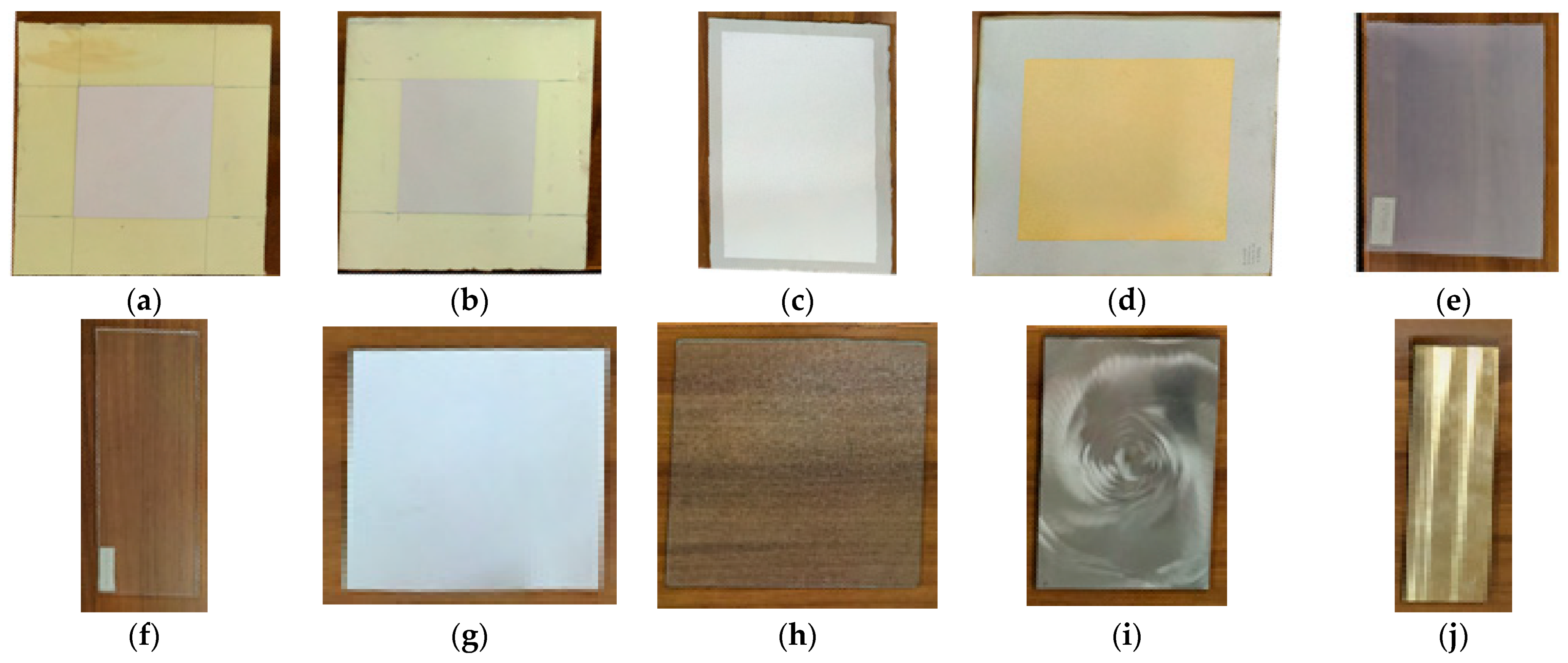
| Sample Material | Dimensions [m] | Area [sqm] | Albedo |
|---|---|---|---|
| Smooth cement plaster | 0.4 × 0.45 × 0.05 | 0.180 | 0.514 |
| Raw cement plaster | 0.4 × 0.45 × 0.05 | 0.180 | 0.524 |
| White lime plaster | 0.505 × 0.365 × 0.01 | 0.184 | 0.518 |
| Coloured lime plaster | 0.525 × 0.47 × 0.01 | 0.247 | 0.510 |
| Tetrafluoroethylene (TFE) | 0.245 × 0.19 × 0.001 | 0.046 | 0.455 |
| Methacrylate (PMMA) | 0.305 × 0.12 × 0.005 | 0.037 | 0.433 |
| High-density polyethylene (HDPE) | 0.23 × 0.22 × 0.002 | 0.051 | 0.623 |
| Frosted glass | 0.3 × 0.3 × 0.005 | 0.090 | 0.517 |
| Steel | 0.205 × 0.3 × 0.008 | 0.061 | 0.606 |
| Brass | 0.105 × 0.303 × 0.009 | 0.032 | 0.661 |
| Resolution | R2 for Scanning Distance: 0.5 m | R2 for Scanning Distance: 1.5 m |
|---|---|---|
| 1 cm (iOS) | 0.54 | 0.68 |
| 1.5 cm (iOS) | 0.53 | 0.40 |
| 2 cm (Android) | 0.27 | 0.20 |
| Object Scanned | Scan Distance: 2 m | Scan Distance: 3 m | ||
|---|---|---|---|---|
| Statue | SVλ 1.5 cm | SVλ 2 cm | SVλ 1.5 cm | SVλ 2 cm |
| 0.0071 | 0.0103 | 0.0417 | No data | |
| Oλ 1.5 cm | Oλ 2 cm | Oλ 1.5 cm | Oλ 2 cm | |
| 0.0012 | 0.0013 | 0.0017 | No data | |
| Object Scanned | Scan Distance: Adaptative | ||
|---|---|---|---|
| Laboratory room | SVλ 1 cm | SVλ 1.5 cm | SVλ 2 cm |
| 0.0119 | 0.0109 | 0.0234 | |
| Pλ 1 cm | Pλ 1.5 cm | Pλ 2 cm | |
| 0.8607 | 0.8940 | 0.7849 | |
| Object Scanned | Scan Distance: Adaptative | ||
|---|---|---|---|
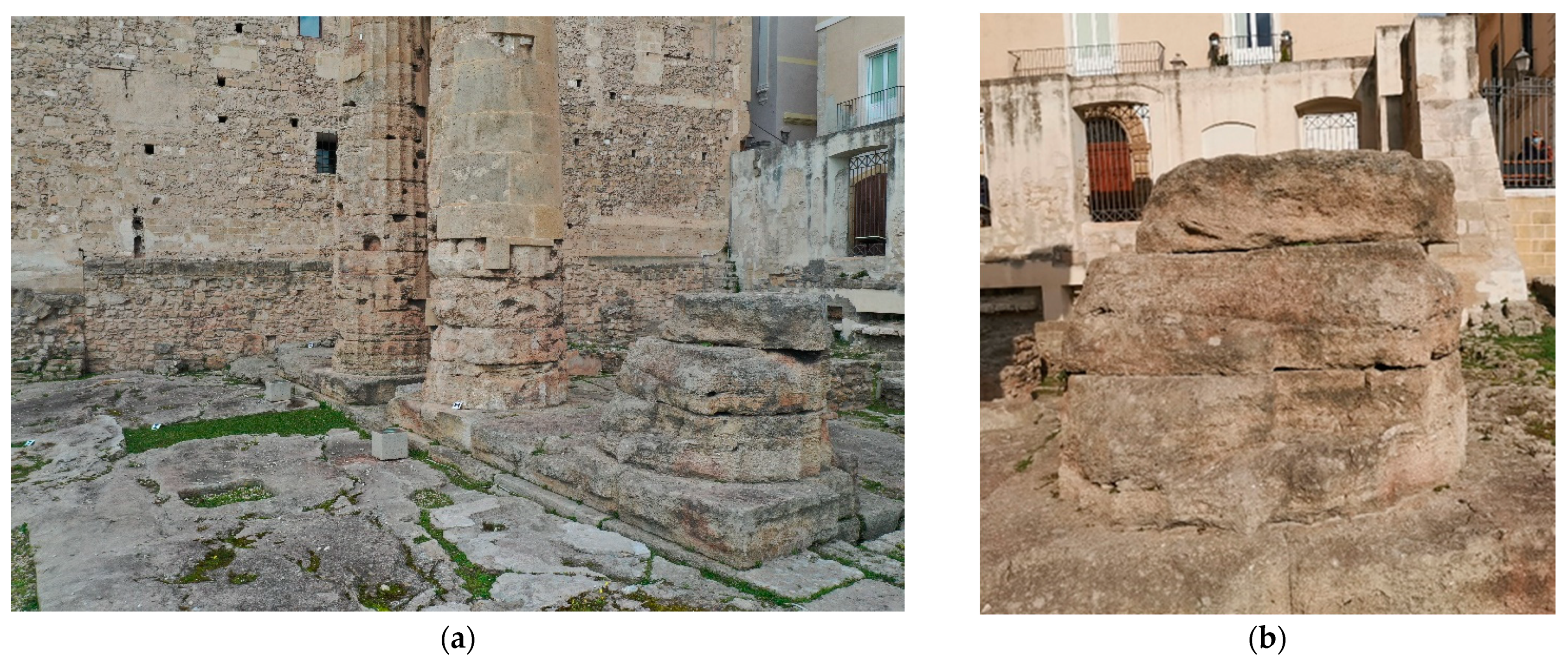
| Doric column rests | SVλ 1 cm | SVλ 1.5 cm | SVλ 2 cm |
| 0.0400 | 0.0682 | 0.0309 | |
| Oλ 1 cm | Oλ 1.5 cm | Oλ 2 cm | |
| 0.0019 | 0.0022 | 0.0018 | |
| Object Scanned | Resolution: 1 cm | Resolution: 1.5 cm | Resolution: 2 cm | |||
|---|---|---|---|---|---|---|
| µ C2C [m] | σ C2C [m] | µ C2C [m] | σ C2C [m] | µ C2C [m] | σ C2C [m] | |
| Laboratory room | 0.0334 | 0.0264 | 0.0224 | 0.0449 | 0.0518 | 0.0580 |
| Doric column rests | 0.0153 | 0.0132 | 0.0383 | 0.0238 | 0.0127 | 0.0107 |
Publisher’s Note: MDPI stays neutral with regard to jurisdictional claims in published maps and institutional affiliations. |
© 2022 by the authors. Licensee MDPI, Basel, Switzerland. This article is an open access article distributed under the terms and conditions of the Creative Commons Attribution (CC BY) license (https://creativecommons.org/licenses/by/4.0/).
Share and Cite
Costantino, D.; Vozza, G.; Pepe, M.; Alfio, V.S. Smartphone LiDAR Technologies for Surveying and Reality Modelling in Urban Scenarios: Evaluation Methods, Performance and Challenges. Appl. Syst. Innov. 2022, 5, 63. https://doi.org/10.3390/asi5040063
Costantino D, Vozza G, Pepe M, Alfio VS. Smartphone LiDAR Technologies for Surveying and Reality Modelling in Urban Scenarios: Evaluation Methods, Performance and Challenges. Applied System Innovation. 2022; 5(4):63. https://doi.org/10.3390/asi5040063
Chicago/Turabian StyleCostantino, Domenica, Gabriele Vozza, Massimiliano Pepe, and Vincenzo Saverio Alfio. 2022. "Smartphone LiDAR Technologies for Surveying and Reality Modelling in Urban Scenarios: Evaluation Methods, Performance and Challenges" Applied System Innovation 5, no. 4: 63. https://doi.org/10.3390/asi5040063