
Universal Behavior of the Image Resolution for Different Scanning Trajectories

1
Department of Robotics, School of Engineering and Digital Sciences, Nazarbayev University, Astana 010000, Kazakhstan
2
Department of Physiology and Biomedical Engineering, Mayo Clinic, Scottsdale, AZ 85259, USA
3
Department of Biology, School of Sciences and Humanities, Nazarbayev University, Astana 010000, Kazakhstan
*
Authors to whom correspondence should be addressed.
Appl. Syst. Innov. 2023, 6(6), 103; https://doi.org/10.3390/asi6060103
Submission received: 23 August 2023
/
Revised: 17 October 2023
/
Accepted: 23 October 2023
/
Published: 2 November 2023
Abstract
:This study examines the characteristics of various scanning trajectories or patterns under the influence of scanning parameters in order to develop a theory to define their corresponding image resolutions. The lack of an accurate estimation of pixel size for a specified set of scanning parameters and their connection is a key challenge with existing scanning methods. Thus, this research aimed to propose a novel approach to estimate the pixel size of different scanning techniques. The findings showed that there is a link between pixel size and a frequency ratio , which is the ratio of two waveform frequencies that regulates the density of the scanning pattern. A theory has been developed in this study to explain the relationship between scanning parameters and scanning density or pixel size, which was not previously considered. This unique theory permitted the a priori estimate of the image resolution using a particular set of scanning parameters, including the scan time, frequencies, frequency ratio, and their amplitudes. This paper presents a novel and systematic approach for estimating the pixel size of various scanning trajectories, offering the user additional flexibility in adjusting the scanning time or frequency to achieve the desired resolution. Our findings also reveal that in order to achieve a high-quality image with high signal-to-noise and low error, the scanning trajectory must be able to generate a fairly uniform or regular pattern with a small pixel size.
1. Introduction
Nowadays, scanning techniques are gaining popularity and becoming an essential component of a variety of devices, including microelectromechanical systems (MEMS), light detection and ranging (LiDAR) [1], atomic force microscopy (AFM) [2], magnetic resonance imaging (MRI) [3,4,5,6], and magnetic particle imaging (MPI) [7,8,9,10,11], mapping and surveying mechanisms [12], and frequency modulated gyroscopes [13].
Due to its great performance and low cost, MEMS LiDAR is quickly becoming an essential sensor in vehicle environment sensing systems. The LiDAR method can be used in many different areas, such as agriculture [14], autonomous vehicles [15], and drones [16].
The three main technologies of MEMS LiDAR imaging are the beam-scanning trajectory, sampling scheme, and gridding. In order to obtain a denser scanning trajectory or pattern in a specific field of view (FOV) at the same scanning frequency, the sampling scheme should be enhanced. A universal sampling strategy that is unrelated to the beam scanning trajectory patterns is suggested by summarizing the laws of the Cartesian grid. Image resolution and the number of points per frame are both doubled compared to the already utilized sampling scheme with the same hardware setup and scanning frequency for the MEMS scanning mirror (MEMS-SM). This is advantageous for enhancing MEMS LiDAR’s point cloud imaging capability [17].
Atomic force microscopy (AFM) has traditionally used triangular or saw-tooth signals for raster scanning. While this technology can offer workable answers during slow processes, it cannot provide adequate solutions during rapid scan regimes. High-speed atomic force microscopy is gaining popularity, especially for studying the dynamic behavior of biological molecules or their interactions with light. The raster-signal frequency is normally restricted to 1% of the first-resonance frequency of the positioning stage for an acceptable performance in traditional raster scanning. This restriction guarantees adequate monitoring of the raster signal’s high-order harmonics while preventing the stage’s vibration modes from being activated. As a result, the scan speed is slow, and it takes longer to completely scan the FOV of interest. Furthermore, in a highly resonant stage, monitoring sinusoidal reference signals with a narrow bandwidth is easier than tracking triangle or saw-tooth references at the same amplitude and fundamental frequency. Non-raster approaches, such as the Lissajous scanning trajectory, can be used instead of raster scanning to produce high-quality images at high scan rates [18].
Scanning trajectories are also used by medical imaging techniques like MRI [3,4,5,6] and MPI [7,8]. These imaging methods are essential because they can be used to look inside the human body without undergoing surgery and to diagnose, monitor, prevent, and treat a variety of diseases [19]. The purpose of these techniques is to scan the FOV to obtain an image that will be used later to analyze the patient’s condition. The type of scanning trajectory chosen is crucial for obtaining accurate results. By choosing the appropriate or optimal trajectory, scanning time can be reduced and image quality can be enhanced in order to make an accurate diagnosis. This implies that a proper scanning trajectory can be very important for patient diagnosis and care [20].
It should be emphasized that all of the aforementioned methods are currently in the development stage, meaning that researchers are trying to improve them. Although the field is expanding, a fundamental problem with the present scanning techniques is the lack of a reliable estimation of the pixel size for a particular combination of scanning settings. For example, it is currently unknown what the pixel size of this scan will be given a chosen scanning trajectory to scan a FOV with a particular set of scanning parameters. Keep in mind that the quality of the reconstructed image from the scan is directly impacted by the choice of pixel size. Thus, understanding every aspect of the scanning pattern within the FOV, including the scanning pattern density, the time spent, the signal-to-noise ratio, and the error in each local region, is absolutely essential. It is crucial to consider the importance of the appropriately quantified pixel size or the empty gap between the pattern and its distribution within the FOV. Here, it is important to distinguish between the ideas of image resolution and spatial resolution. Image resolution is primarily determined by the total number of pixels in an image, which is also defined by the size of each pixel in that image. For instance, a fixed size image with many small pixels rather than a few large pixels will have a high image resolution. Hence, image resolution is inversely proportional to pixel size. The amount of detail and sharpness visible in the image is determined by the image resolution. In contrast, spatial resolution refers to the smallest discernible detail in an image, which establishes the level of detail that an imaging system, such as a camera or sensor, is able to differentiate. Spatial resolution is typically expressed by the smallest resolvable feature size, which can be measured in millimeters, micrometers, or even nanometers. In general, to distinguish fine details in an image, the image resolution must be greater than the spatial resolution (i.e., the size of the pixel must be a few folds smaller than the spatial resolution) [21]. As a result, the main emphasis of this paper is on the image resolution generated by different scanning trajectories and how it is related to the selection of scanning parameters.
Any trajectory scanning system has a scanning point that sweeps through the FOV in a particular pattern [6,22]. The image resolution, scan time, or speed may vary depending on the trajectory selected, which can also affect the quality of the to-be-scanned images [8]. Thus, being able to measure image resolution through the pixel size and understand how it relates to the scanning parameters is crucial, especially for the system operators [23]. The primary objective of this work is to establish a theory for determining the minimal image resolution, or maximum pixel size, using all of the trajectory crossing points (indicated by the blue dots on all scanning patterns shown in Figure 1) throughout the whole FOV. The image resolution and its impact on the quality of the reconstructed image are also evaluated for a variety of trajectories that can be utilized in biomedical imaging. There are various scanning trajectories available these days, which include bidirectional Cartesian (BC), triangular Lissajous (TL), sinusoidal Lissajous (SL), radial Lissajous (RL), unidirectional Cartesian, Cartesian improved, spiral, and radial. This paper will concentrate on the first four scanning trajectories, namely BC, TL, SL, and RL, due to their high scan resolution, fairly regular pattern formation, and ability to generate quality reconstructed images with isotropic resolution [8,24].
To fulfill the aforementioned goals, the following section will first focus on determining the maximum pixel size for all scanning trajectories for a variety of scanning parameters. The relationship between pixel size and scanning parameters will then be established. The effect of scanning parameters on pixel coverage will be investigated next. Finally, the effectiveness and accuracy of image reconstruction for all trajectories will be assessed and compared.
2. Scanning Methods
2.1. Scanning Trajectory Pattern and Density
To comprehend the relationship between image resolution and scanning trajectory, it is necessary to first define the pixel size of any scanning trajectory. Pixel size can be defined as the half of the shortest distance between two non-overlapping scanning lines that are usually parallel to each other [25]. Let us first identify and utilize the coordinate position of crossing sites by which two scanning lines overlap as reference points; these points are represented by the blue dots in Figure 1. Depending on the scanning patterns, these crossing points divide the image into either a uniform or non-uniform grid. The patterns created by Cartesian (Figure 1a) and non-Cartesian (Figure 1b–d) scanning paths and their overlapping sites are shown in Figure 1. It can be seen here that for each crossing point that is not on the boundary, the closest six neighboring points are those that set the minimum () and maximum () distances between this crossing point and those belonging to its next adjacent lines (see Figure A1 in Appendix A for a zoomed in version of all trajectories).
Distances between each crossing point and its six nearest neighbors in the FOV are first calculated and sorted to obtain the (shown by the red dashed line) and (indicated by the green dashed line) values [24]. The pixel size of the scanning pattern should at least be established using the value with the greatest minimum distance because each crossing point has its own and values. In general, each crossing point should have eight nearest neighbors; however, the final two farthest next nearest neighbor points are not required for calculating the image resolution. This is because the shortest distance between the two parallel nearest neighbor lines will always be used to determine the pixel size, and, hence, image resolution.
Despite the fact that and are straightforward definitions of distances that nearly approximate the pixel size, they do not precisely depict the true pixel size of the scanning pattern. In reality, a considerably more precise representation that is usually employed to identify the pixel size is the largest/longest perpendicular distance between two contiguous scanning lines in the FOV, represented by in Figure 1 [25]. To calculate at each crossing point, the largest perpendicular distance from the focus/center crossing point to all nearest adjacent scanning lines are calculated. and are required to calculate . Two to four were acquired depending on the irregularity of the scanning trajectory, and they were sorted to achieve the highest value of . In other words, the values of depend on the scanning trajectory and can be either four distinct values or two couples of values.
The maximum value of , , and for all points in the FOV are recorded because these values closely represent the pixel size, especially the . This method of calculating the pixel size eliminates the risk of underestimating or overestimating the image resolution, which would occur if the average values of all estimated distances within the FOV were used.
A theoretical formulation for , , and does not exist for the majority of scanning trajectories. Fortunately, it is possible to make theoretical predictions of and for the sinusoidal Lissajous, which are provided below [25]:
where and are the width and height of the FOV, while and represent the number of lobes or stripes along the x and y axes, respectively. Equations (1) and (2) above clearly show that if the FOV is fixed, and depend on the number of lobes and . As a result, given a fixed FOV, increasing the lobe count will result in a denser pattern, and, hence, a higher image resolution.
An earlier investigation into the sinusoidal Lissajous trajectory revealed that a configuration of = = will guarantee the highest density of the forming pattern [26]. Here, is the ratio of two frequencies of the x and y axes, and , and it is proportional to the scanning density or image resolution (see Table 1 for more details). Trajectory-scanning patterns are usually generated from the conjunction of two signals. The waveforms are typically sinusoidal signals with variable frequencies ( and ) and amplitudes (A and B). The shape and density of the scanning trajectory can vary depending on the value of . Table 1 provides a summary of the full definitions for these parameters and coefficients. Although there are theoretical formulas for and for the sinusoidal Lissajous trajectory, there is not one for [25]. However, our work indicates that the values of and are required to determine . Therefore, in the majority of situations, these numbers will need to be determined numerically.
In terms of the selection of trajectories, this work will concentrate on the four primary trajectories: bidirectional Cartesian (BC), triangular Lissajous (TL), sinusoidal Lissajous (SL), and radial Lissajous (RL), which are frequently utilized for MPI research. The formulation and characteristics of these trajectories are presented in Table 1 ((3)–(10)).
2.2. Scanning Trajectory Characteristics
Unlike the unidirectional Cartesian trajectory, the BC trajectory propagates in both directions, as seen in Figure 1a. BC is the trajectory in the Cartesian family that has the highest resolution [24]. Compared to sinusoidal and triangular approaches, the resolution and regularity are lower. Moreover, the image reconstruction with BC scanning is also challenging [7].
The waveforms that make up the TL trajectory are both triangular and saw-tooth. It is created by combining two distinct triangular signals, each with a different frequency [26]. Despite the TL trajectory being quite uniform and homogeneous throughout the FOV, as observed in Figure 1b, the image resolution produced is not better than the SL trajectory [7,8].
SL is a non-Cartesian sinusoidal scanning trajectory that provides acceptable scanning duration and resolution (Figure 1c). The irregularity of the forming pattern is the primary disadvantage of this trajectory, particularly in the center of the FOV where large gaps are located. As a result, this trajectory not only exhibits an uneven distribution of scanning density and image quality, but it also has low resolution in the FOV’s center [29].
RL is another non-Cartesian sinusoidal scanning trajectory with an extremely dense center and moderately dense borders. Depending on the amplitude values selected, the trajectory has an elliptic or circular shape, as implied by its name. RL is a member of the Lissajous family, and its trajectory formulas are similar [24].
In this study, was set to 25 kHz for all cases, and the FOV was set to be 3.2 cm long by 1.6 cm wide [8]. Changes in image resolution within the field of view can be observed by adjusting . In other words, a higher number of denotes a denser pattern within the FOV.
3. Results and Discussion
3.1. Scanning Patterns
Figure 1a–d illustrate the scanning patterns formed by different trajectories. While the TL is regular and values of , , and do not change, the BC, SL, and RL have different , , and values over the FOV. The pattern produced by SL is denser at the edges and sparser in the middle [30]. Its regularity is better than BC but is not as regular as TL. RL does not scan the entire FOV, producing a pattern that is very dense in the center and moderately dense near the edges. The BC scan trajectory has the lowest regularity and resolution when compared to other scanning trajectories.
Figure 2a,b depict the relationship between the maximum distance and as a function of , respectively. As can be seen, theoretical and numerical values agreed quite well. The inset shows the same plot with both the x and y axes displayed in log10 format. The log–log plot of the data clearly shows that and display a hyperbola, with the values decreasing as increases. Our results support previous estimates that for large values of , and of the SL trajectory are proportional to the reciprocal of [18,25].
The density of the scanning pattern for = 100 has been proven to be sufficient for producing a good-quality image [8,24]. Therefore, the pixel size of the phantom image to be utilized for image reconstruction in this work will be determined using the pixel size of this value. Table 2 displays the numerically determined values of , , and for all four types of scanning trajectories at = 100.
3.2. Relationship between Pixel Size and Scanning Parameters
To understand the relationship between pixel size and for all four scanning trajectories, numerical calculations are performed to estimate values of , , and for values ranging from 10 to 400.
Because the maximum values of and exhibit a hyperbola function of for the SL trajectory, it is safe to assume that this trend will also hold for and all remaining trajectories investigated in this work. Figure 3a–d display the trend of , , and as a function of for all four scanning techniques examined in this work. Here, we can see that also follows the same trend as and . The figure also demonstrates that for all scanning trajectories, numerically computed values for , , and fit well to a hyperbola, specified in (11). The obtained values, which are almost unity, further support the quality of the fit. The percentage of variation in dependent variables that can be explained by the independent variable is shown statistically by the coefficient, also known as the coefficient of determination. In other words, the result is a measurement of how well the data fit the model, and a value close to unity indicates a near perfect match. The variation in values across all trajectories is depicted in Figure 3e. As can be seen at a particular value of , RL has the lowest value, which is then followed by SL, TL, and then BC.
where and are constants.
It is important to note that the BC scanning trajectory formula that is currently in use is incomplete. This equation only performs well when /2 is even. For all /2 is odd cases, the scanning pattern is discontinuous at the haft-way point of the repetition time. This means that the BC trajectory formulas presented in (3) and (4) are only relevant in /2 even cases (Figure A2 in Appendix A shows trends for both even and odd /2 cases). Here, we can observe that the trend of distance value for odd cases is slightly larger than for even situations, showing that the formulation for odd and even circumstances is inconsistent. Only numerically generated values for /2 that are even are utilized in this work to ensure the consistency and accuracy of the computed data for the BC trajectory.
The values of the constants and that were determined by fitting the data to (11) are listed in Table 3. It should be noted that the values for are close to unity for all trajectories. Our results demonstrated that all of the defined distances , , and for the four scanning trajectories examined in this work are proportional to . The findings showed that the inversely proportional relationship between the distance or pixel size and is a common characteristic of all the analyzed trajectories, not just the sinusoidal Lissajous trajectories. Thus, setting the value of to unity further simplified the formulas for , , and . Substituting this to (11) yields:
Equation (12) states that is inversely proportional to the pixel size, which is determined by a value from either , , or . This means that as increases, the pixel size decreases, resulting in an improvement in image resolution or image quality. Table 4 shows the updated values of that were determined by the fit when a = 1. It should be noted that new values remain very close to 1 after setting a = 1, indicating a high-quality fit.
Note that is related to the scanning frequency and the repetition time via the following formula [8]:
Substituting (13) into (12) leads to the following equation:
Equation (13) shows that the scanning duration is directly related to , whereas the coefficient is inversely proportional to the scanning trajectory’s resolution. Combining these connections yields (14), which demonstrates that the frequency and repetition time are inversely related to the scan resolution. Such kinds of relationships between imaging parameters were not previously mentioned; thus, it is crucial and significantly important to be able to analyze the data.
3.3. Scanning Pixel Coverage
The fill factor (FF) is one metric used to gauge how well scanning procedures are working. It measures the proportion of active pixels to all pixels. The pixels that the scanning trajectory covered or touched are referred to as active pixels in this context. In other words, if the scan’s trajectory passes over a pixel, that pixel is considered active. The FF is expressed as a percentage, where 100% corresponds to complete coverage of all the pixels in the FOV by the scanning trajectory.
The pixel size was estimated by the of each case, as it is known that the number of pixels in each FOV was chosen by dividing the width and height to half of the to accurately represent the image. For example, Figure 4a shows the FF for different scanning trajectories assessed using the BC pixel size for various values ranging from 10 to 400.
According to Figure 4a–d, the highest fill factor among the four mentioned trajectories is RL. This trend was expected due to the dense pattern formed by the RL scanning trajectory. However, one of the main drawbacks of RL is that it scans only the center circular/elliptical area of the FOV. This makes it inappropriate for scanning rectangular/square areas, like in our case.
3.4. Image Reconstruction
The image was then reconstructed using all of the investigated scanning trajectories [31]. MPI is one of the primary uses of the aforementioned scanning methods. As a result, additional analysis will be carried out utilizing image reconstruction in MPI. System matrix method was used to reconstruct the image. This method is preferred because it may be used for any type of trajectory.
The phantom was designed to be 3.2 cm wide and 1.6 cm tall, with the supposed word “NU” filled with super paramagnetic iron oxide nanoparticles (SPION) (see Figure 5a). In order to guarantee a high fill factor for all trajectories, the Nyquist–Shannon sampling theorem was used, with a pixel size set at half of . Table 5 contains some of the factors that were used to perform the image reconstruction using the system matrix method.
As previously stated, the number of pixels in each side length of the phantom was determined by dividing the phantom’s width and height by . Thus, as the decreases, the number of pixels represents an image increase. We chose to perform image reconstruction for all four scanning trajectories using the value of the BC trajectory because this value ensures that all trajectories have a fill factor of at least 90%. Using different mesh sizes that reduce the fill factor for some trajectory to less than 90% may produce bias in the reconstruction as well as the quality for a fair comparison. Figure 5b depicts the reconstructed image obtained by utilizing the value for the BC scanning trajectory. The reconstructed image using the value of the SL scanning pattern is shown in Figure A3 in Appendix A.
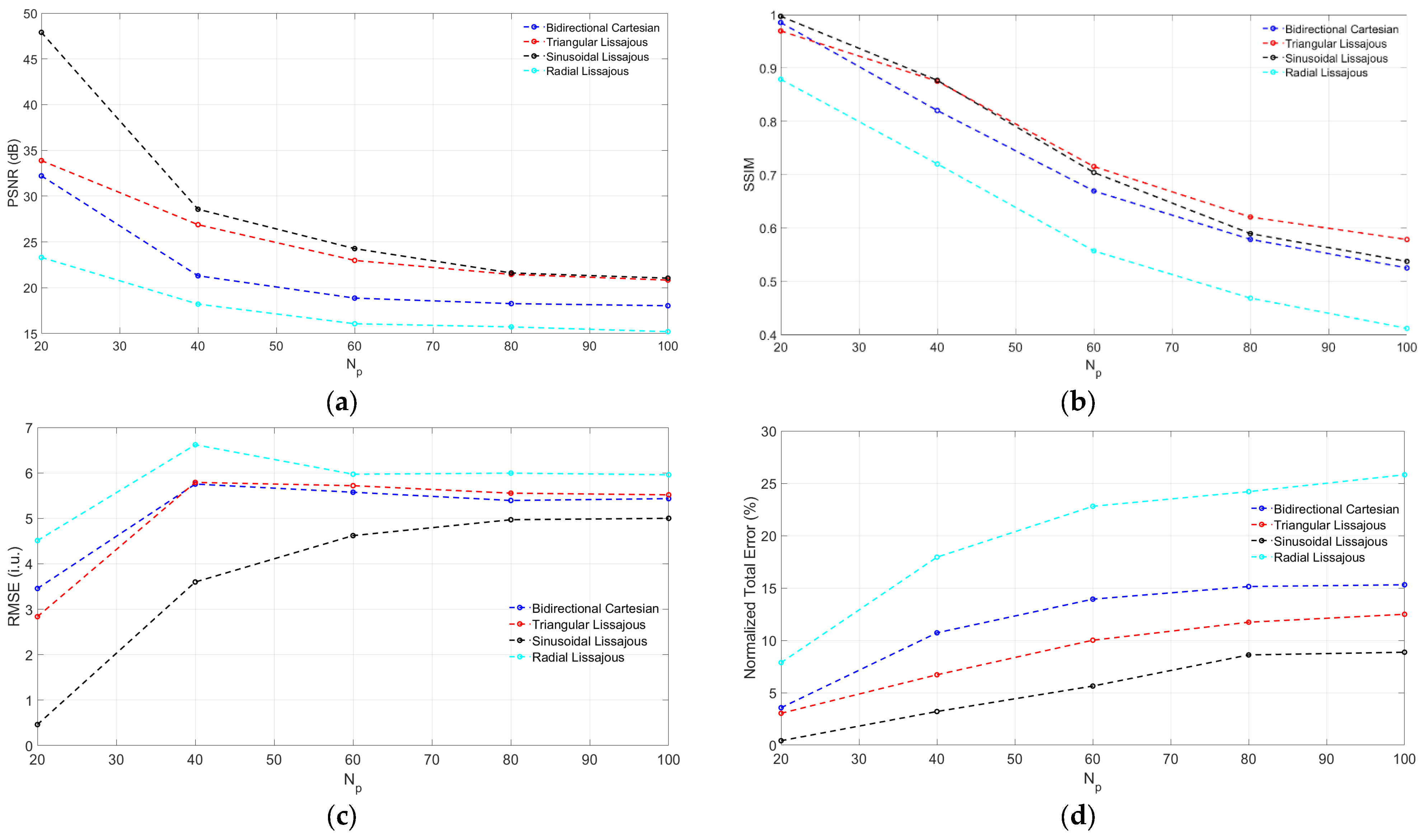
To assess the similarity between the reconstructed and phantom images, the peak signal-to-noise ratio (PSNR) is used [32]:
Here, represents the intensity unit of the reconstructed image, while represents the intensity unit of the phantom. The unit of PSNR is in decibels (dB). A high PSNR score indicates that the reconstructed image is comparable to the phantom image. Figure 6a depicts the estimation of PSNR for image reconstruction of all scanning trajectories using the BC mesh.
Another metric for quantifying the degree of accuracy of the reconstructed image is the structural similarity index measure (SSIM), which measures the similarity between two images. The SSIM is defined as follows [33,34,35,36]:
where and are the mean over a window in Image X and Image Y, respectively. and are the standard deviation over a window in Image X and Image Y. is the co-variance over a window between Image X and Image Y and and are constants. Figure 6b illustrates the values of SSIM for all scanning trajectories.
In order to quantify the quality of the reconstructed image, it is also important to quantify the error. The formula for calculating the Root Mean Square Error (RMSE) is as follows [37,38,39]:
Figure 6c shows the RMSE of various scanning methods calculated using (16) above. The Normalized Total Error (NTE) is another approach for quantifying the error, and it is defined as [40]:
The NTE for various scanning methods as a function of was calculated and illustrated in Figure 6d. It is important to note that the NTE is expressed as a percentage rather than an intensity unit like the RMSE.
For the BC trajectory, it should be noted that this pattern is not as dense, and it has a larger compared to other trajectories. This means that this scanning technique detects less signal than others (refer to Table 2). Figure 6a,b depict the trend of the PSNR and SSIM for all trajectories, demonstrating that the value is highest when is lowest but decreases when increases. This is because the size of the BC mesh is shrinking and becoming more difficult to detect. As can be seen in Figure 6c,d, the RSME and NTE levels start out being low but rise as increases, plateauing at a large . In general, the trends of PSNR/SSIM and RMSE/NTE are inverse, which means that when the error is low, PSNR and SSIM must be high, and vice versa. Despite the fact that the mesh was created using the BC method and the FF value is greater than 90% for all conditions, this BC scanning technique shows poor results in terms of reconstruction. The primary cause of this is the formation of the pattern from this trajectory, which is quite sparse and incapable of accurately detecting the objects.
Among the methods already described, the TL trajectory has the most consistent and regular pattern. Unfortunately, although having a regular pattern, the image resolution is lower (i.e., value is larger) than the SL and RL trajectories (see Table 2), which results in a lower-quality reconstructed image.
Figure 6a,b clearly demonstrate that the PSNR and SSIM values for the SL trajectory are comparable to the TL, and Figure 6c,d show that the values of RMSE and NTE are lower than those of other scanning techniques. This proves that the most appropriate technique for reconstruction of this NU phantom is the SL trajectory. Similar findings are obtained for the SL mesh (see Figure A4 in Appendix A), demonstrating that SL is the best scanning trajectory for generating high signal-to-noise and low error for image reconstruction. Our results confirmed previously reported findings that the SL trajectory is superior to most other trajectories because it produced excellent image quality even at low scanning densities [8,24].
Surprisingly, compared to the other trajectories, the RL produced the greatest RMSE and NTE values while attaining the lowest PSNR and SSIM values, which resulted in the worst reconstruction outcomes (see Figure 5 and Figure 6). According to Table 2 and Figure 3e, RL has the lowest . However, it does not scan the corners of the FOV, as seen in Figure 1d. This could result in an increase in the RSME and NTE values at the corners of the image along with a decrease in the PSNR and SSIM. Additionally, the BC, SL, and RL trajectories all have the same repetition time. This means that for a trajectory with a much denser scanning pattern, the time spent continuously resting on the pixel is substantially less, but with a greater frequency. As a result, the short visit of the scan on the pixel may result in a lower signal-to-noise ratio and a higher error. Similar results have been observed concerning the quality of images generated by confocal microscopes, where the pixel scanning duration or pixel dwell time primarily controls the signal-to-noise ratio rather than the frequency of scans. Thus, a scanning trajectory that produces a very dense and/or irregular pattern, such as the RL, may not be the best choice due to frequent but very short visits of the pixels, which has a detrimental impact on reconstruction outcomes.
These findings seem to suggest that the scanning trajectory’s density or pixel size is not the main factor that leads to an accurate reconstruction of the true image. The data clearly demonstrate the inverse correlation between similarity (PSNR and SSIM) and error (RMSE and NTE). The regularity and pixel size of the scanning pattern have a significant impact on the quality of the reconstructed image. Our findings imply that the scanning trajectory needs to generate a fairly regular pattern as well as a small pixel size in order to produce a high-quality reconstructed image.
4. Conclusions
This study attempted to establish a correlation between image resolution and scanning parameters by investigating the characteristics of different scanning trajectories, such as pixel size, fill factor, scan time, frequency, and frequency ratio. Our findings suggested that the pixel size and the frequency ratio of the scanning trajectory have a straightforward relationship. More specifically, and the pixel size formed by the scanning trajectory investigated in this work are inversely related. This relationship holds true across all scanning trajectories investigated in this work and is universal. The research produced a theory to explain the previously neglected correlation between scanning parameters and pixel size, which determines image resolution. The proposed theory can serve as a foundation for the correlation between image resolution and a number of variables, including scan time, fundamental frequency, and frequency ratio . The work also provides a novel method for estimating the pixel size a priori, giving the user/operator more control over how to modify the scanning parameters for a desired resolution. Image reconstructions were also performed for all scanning trajectories. Our results indicated that SL is the preferred trajectory because it produced the best image quality with high signal-to-noise and low error when compared to other trajectories. Our findings also suggest that a good scanning trajectory for producing high-quality images is one that can produce a highly regular pattern and small pixel size. The findings from this study can be utilized to improve the effectiveness and quality of scanning images in a variety of real-world scenarios, such as topological mapping, heat mapping, and water mapping for LiDAR-based area surveillance as well as MPI and AFM imaging for biological and biomedical applications.
Author Contributions
A.M. performed simulations, data analysis, and manuscript preparation. T.-A.L. assisted in the theory development and image reconstruction. T.D.D. and T.T.P. secured funding and conceptualized, designed, and directed the project, wrote codes, supervised, and wrote—review and editing. All authors have read and agreed to the published version of the manuscript.
Funding
This work was supported by Nazarbayev University under the Faculty Development Competitive Research Grant Program (FDCRGP), Grant No. 11022021FD2924 (TDD) and 021220FD4451 (TTP).
Data Availability Statement
Data is available upon request.
Conflicts of Interest
The authors declare no conflict of interest.
Appendix A
Figure A1.
Zoomed-in view of the distance to the nearest adjacent neighbors for different waveforms with the nearest (red dashed lines) and farthest (green dashed lines) distances and the maximum value for = 12 for (a) bidirectional Cartesian, (b) triangular Lissajous, (c) sinusoidal Lissajous, and (d) radial Lissajous.
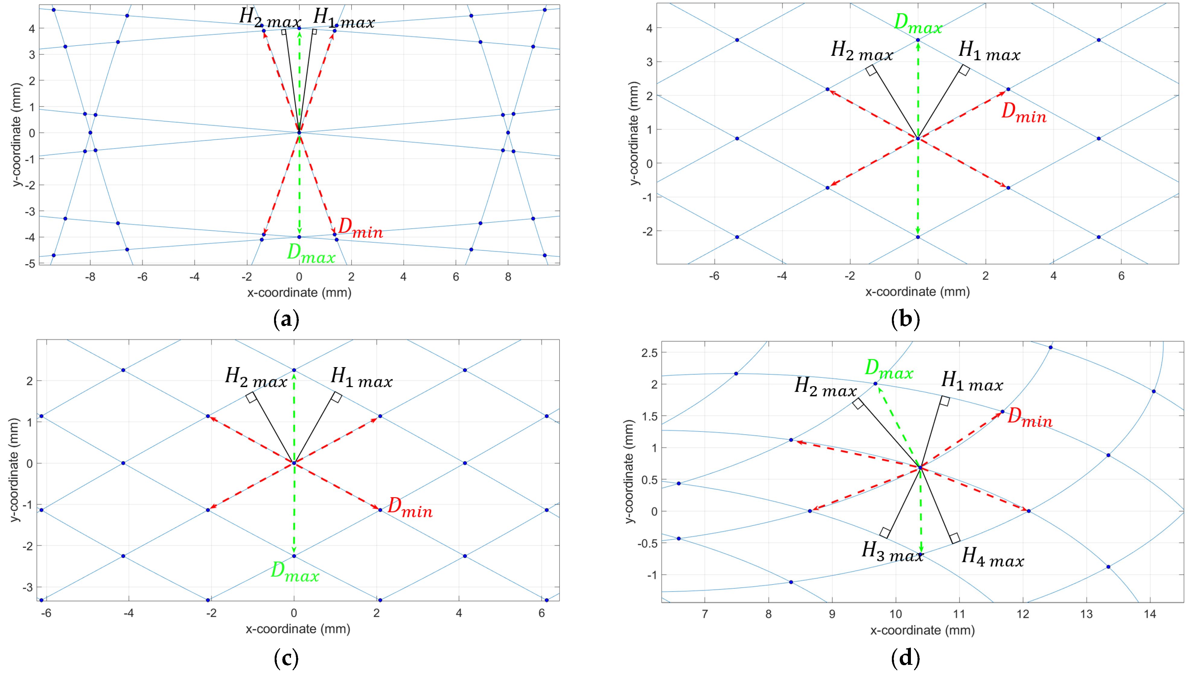
Figure A2.
The regression line for the spatial separation of bidirectional Cartesian scanning trajectory for both /2 is odd and /2 is even.
Figure A2.
The regression line for the spatial separation of bidirectional Cartesian scanning trajectory for both /2 is odd and /2 is even.
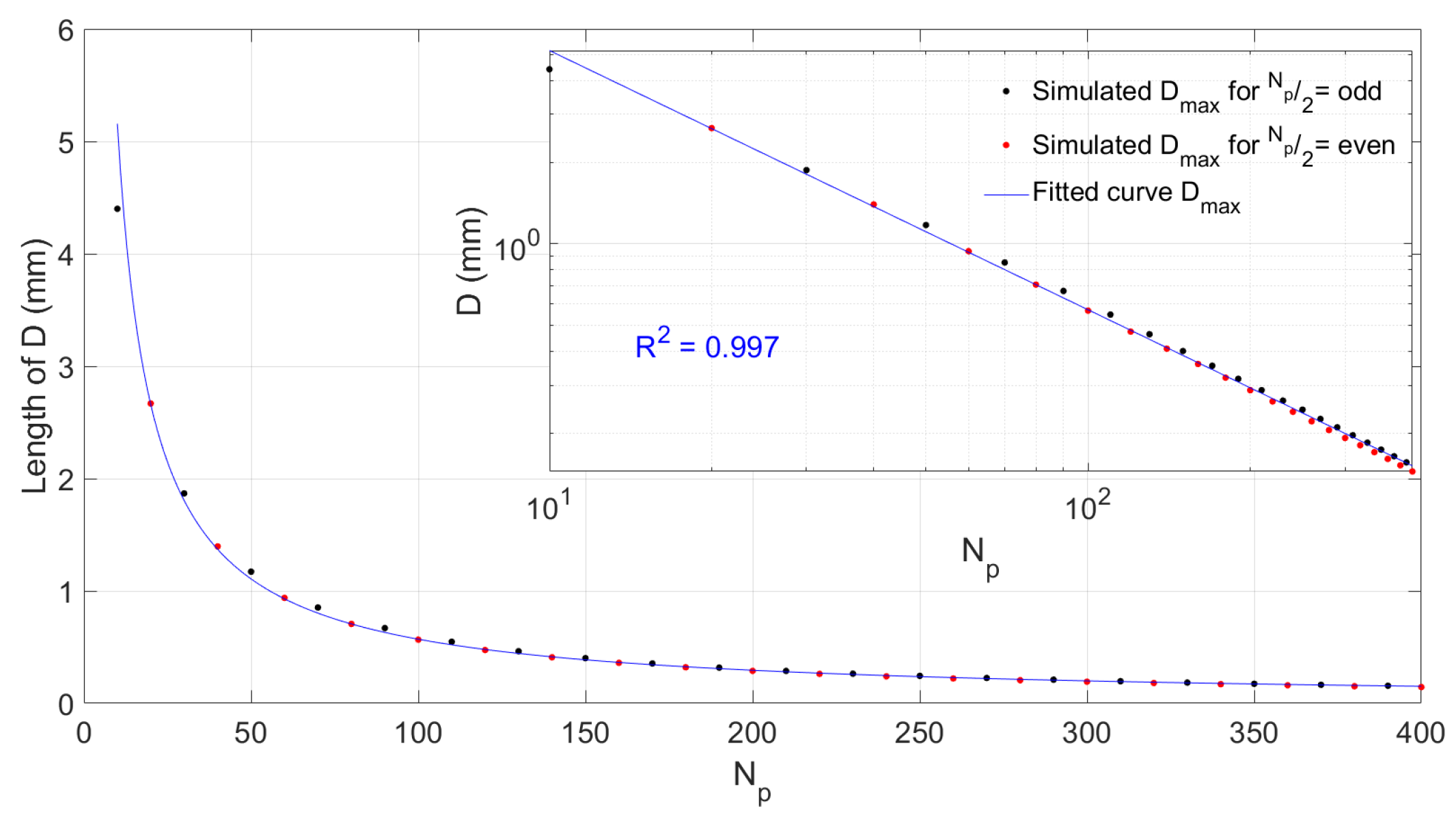
Figure A3.
Results of the reconstructed images using sinusoidal Lissajous mesh ( value of SL was used as the pixel size) for various scanning patterns and .
Figure A3.
Results of the reconstructed images using sinusoidal Lissajous mesh ( value of SL was used as the pixel size) for various scanning patterns and .
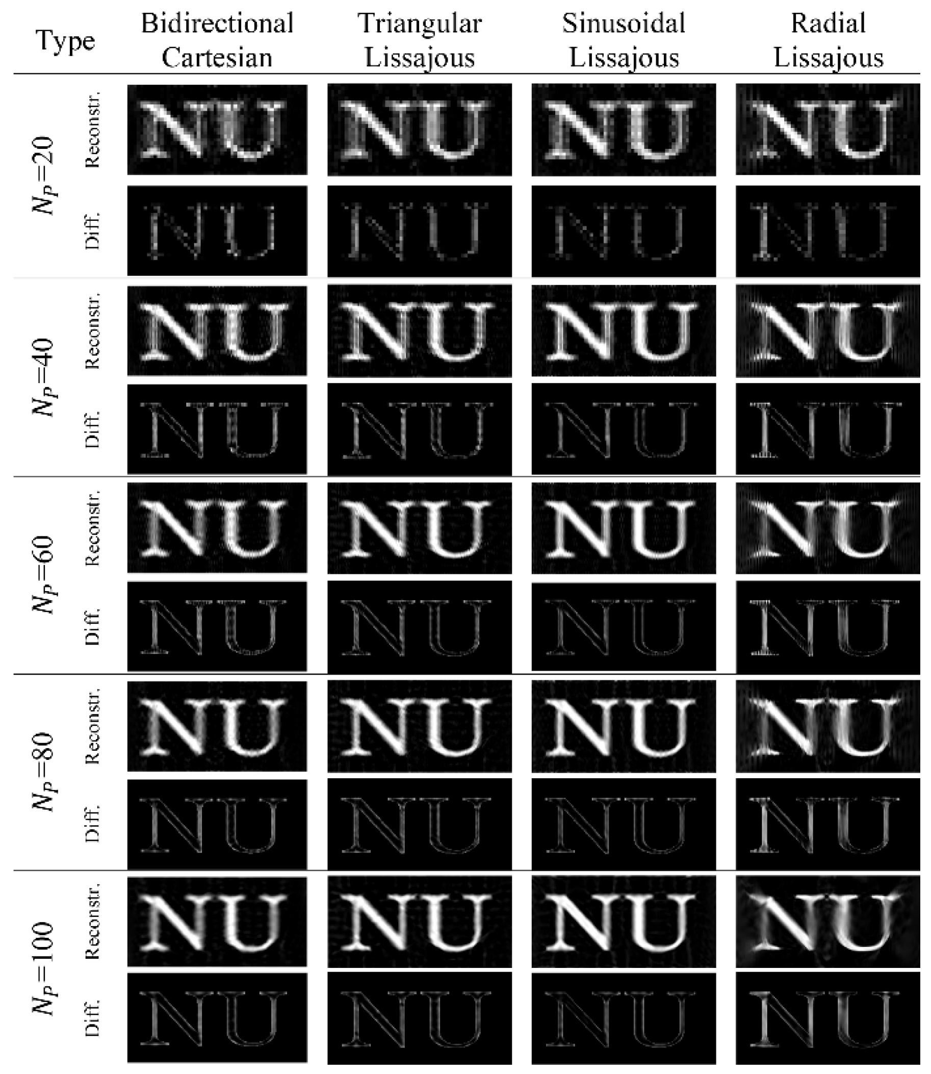
Figure A4.
Numerically generated values of reconstructed image using sinusoidal Lissajous mesh for (a) PSNR, (b) SSIM, (c) RMSE, and (d) NTE over varying for various scanning trajectories.
Figure A4.
Numerically generated values of reconstructed image using sinusoidal Lissajous mesh for (a) PSNR, (b) SSIM, (c) RMSE, and (d) NTE over varying for various scanning trajectories.

References
- Bauweraerts, P.; Meyers, J. Reconstruction of turbulent flow fields from lidar measurements using large-eddy simulation. J. Fluid Mech. 2021, 906, A17. [Google Scholar] [CrossRef]
- Wu, J.-W.; Lin, Y.-T.; Lo, Y.-T.; Liu, W.-C.; Fu, L.-C. Lissajous Hierarchical Local Scanning to Increase the Speed of Atomic Force Microscopy. IEEE Trans. Nanotechnol. 2015, 14, 810–819. [Google Scholar] [CrossRef]
- Vinke, E.J.; de Groot, M.; Venkatraghavan, V.; Klein, S.; Niessen, W.J.; Ikram, M.A.; Vernooij, M.W. Trajectories of imaging markers in brain aging: The Rotterdam Study. Neurobiol. Aging 2018, 71, 32–40. [Google Scholar] [CrossRef] [PubMed]
- Kasban, H.; El-Bendary, M.A.M.; Salama, D.H. A Comparative Study of Medical Imaging Techniques. Int. J. Inf. Sci. Intell. Syst. 2015, 4, 37–58. [Google Scholar]
- Weiss, T.; Senouf, O.; Vedula, S.; Michailovich, O.; Zibulevsky, M.; Bronstein, A. PILOT: Physics-Informed Learned Optimized Trajectories for Accelerated MRI. J. Mach. Learn. Biomed. Imaging 2019, 6, 1–23. [Google Scholar] [CrossRef]
- Bogner, W.; Otazo, R.; Henning, A. Accelerated MR spectroscopic imaging—A review of current and emerging techniques. NMR Biomed. 2021, 34, 1–32. [Google Scholar] [CrossRef] [PubMed]
- Werner, F.; Gdaniec, N.; Knopp, T. First experimental comparison between the Cartesian and the Lissajous trajectory for magnetic particle imaging. Phys. Med. Biol. 2017, 62, 3407–3421. [Google Scholar] [CrossRef]
- Knopp, T.; Biederer, S.; Sattel, T.; Weizenecker, J.; Gleich, B.; Borgert, J.; Buzug, T.M. Trajectory analysis for magnetic particle imaging. Phys. Med. Biol. 2009, 54, 385–397. [Google Scholar] [CrossRef]
- Le, T.-A.; Bui, M.P.; Yoon, J. Development of Small-Rabbit-Scale Three-Dimensional Magnetic Particle Imaging System With Amplitude-Modulation-Based Reconstruction. IEEE Trans. Ind. Electron. 2023, 70, 3167–3177. [Google Scholar] [CrossRef]
- Le, T.A.; Bui, M.P.; Yoon, J. Optimal Design and Implementation of a Novel Two-Dimensional Electromagnetic Navigation System That Allows Focused Heating of Magnetic Nanoparticles. IEEE/ASME Trans. Mechatron. 2021, 26, 551–562. [Google Scholar] [CrossRef]
- Mukhatov, A.; Le, T.-A.; Pham, T.T.; Do, T.D. A comprehensive review on magnetic imaging techniques for biomedical applications. Nano Select 2023, 4, 213–230. [Google Scholar] [CrossRef]
- Borcs, A.; Benedek, C. Extraction of Vehicle Groups in Airborne Lidar Point Clouds With Two-Level Point Processes. Geosci. Remote Sens. IEEE Trans. 2015, 53, 1475–1489. [Google Scholar] [CrossRef]
- Leoncini, M.; Bestetti, M.; Bonfanti, A.; Facchinetti, S.; Minotti, P.; Langfelder, G. Fully Integrated, 406 μA, 5/hr, Full Digital Output Lissajous Frequency-Modulated Gyroscope. IEEE Trans. Ind. Electron. 2019, 66, 7386–7396. [Google Scholar] [CrossRef]
- Weiss, U.; Biber, P. Plant detection and mapping for agricultural robots using a 3D LIDAR sensor. Rob. Auton. Syst. 2011, 59, 265–273. [Google Scholar] [CrossRef]
- Fink, M.; Schardt, M.; Baier, V.; Wang, K.; Jakobi, M.; Koch, A.W. Low-cost scanning LIDAR architecture with a scalable frame rate for autonomous vehicles. Appl. Opt. 2023, 62, 675–682. [Google Scholar] [CrossRef]
- Karimi, M.; Oelsch, M.; Stengel, O.; Babaians, E.; Steinbach, E. LoLa-SLAM: Low-Latency LiDAR SLAM Using Continuous Scan Slicing. IEEE Robot. Autom. Lett. 2021, 6, 2248–2255. [Google Scholar] [CrossRef]
- Wang, J.; Zhang, G.; You, Z. Improved sampling scheme for LiDAR in Lissajous scanning mode. Microsyst. Nanoeng. 2022, 8, 64. [Google Scholar] [CrossRef] [PubMed]
- Bazaei, A.; Yong, Y.K.; Moheimani, S.O.R. High-speed Lissajous-scan atomic force microscopy: Scan pattern planning and control design issues. Rev. Sci. Instrum. 2012, 83, 1–10. [Google Scholar] [CrossRef]
- Top, C.B.; Güngör, A. Tomographic Field Free Line Magnetic Particle Imaging with an Open-Sided Scanner Configuration. IEEE Trans. Med. Imaging 2020, 39, 4164–4173. [Google Scholar] [CrossRef]
- von Haxthausen, F.; Böttger, S.; Wulff, D.; Hagenah, J.; García-Vázquez, V.; Ipsen, S. Medical Robotics for Ultrasound Imaging: Current Systems and Future Trends. Curr. Robot. Rep. 2021, 2, 55–71. [Google Scholar] [CrossRef]
- Reinhardt, S.C.M.; Masullo, L.A.; Baudrexel, I.; Steen, P.R.; Kowalewski, R.; Eklund, A.S.; Strauss, S.; Unterauer, E.M.; Schlichthaerle, T.; Strauss, M.T.; et al. Ångström-resolution fluorescence microscopy. Nature 2023, 617, 711–716. [Google Scholar] [CrossRef]
- Vogel, P.; Kampf, T.; Herz, S.; Ruckert, M.A.; Bley, T.A.; Behr, V.C. Adjustable Hardware Lens for Traveling Wave Magnetic Particle Imaging. IEEE Trans. Magn. 2020, 56, 1–6. [Google Scholar] [CrossRef]
- Top, C.B.; Güngör, A.; Ilbey, S.; Güven, H.E. Trajectory analysis for field free line magnetic particle imaging. Med. Phys. 2019, 46, 1592–1607. [Google Scholar] [CrossRef] [PubMed]
- Ozaslan, A.A.; Alacaoglu, A.; Demirel, O.B.; Cukur, T.; Saritas, E.U. Fully automated gridding reconstruction for non-Cartesian x-space magnetic particle imaging. Phys. Med. Biol. 2019, 64, 165018. [Google Scholar] [CrossRef] [PubMed]
- Tanguy, Q.A.A.; Gaiffe, O.; Passilly, N.; Cote, J.-M.; Cabodevila, G.; Bargiel, S.; Lutz, P.; Xie, H.; Gorecki, C. Real-time Lissajous imaging with a low-voltage 2-axis MEMS scanner based on electrothermal actuation. Opt. Express 2020, 28, 8512. [Google Scholar] [CrossRef] [PubMed]
- Wang, J.; Zhang, G.; You, Z. Design rules for dense and rapid Lissajous scanning. Microsyst. Nanoeng. 2020, 6, 4–10. [Google Scholar] [CrossRef] [PubMed]
- Bakenecker, A.C.; Ahlborg, M.; Debbeler, C.; Kaethner, C.; Buzug, T.M.; Lüdtke-Buzug, K. Magnetic particle imaging in vascular medicine. Innov. Surg. Sci. 2020, 3, 179–192. [Google Scholar] [CrossRef] [PubMed]
- Boiroux, D.; Oke, Y.; Miwakeichi, F.; Oku, Y. Pixel timing correction in time-lapsed calcium imaging using point scanning microscopy. J. Neurosci. Methods 2014, 237, 60–68. [Google Scholar] [CrossRef] [PubMed]
- Knopp, T.; Buzug, T.M. Magnetic Particle Imaging: An Introduction to Imaging Principles and Scanner Instrumentation; Springer: Berlin/Heidelberg, Germany, 2012; pp. 54–57. ISBN 9783642041990. [Google Scholar]
- Tuma, T.; Lygeros, J.; Kartik, V.; Sebastian, A.; Pantazi, A. High-speed multiresolution scanning probe microscopy based on Lissajous scan trajectories. Nanotechnology 2012, 23, 185501. [Google Scholar] [CrossRef]
- Biederer, S. Magnet-Partikel-Spektrometer: Entwicklung Eines Spektrometers zur Analyse Superparamagnetischer Eisenoxid-Nanopartikel für Magnetic-Particle-Imaging; Springer: Berlin/Heidelberg, Germany, 2012; pp. 14–17. ISBN 3834824070. [Google Scholar]
- Zhang, P.; Liu, J.; Li, Y.; Yin, L.; An, Y.; Zhong, J.; Hui, H.; Tian, J. Dual-Feature Frequency Component Compression Method for Accelerating Reconstruction in Magnetic Particle Imaging. IEEE Trans. Comput. Imaging 2023, 9, 289–297. [Google Scholar] [CrossRef]
- Abdullah-Al-Mamun, M.; Tyagi, V.; Zhao, H. A New Full-Reference Image Quality Metric for Motion Blur Profile Characterization. IEEE Access 2021, 9, 156361–156371. [Google Scholar] [CrossRef]
- Muckley, M.J.; Riemenschneider, B.; Radmanesh, A.; Kim, S.; Jeong, G.; Ko, J.; Jun, Y.; Shin, H.; Hwang, D.; Mostapha, M.; et al. Results of the 2020 fastMRI Challenge for Machine Learning MR Image Reconstruction. IEEE Trans. Med. Imaging 2021, 40, 2306–2317. [Google Scholar] [CrossRef] [PubMed]
- Ahmadian, K.; Reza-Alikhani, H.-R. Self-Organized Maps and High-Frequency Image Detail for MRI Image Enhancement. IEEE Access 2021, 9, 145662–145682. [Google Scholar] [CrossRef]
- Duan, J.; Liu, C.; Liu, Y.; Shang, Z. Adaptive Transform Learning and Joint Sparsity Based PLORAKS Parallel Magnetic Resonance Image Reconstruction. IEEE Access 2020, 8, 212315–212326. [Google Scholar] [CrossRef]
- Wang, J.; Qiao, L.; Lv, H.; Lv, Z. Deep Transfer Learning-Based Multi-Modal Digital Twins for Enhancement and Diagnostic Analysis of Brain MRI Image. IEEE/ACM Trans. Comput. Biol. Bioinform. 2023, 20, 2407–2419. [Google Scholar] [CrossRef] [PubMed]
- Huang, Y.; Preuhs, A.; Manhart, M.; Lauritsch, G.; Maier, A. Data Extrapolation From Learned Prior Images for Truncation Correction in Computed Tomography. IEEE Trans. Med. Imaging 2021, 40, 3042–3053. [Google Scholar] [CrossRef] [PubMed]
- Wang, Z.; Sun, Y.; Liao, J.; Cao, R.; Wang, C.; Jin, L.; Feng, J.; Cao, C. Image Reconstruction of Targets Undergoing Complex Motion Based on Optical Phased Array Compressed-Sensing Ghost Imaging Technology. J. Light. Technol. 2022, 40, 7746–7756. [Google Scholar] [CrossRef]
- Mukaddim, R.A.; Meshram, N.H.; Weichmann, A.M.; Mitchell, C.C.; Varghese, T. Spatiotemporal Bayesian Regularization for Cardiac Strain Imaging: Simulation and In Vivo Results. IEEE Open J. Ultrason. Ferroelectr. Freq. Control 2021, 1, 21–36. [Google Scholar] [CrossRef]
Figure 1.
Scanning trajectories with nearest (red dashed lines)/furthest (green dashed lines) nearest neighbor points and maximum perpendicular distance for = 12. (a) Bidirectional Cartesian. (b) Triangular Lissajous. (c) Sinusoidal Lissajous. (d) Radial Lissajous.
Figure 1.
Scanning trajectories with nearest (red dashed lines)/furthest (green dashed lines) nearest neighbor points and maximum perpendicular distance for = 12. (a) Bidirectional Cartesian. (b) Triangular Lissajous. (c) Sinusoidal Lissajous. (d) Radial Lissajous.

Figure 2.
Theoretical and numerically calculated values of (a) and (b) for sinusoidal Lissajous over various values.
Figure 2.
Theoretical and numerically calculated values of (a) and (b) for sinusoidal Lissajous over various values.
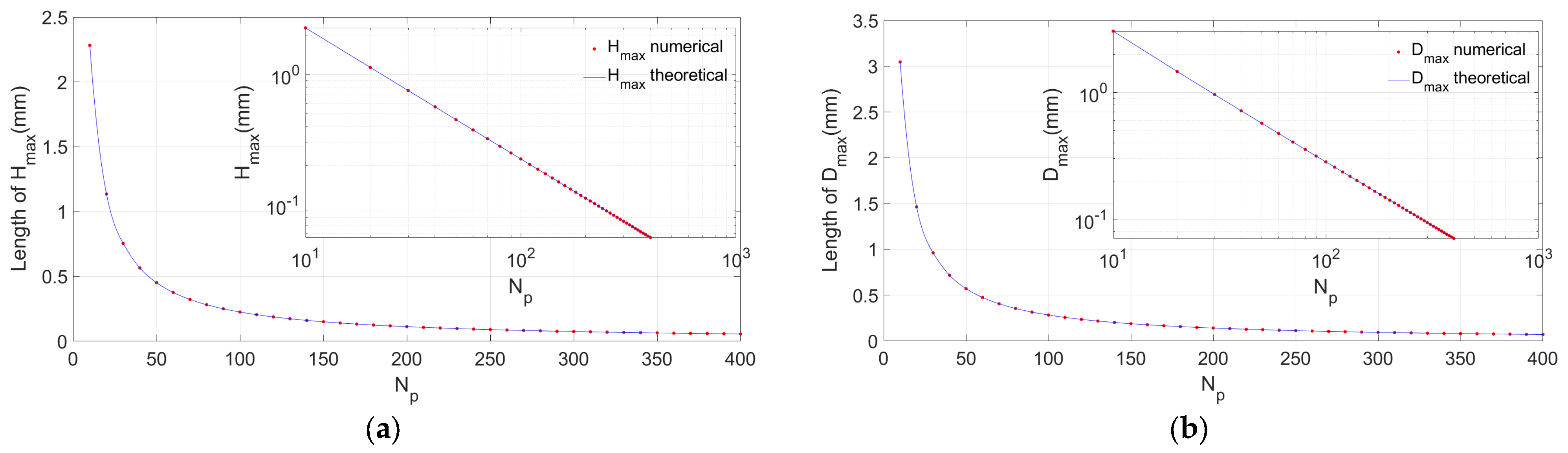
Figure 3.
The maximum values for , , and over a range of values were calculated numerically, along with the corresponding fitted curves for the following trajectories: (a) bidirectional Cartesian, (b) triangular Lissajous, (c) sinusoidal Lissajous, (d) radial Lissajous. Plots of the values for each trajectory are shown in (e).
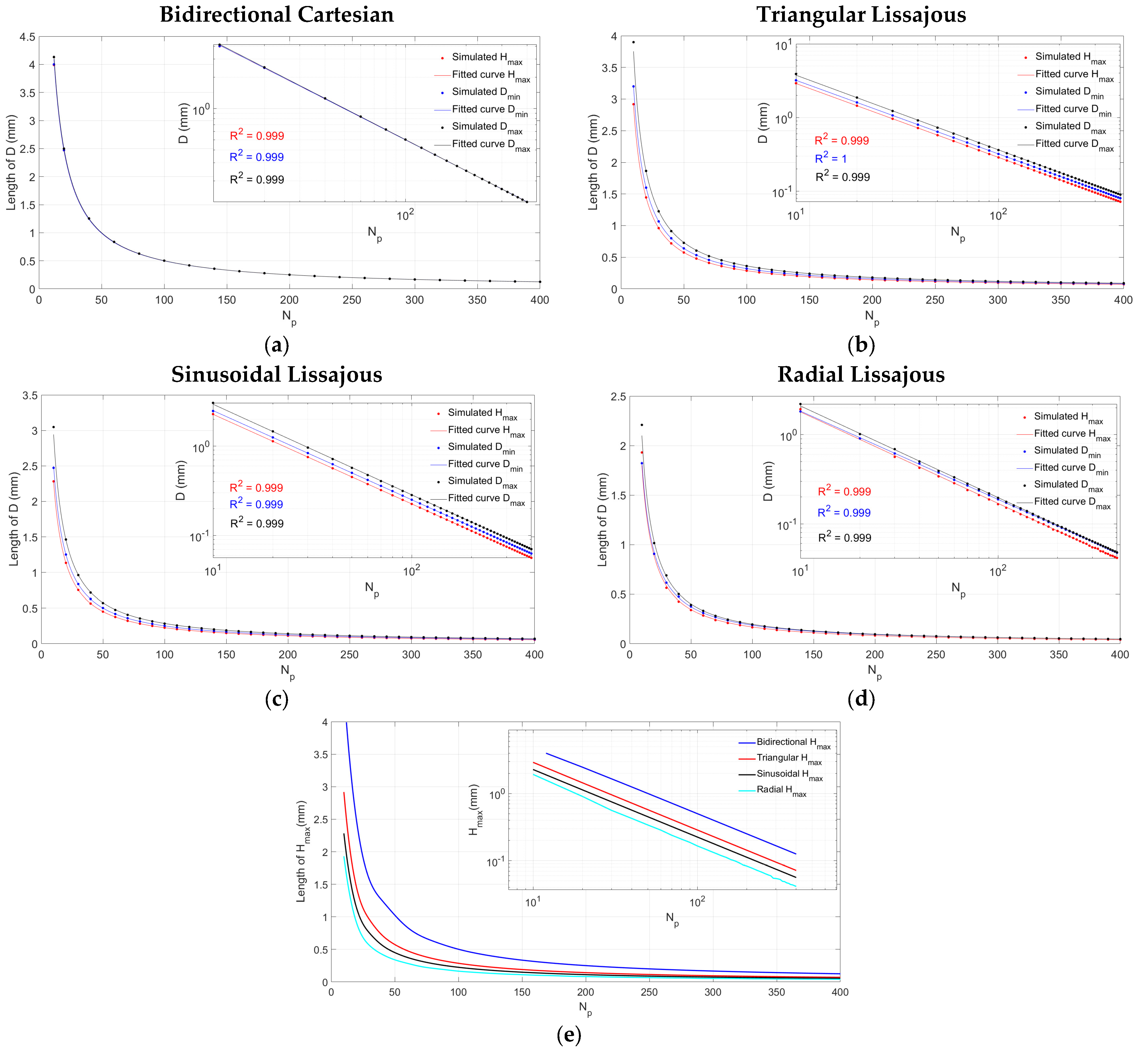
Figure 4.
Fill factor as a function of values for all scanning trajectories using (a) bidirectional Cartesian pixel size, (b) triangular Lissajous pixel size, (c) sinusoidal Lissajous pixel size, and (d) radial Lissajous pixel size.
Figure 4.
Fill factor as a function of values for all scanning trajectories using (a) bidirectional Cartesian pixel size, (b) triangular Lissajous pixel size, (c) sinusoidal Lissajous pixel size, and (d) radial Lissajous pixel size.
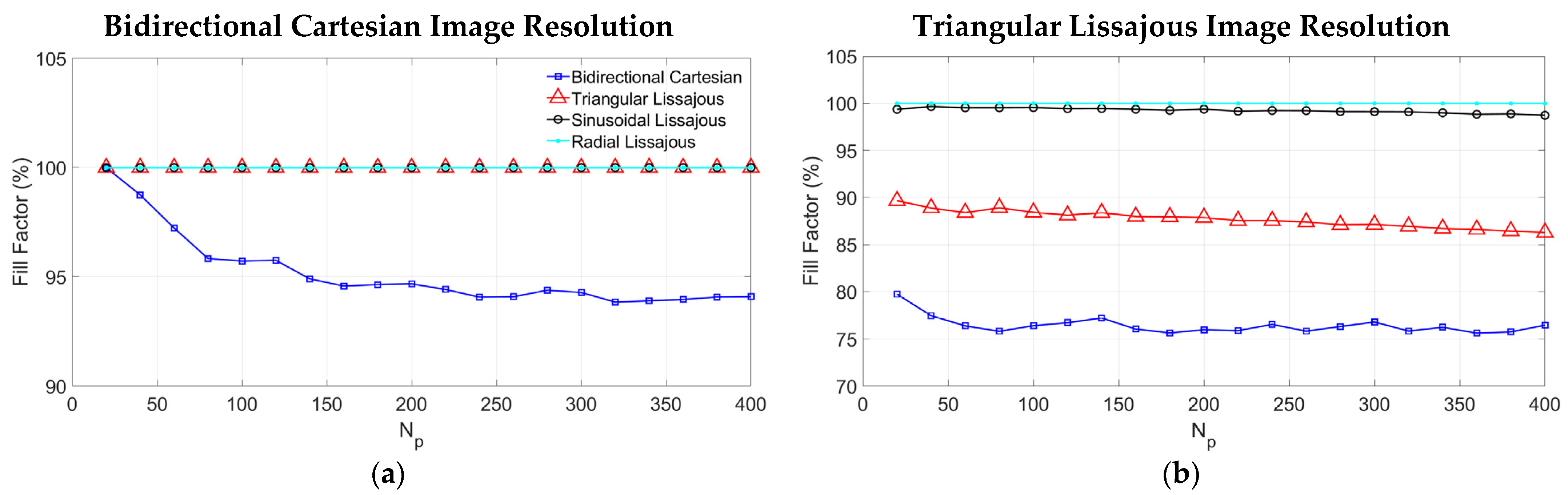

Figure 5.
(a) Phantom image used for the reconstruction and (b) the outcomes of the reconstructed images using bidirectional Cartesian mesh (i.e., 0.5 value of BC was used as the pixel size) for various scanning patterns and .
Figure 5.
(a) Phantom image used for the reconstruction and (b) the outcomes of the reconstructed images using bidirectional Cartesian mesh (i.e., 0.5 value of BC was used as the pixel size) for various scanning patterns and .
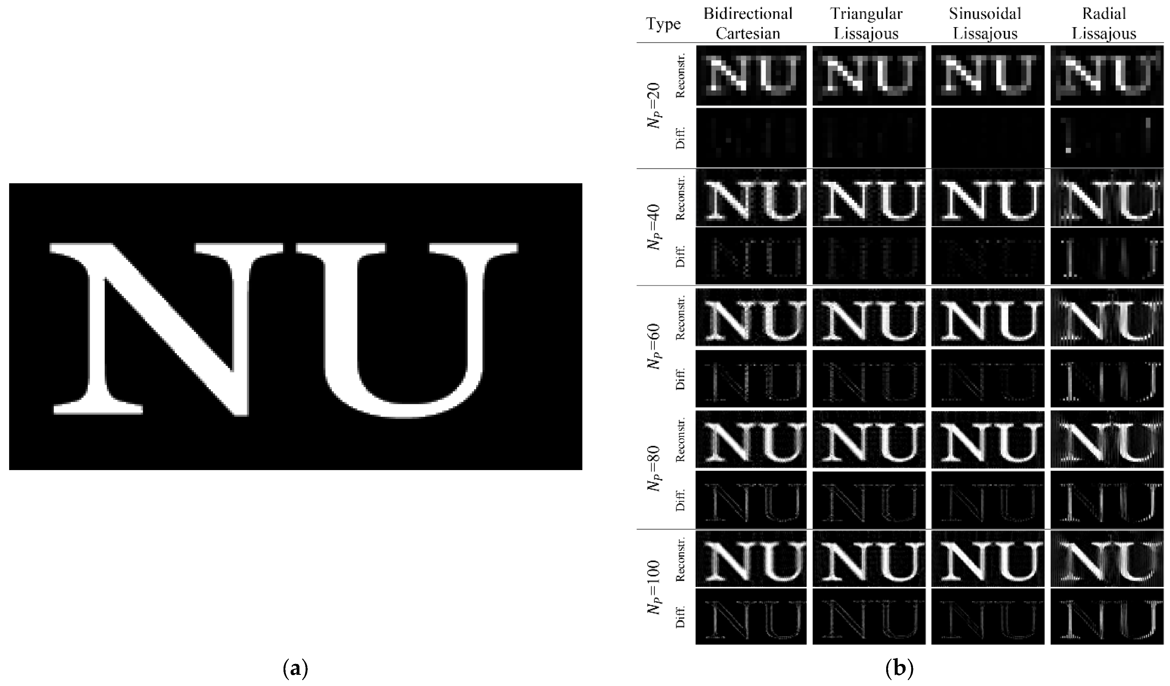
Figure 6.
Numerically generated values of reconstructed image using bidirectional Cartesian mesh for (a) PSNR, (b) SSIM, (c) RMSE, and (d) NTE over varying for various scanning trajectories.
Figure 6.
Numerically generated values of reconstructed image using bidirectional Cartesian mesh for (a) PSNR, (b) SSIM, (c) RMSE, and (d) NTE over varying for various scanning trajectories.

Table 1.
Mathematical expressions for all scanning trajectories used in this work [24].
Table 1.
Mathematical expressions for all scanning trajectories used in this work [24].
| Trajectories | Mathematical Expression | Frequency Ratio and Repetition Time | Advantages | Disadvantages | |
|---|---|---|---|---|---|
| Bidirectional Cartesian [24] | (3) |
|
| ||
| (4) | |||||
| Triangular Lissajous [8] | (5) |
|
| ||
| (6) | |||||
| Sinusoidal Lissajous [8] | (7) |
|
| ||
| (8) | |||||
| Radial Lissajous [24] | (9) |
|
| ||
| (10) | |||||
Table 2.
Maximum distance to nearest neighboring points in mm for different trajectories using the proposed method with = 100.
Table 2.
Maximum distance to nearest neighboring points in mm for different trajectories using the proposed method with = 100.
| B.C. | 0.502 | 0.502 | 0.503 |
| T.L. | 0.287 | 0.320 | 0.361 |
| S.L. | 0.225 | 0.251 | 0.283 |
| R.L. | 0.166 | 0.188 | 0.195 |
Table 3.
Constant and values resulting from a hyperbola fit, as shown in (11).
| B.C. | T.L. | S.L. | R.L. | ||
|---|---|---|---|---|---|
| Max | 0.991 | 1.003 | 1.003 | 1.026 | |
| 0.021 | 0.034 | 0.044 | 0.052 | ||
| Max | 0.992 | 1.000 | 0.998 | 0.991 | |
| 0.021 | 0.031 | 0.040 | 0.056 | ||
| Max | 0.997 | 1.014 | 1.014 | 1.028 | |
| 0.020 | 0.026 | 0.033 | 0.045 |
Table 4.
Constant and their values resulting from a hyperbola fit when , as shown in (12).
| B.C. | T.L. | S.L. | R.L. | ||
|---|---|---|---|---|---|
| Max | 0.022 | 0.034 | 0.043 | 0.046 | |
| 0.999 | 0.999 | 0.999 | 0.999 | ||
| Max | 0.022 | 0.031 | 0.040 | 0.058 | |
| 0.999 | 1.000 | 0.999 | 0.999 | ||
| Max | 0.020 | 0.024 | 0.031 | 0.040 | |
| 0.999 | 0.999 | 0.999 | 0.998 |
Table 5.
Parameters used for reconstruction of image.
| Pixel Size | 0.5 of BC mesh |
| Values | 20, 40, 60, 80, 100 |
| Particle Diameter | 30 × 10−9 m |
| Temperature | 310 K |
| Permeability of Air | 4π × 10−7 N/A2 |
| Concentration of Particles | 1.5 mol/m3 |
| Molar Mass of SPION | 0.231 kg/mol |
| Density of SPION | 5170 kg/m3 |
Disclaimer/Publisher’s Note: The statements, opinions and data contained in all publications are solely those of the individual author(s) and contributor(s) and not of MDPI and/or the editor(s). MDPI and/or the editor(s) disclaim responsibility for any injury to people or property resulting from any ideas, methods, instructions or products referred to in the content. |
© 2023 by the authors. Licensee MDPI, Basel, Switzerland. This article is an open access article distributed under the terms and conditions of the Creative Commons Attribution (CC BY) license (https://creativecommons.org/licenses/by/4.0/).
Share and Cite
MDPI and ACS Style
Mukhatov, A.; Le, T.-A.; Do, T.D.; Pham, T.T. Universal Behavior of the Image Resolution for Different Scanning Trajectories. Appl. Syst. Innov. 2023, 6, 103. https://doi.org/10.3390/asi6060103
AMA Style
Mukhatov A, Le T-A, Do TD, Pham TT. Universal Behavior of the Image Resolution for Different Scanning Trajectories. Applied System Innovation. 2023; 6(6):103. https://doi.org/10.3390/asi6060103
Chicago/Turabian StyleMukhatov, Azamat, Tuan-Anh Le, Ton Duc Do, and Tri T. Pham. 2023. "Universal Behavior of the Image Resolution for Different Scanning Trajectories" Applied System Innovation 6, no. 6: 103. https://doi.org/10.3390/asi6060103