Design and Development of Complex-Order PI-PD Controllers: Case Studies on Pressure and Flow Process Control

Abstract

This article examines the performance of the proposed complex-order, conventional and fractional-order controllers for process automation and control in process plants. The controllers are compared regarding disturbance rejection and set-point tracking, considering variables such as response time, robustness to uncertainty, and steady-state error. The study shows that a complex PI-PD controller has better accuracy, faster response time, and better noise rejection. Still, implementation is challenging due to increased complexity and processing requirements. In contrast, a standard PI-PD controller is a known solution but may have problems with accuracy and robustness. Fractional-order controllers based on fractional computations have the potential to improve control accuracy and robustness of non-linear and time-varying systems. Experimental insights and real-world case studies are used to highlight the strengths and weaknesses of each controller. The findings provide valuable insights into the strengths and weaknesses of complex-order and fractional-order controllers and help to select the appropriate controller for specific process plant requirements. Future perspectives on controller design and performance optimization are detailed, identifying the potential benefits of using complex and fractional-order controllers in process plants.

1. Introduction

Pressure and level process plants are widely utilized in various industrial applications, including chemical, petrochemical, and food processing [1,2]. Process plants commonly experience dynamic set point changes and disturbances significantly affecting control performance [3]. Commonly, PID (proportional–integral–derivative) controllers are used to control these processes in an efficient operation of these factories, which is critical to maintaining product quality and reducing operating costs. Traditional PID controllers sometimes respond promptly and effectively, resulting in slow response times, overshoots, and poor noise rejection [4]. Further, systems that exhibit non-minimal phase responses, high-order dynamics, and extensive transmission delays often limit the PID controllers’ performance [5]. The complex-order controller is a fractional order designed to overcome the limitations of regular PID controllers. Complex-order PI (proportional–integral)-PD (proportional–derivative) controllers have fractional derivative and integral terms, allowing the controller to operate with high dynamics and longer transit delays [6].

A PID controller is a standard feedback control system seen in industrial environments, which is essential for the controlling system output depending on the input. The system performance varies with a proportional component proportional to the deviation between target performance and actual performance [5]. The integral component continuously corrects for steady-state errors by integrating accumulated errors over time. Abrupt fluctuations in the error rate are predicted and compensated for by the derivative component. PID controllers are widely used in most industries, such as temperature control, motor speed control, pump flow control, satellite communications [7], and aircraft altitude control [8]. Recently, PID has been used in robotics, robotic systems, and computer numerical control systems due to its advantages, including simple tuning, maintaining system stability, and minimizing overshoot [9]. It offers greater accuracy than manual adjustment methods and the flexibility to adjust the system output to various operating conditions [10]. PID controllers can be implemented in digital or analogue systems. Still, digital PID controllers are generally more accurate and more accessible to implement, quickly responding to input changes and adjusting system outputs accordingly [11].

In the literature, an algorithmic optimization technique based on the flower pollination algorithm [12] tunes a PI-PD cascade controller. It evaluated its performance based on settling time, overshoot, and undershoot. Similarly, researchers in [13] achieved the settling time, overshoot, and phase margin using their cascaded fractional-order PI-PD approach for the inverted pendulum. In [14], the researchers used arithmetic and trigonometric operators to obtain the fractional-order predictive PI controller parameters using the integer absolute time error (ITAE) as the objective function to achieve effective set-point tracking and disturbance rejection performance. In another study, hybrid probabilistic fractal search and pattern search techniques were used to tune a cascaded PI-PD controller and evaluated its performance based on the settling time, integer squared error (ISE), integer time squared error (ITSE), integer absolute error (IAE), and ITAE [15].

In [16], Shanthini et al. used particle swarm optimization (PSO) and genetic algorithms to tune PID, I-PD, and fractional order PI-PD controllers in a DC-DC converter, where the performance criteria are the settling time and overshoot. In addition, modified PI-PD controllers are tuned using an automated tuning method, and their performance has been assessed based on the settling time, overshoot, and IAE, with comparisons made against conventional PID and modified PID controllers [17]. The Ziegler–Nichols tuning method to design PI-PD controllers and performance has been evaluated based on the settling time, overshoot, and integral absolute error (IAE) [18]. Several studies were conducted using vector tuning, and trial-and-error approaches tuned fractional-order PI-PD controllers for a DC motor in the frequency frame and assessed performance based on steady-state errors [19].

Roong et al., in [20], used the PSO algorithm to tune a fractional-order PI-PD controller for position control in a magnetic levitation system, evaluating overshooting and settling time performance. In another study [21], the Ziegler–Nichols method is used to design a PI-PD controller for voltage regulation of building-integrated photovoltaic and wind turbine systems, with the performance based on voltage. Similarly, in [22], the authors used the Ziegler–Nichols method to tune their PI-PD and I-PD controllers for speed control of DC motors and evaluated their performance based on the ISE and settling time. The study conducted in [23] used the Ziegler–Nichols method to tune a PI-PD controller for unstable control systems using sampled data and compared its performance in terms of ISE, overshoot, and settling time with that of the PID controller.

Recent studies emphasize the importance of a rigorous performance assessment to evaluate the efficacy of PI-PD controllers due to their potential for better performance and stability. Researchers used specific performance measures tailored to the system’s characteristics to quantify the PI-PD controller’s performance and compare it with other controller types [1,2,12,24]. Some performance measures used in the reviewed studies include settling time, overshoot, rise time, peak time, load disturbance, absolute error, phase and gain margins, ISE, ITSE, IAE, ITAE, and time response. These measurements evaluated different aspects of controller performance, including stability, speed of response, accuracy, ability to reject interference, and robustness. The choice of tuning method has been crucial in optimizing the PI-PD controller’s performance. The results of the reviewed studies highlighting the versatility of PI-PD controllers in controlling different types of systems and processes are summarized and given in

Table 1. Summary of the works related to complex-order PID controllers.

Ref.	Controller	Tuning Technique	No. of Parameters	System	Comparing Controllers	Performance Measure
[2]	PI-PD	Auto tuning	4	First and second-order unstable system with time delay	PID	Peak time, IAE, Settling time, Overshoot, Rise time
[12]	PI-PD	Ziegler–Nichols	4	First-order plus dead time (stable and unstable system)	I, PI, and PID	Settling time, Peak overshoot, Peak undershoot (-ve), IAE, ISE, ITAE, ITSE
[24]	PI-PD	Particle Swarm Optimization (PSO)	4	Antilock braking system	Feedback linearization	Friction coefficient ($\mu$), Settling time, Rise time, Stopping distance (m), Range of torque (N.m)
[25]	PI-PD	Trial and error	4	First and second-order system, higher-order unstable dead time system	PI and PID	Steady state error, Settling time, Peak overshoot
[26]	PI-PD	Ziegler–Nichols	4	Second-order system, temperature control for oil-cooling machines	PID and modified PID	Disturbance rejection
[20]	PI-PD	Trial and error	4	Magnetic levitation system	Feedforward PI-PD	Settling time, Overshoot
[21]	PI-PD	Trial and error	4	Photovoltaic and wind turbine system	IPI, FOPI	Voltage
[27]	PI-PD	Polynomial curve fitting techniques	4	First and second-order system with time delay	PID	Settling time, Overshoot, Jmin
[28]	Fractional-order PI-PD	Ziegler–Nichols	6	Pressure process	PID, FOPID, PI-PD, and FOPI-PD	Rise time, Settling time, IAE Peak overshoot, ISE
[29]	Fractional-order PI-PD	Trial and error	5	Second-order dead time and oscillatory system	PI-PD	Rise time, IAE, Settling time, Peak overshoot
[16]	Fractional-order PI-PD	PSO and Genetic algorithm	4	DC-DC converter	PID, I-PD, and FOPI-PD	Settling time, Overshoot
[30]	Fractional-order PI-PD	Bode’s integrals	6	pH control, distillation column and liquid level plant	FOPI and FOPD	Overshoot, settling time and ITAE
[31]	Fractional-order PI-PD	Stability boundary locus and the weighted geometrical centre	6	pH control and multiple dead time process models	Different PI-PD control designs	Statistical analysis
[15]	Cascade PI-PD	Stochastic fractal search and Pattern search algorithm	4	Plug-in Electric Vehicles	PI and PID	Settling time, IAE, ISE, ITAE, ITSE
[13]	Fractional-order cascaded PI-PD	Graphical method	6	Cart-Inverted Pendulum, second and third-order linear time-invariant unstable system	PI λ-PDμ, ${\left[PI\right]}^{\lambda }$-${\left[PD\right]}^{\mu }$, PIλDμ	Settling time, Overshoot, Phase margin (deg), Bandwidth (rad/s), Delay margin (${\tau }_d$)
[17]	Modified PI-PD	Auto tuning	7	DC motor, automatic voltage regulator	PID, modified PID, and modified PI-PD	Settling time, Overshoot, IAE
[18]	Modified PI-PD	Ziegler–Nichols	7	Aircraft pitch angle and disc position control	PID	Settling time, Overshoot, IAE, Gain and Phase margin
[32]	Improved PI-PD	Trial and error	6	FOPTD DC motor model	-	Steady state error
[21]	Modified PI-PD Smith predictor	Auto tuning	4	Multiple dead time process models	Smith predictor PI and Smith predictor PID	Settling time, Overshoot
[22]	Optimal PI-PD	Cuckoo search algorithm	4	DC motor, third-order system transfer function	I-PD	Settling time, ISE

.

The reviewed studies demonstrated different tuning methods to determine appropriate controller parameters, including automatic optimization [2], the Ziegler–Nichols method [5,12,33], and PSO algorithms [24,31,34]. Automated optimization techniques aim to simplify the controller design process for practitioners by automating the parameter tuning process. On the other hand, the Ziegler–Nichols method and the PSO algorithm are more sophisticated approaches that allow fine-tuning of the controller parameters to achieve desired performance characteristics.

The studies demonstrated the effectiveness of complex PID and PI-PD controllers in controlling unstable processes with dead time [2], stable and unstable processes with first order plus dead time [12], higher-order dead-time systems [31,35], anti-lock braking systems [24], real-time pressure used in processes [14], oil chiller temperature control [26], and other applications [29,36,37]. PI-PD controllers showed better settling time, overshoot, load disturbance rejection, and response speed than PID controllers and conventional controllers. Although peer-reviewed studies have provided valuable insights, there is still room for further research in PI-PD controllers for additional performance measures that capture other important aspects of control system performance.

Overall, the reviewed studies demonstrated the effectiveness and versatility of PI-PD controllers in controlling a wide range of systems and processes. Through exhaustive performance evaluation and the use of proper tuning methods, these controllers have demonstrated improved performance in terms of settling time, overshoot, noise rejection, and speed of response.

The study aims to develop a complex-order controller that considers the complex dynamics, non-minimum phase behaviour, and long transport delays commonly observed in industrial processes. The results of this research will contribute to the advancement of control strategies and support the selection and implementation of effective control systems in industrial applications, thereby optimizing process plant operation and improving control performance. The research involves the following:

1.

Developing a mathematical model that captures the dynamic reaction of a process plant.

2.

Designing an appropriate complex-order PI-PD controller.

3.

Conducting simulations and experiments to compare its performance with conventional PID controllers.

Furthermore, the study assesses the advantages and disadvantages of the proposed complex-order PI-PD controllers in dealing with disturbances and set-point changes to enhance control accuracy, response time, disturbance rejection, and overall stability. Findings from these studies contribute to further developing control system design and optimization, enabling more efficient and effective control of complex processes. Future research activities will explore additional performance metrics based on these findings, compare them with other advanced controllers, and develop new tuning methods to improve the performance of PI-PD controllers in various applications.

2. Development of Proposed Controller

This section provides a detailed discussion of the development of complex and fractional-order controllers.

2.1. Integer and Fractional-Order PID Controllers

PID is a feedback control algorithm extensively used in automation and engineering systems. It adjusts the system performance by calculating the difference between the desired set point and the actual value of the variable’s process. The three parameters of PID are $K_p$, $K_i$, and $K_d$, which determine its behaviour, and its controller block diagram is shown in Figure 1. The schematic depiction shows the set point denoted by $R\left(s\right)$, the system’s output response by $Y\left(s\right)$, the error by $E\left(s\right)$, and the controller signal by $U\left(s\right)$. It is worth noting that all these representations are in the Laplace domain, represented by the variable “s". The proportional gain ($K_p$) influences the control action based on the current error. A higher $K_p$ value results in a more aggressive response, leading the system towards the desired set point more quickly. However, setting $K_p$ too high can cause overshoot and instability, making it crucial to choose an optimal value. The integral gain ($K_i$) is a crucial parameter in control systems that helps eliminate steady-state errors and correct long-term deviations between desired settings and actual performance. On the other hand, the derivative gain ($K_d$) is a parameter in control systems that considers the error signal’s rate of change. Combining these three terms enables a PID controller to achieve stability, responsiveness, and precision in controlling various systems. The control signal of the PID controller is given as follows,

$$U\left(s\right)=\left(K_p+\frac{K_i}{s}+K_{d}s\right)E\left(s\right).$$

(1)

Fractional-order PID (FOPID) controllers are advanced versions of traditional PID controllers that utilize fractional-order computations to improve the control performance of complex systems [38]. In contrast to standard PID controllers that have three parameters (proportional, integral, and derivative gains), FOPID controllers incorporate two additional parameters ($\lambda$ and $\mu$) to achieve a better control performance. The FOPID controller’s $\lambda$ parameter modulates the integral gain over time, representing a time-varying factor that can be adjusted based on system dynamics. This allows the controller to adjust the integral gain to meet changing system behaviour and control needs. The $\mu$ parameter of the FOPID controller scales the integral gain, fine-tuning the magnitude of the integral response to system characteristics and control goals. Adjusting $\mu$ accordingly, the FOPID controller can adapt the integral response to meet specific control requirements. The FOPID controller’s block diagram is shown in Figure 1. The control signal of the FOPID controller is given as follows:

$$U\left(s\right)=\left(K_p+\frac{K_i}{s^{\lambda }}+K_d{s}^{\mu }\right)E\left(s\right),0<\lambda ,\mu <1.$$

(2)

Achieving optimal control performance in FOPID controllers requires careful $K_p$, $K_i$, $K_d$, $\lambda$, and $\mu$ tuning to balance responsiveness, stability, and robustness. Various optimization, heuristic, or model-based approaches can be employed to obtain appropriate parameter values for a specific control application. Integrating $\lambda$ and $\mu$ parameters and the standard gain elevates FOPID controllers’ performance by enhancing control accuracy, noise rejection, and adaptability to nonlinear and time-varying dynamics. These controllers are becoming increasingly popular in fields such as process control, robotics, and power electronics, where precise and robust control is crucial for handling complex system behaviour.

2.2. PI-PD Controller

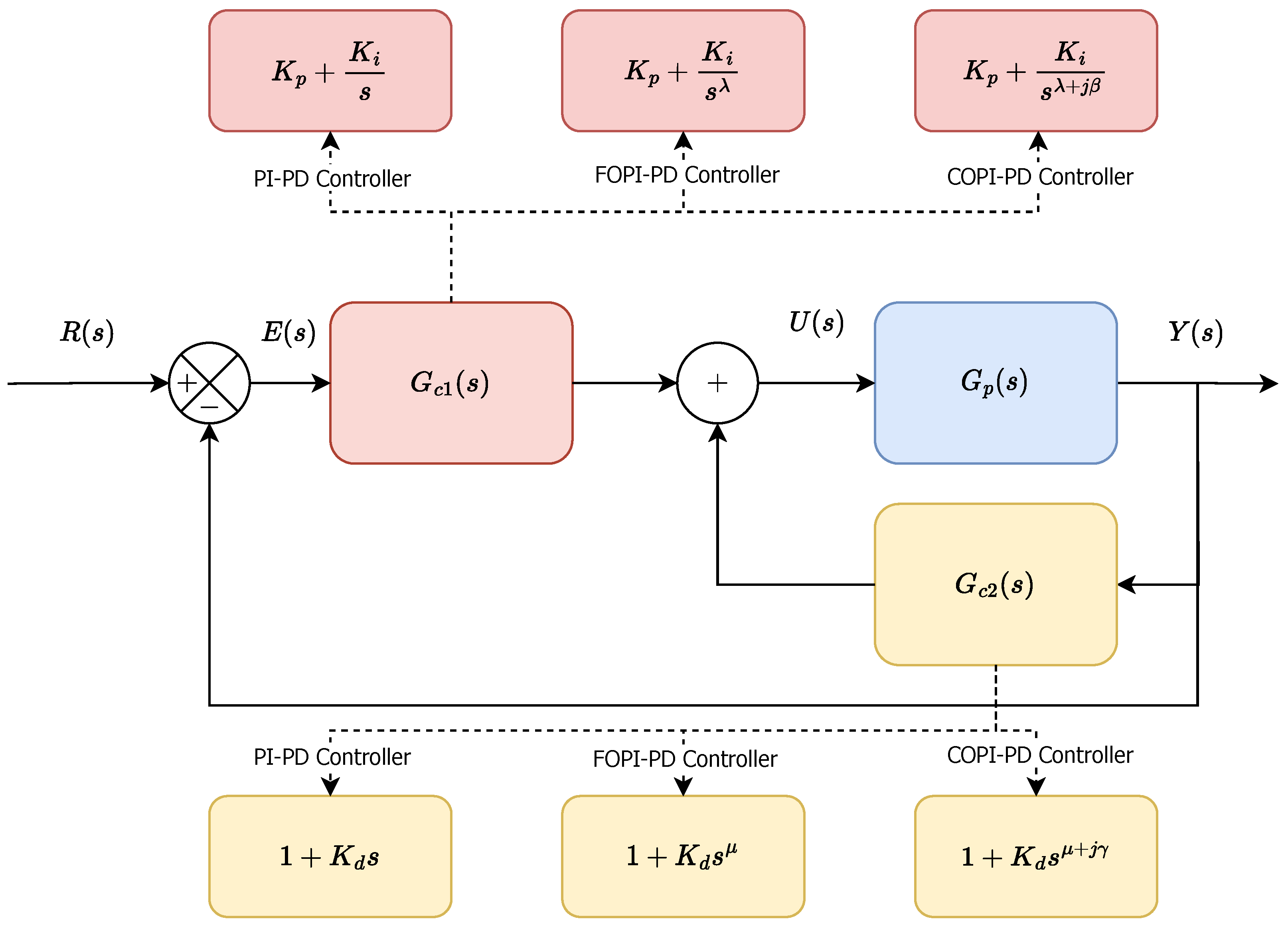
A PI-PD controller is a widely used feedback system in industrial settings. It merges proportional–integral (PI) and proportional–derivative (PD) control to regulate the system output by measuring the difference between the desired set point and the measured process variable, known as the error signal [5]. The PI parameters of the controller include two control processes: Proportional control (P) adjusts the output relative to the current error signal, providing an immediate corrective response. Integral control (I) integrates the error signal over time, adding corrective action to remove the steady-state error. It continually adjusts the output based on historically accumulated errors to ensure long-term accuracy and stability. The PI control components are highly effective at tracking set points and minimizing steady-state errors. They are an invaluable tool for industrial processes that require precision control and monitoring. The PI-PD controller’s block diagram is shown in Figure 2, and the control signal is given as follows:

$$U\left(s\right)=\left(K_p+\frac{K_i}{s}\right)E\left(s\right)+\left(1+K_{d}s\right)Y\left(s\right).$$

(3)

The PD parameter is a combination of proportional control and derivative control operations. The proportional control (P) responds to instantaneous error, while the derivative control (D) responds to the rate of change of error. This allows for a damping effect that reduces overshoot and improves the system response to error signal changes. By predicting future trends and adjusting the output accordingly, the PD controller component is instrumental in systems where a fast response to error signal changes is desired or damping is critical to prevent oscillations and instability. When the PI and PD parameters are combined, PI-PD controllers offer a balanced approach to control systems. PI parameters provide long-term accuracy and steady-state performance, while PD parameters improve transient response and damping characteristics. PI-PD controllers are widely used in various applications, such as process control, robotics, and motion control systems, as they provide flexible and robust control solutions.

2.3. Fractional-Order PI-PD Controller

Fractional-order PI-PD (FOPI-PD) controllers are advanced versions of traditional controllers that use fractional-order computation. These controllers employ $\lambda$ and $\mu$ parameters to enhance the control performance of systems with complex dynamics. The $\lambda$ parameter of a FOPI controller represents the fractional order of the integral action, which enables the controller to perform non-integer orders of integration to capture long-term memory effects and improve control performance. By adapting $\lambda$, the FOPID controller can adjust the integral action to the specific dynamics of the controlled system. Tuning $\lambda$ enables the FOPI controller to handle systems with non-linearity, time delays, and memory effects, depending on system complexity, desired control goal, and error signal characteristics. The FOPI-PD controller’s block diagram is shown in Figure 2. The control signal of the FOPI-PD controller is given as follows:

$$U\left(s\right)=\left(K_p+\frac{K_i}{s^{\lambda }}\right)E\left(s\right)+\left(1+K_d{s}^{\mu }\right)Y\left(s\right),0<\lambda ,\mu <1.$$

(4)

The $\mu$ parameter of the FOPD controller represents the fractional order of the derivative and controls the rate of change of the fractional-order error signal. The $\mu$-th order fractional derivative captures the system dynamics with memory effects and allows FOPD controllers to respond to complex behaviours not well captured by integer-th-order derivatives. The choice of $\mu$ depends on the dynamics and control requirements of the particular system. By adequately tuning $\mu$, FOPD controllers can effectively control systems with nonlinear and time-varying behaviour, improving control accuracy and stability. In the FOPI controller, the $\lambda$ introduces additional degrees of freedom and $\mu$ parameters, making it more flexible and adaptable than the traditional PI-PD controller. By customizing the fractional order of the integral and derivative actions, these controllers can better capture the complex system’s complex behaviour and improve control performance. Various tuning, optimization, or model-based approaches can be used to determine appropriate parameter values for a particular control application. Stability, responsiveness, and robust control gains should be tuned to the system’s specific characteristics to achieve the desired control performance.

2.4. Proposed Complex-Order PI-PD Controller

Complex-order PI-PD (COPI-PD) control is an advanced version of PID control that incorporates the principles of fractional and complex arithmetic. It employs complex orders $\lambda +j\beta$ in the integral and $\mu +j\gamma$ in the derivative terms to deliver more precise control responses, particularly in complex systems. The complex orders enables engineers to fine-tune the integral and derivative terms, enhancing control performance for systems with nonlinear dynamics. By adjusting $K_p$, $K_i$, $K_d$, and orders, engineers can customize COPI-PD controllers to meet the specific requirements of a system and achieve superior control performance. The parameters that requires tuning are $\lambda +j\beta$ and $\mu +j\gamma$, which can be achieved using a trial-and-error method to meet the set point and minimize process disturbances. The COPI-PD controller’s block diagram is shown in Figure 2, followed by its controller, which is given as

$$U\left(s\right)=\left(K_p+\frac{K_i}{s^{\lambda +j\beta }}\right)E\left(s\right)+\left(1+K_d{s}^{\mu +j\gamma }\right)Y\left(s\right),0<\lambda ,\beta ,\mu ,\gamma <1.$$

(5)

2.5. Approximation Technique

Let us consider the differentiator having complex-order $\alpha +j\beta$ where $\alpha \in (0,1)$ and $\beta \in \mathbb{R}$ [5,39].

$$T\left(s\right)=s^{\alpha +j\beta }.$$

(6)

Substitute s with $j\omega$ in the above equation to obtain a new equation.

$$T\left(j\omega \right)=j^{\alpha }{\omega }^{\alpha }{e}^{-\beta \frac{\pi }{2}}(cos(\beta ln\omega )+jsin(\beta ln\omega )).$$

(7)

The MATLAB function provided below facilitates the derivation of the theoretical response of Equation (7) for the frequency range of $\omega \in ({\omega }_{min},{\omega }_{max})$.

function [M, P] = fdc(alpha,beta,wmin,wmax)

w = logspace(log10(wmin),log10(wmax));

R = exp(-beta*pi/2)*(1i^alpha).*(w.^alpha)...

.*(cos(beta*log(w))+1i*sin(beta*log(w)));

M = 20*log10(abs(R));

P = angle(R)*180/pi;

end

The proposed approach aims to achieve a rational integer-order approximation of complex fractional-order dynamical systems mentioned in Equation (6) by approximating their frequency-domain behaviour. The technique utilizes a log-Chebyshev magnitude design, which can be implemented using the built-in command fitmagfrd in MATLAB. To obtain an approximation, the frd command is used to fetch frequency-response magnitude data within the range of ${\omega }_{min}$ and ${\omega }_{max}$ for an order of N. The steps to acquire an approximation are illustrated in the following procedure to provide a clearer understanding of the technique.

• Choose the range of $({\omega }_{min},{\omega }_{max})$ and the order N.
• Using MATLAB built-in command frd, compute the frequency response magnitude data of $T\left(i\omega \right)$ for the chosen range as stated in Equation (7).
• Perform a fit of the frequency response magnitude data for the selected order using the MATLAB built-in command fitmagfrd obtained in the previous step.
• Convert the state-space model obtained in the previous step to a transfer function model.

The following MATLAB function will help in obtaining the proposed approximation of Equation (6) for $\omega \in ({\omega }_{min},{\omega }_{max})$ and the order N.

function T = fdctf(alpha,beta,wmin,wmax,N)

w = logspace(log10(wmin),log10(wmax));

R = exp(-beta*pi/2)*(1i^alpha).*(w.^alpha)...

.*(cos(beta*log(w))+1i*sin(beta*log(w)));

D=frd(R,w);

Gfit=fitmagfrd(D,N);

T=tf(Gfit);

end

The function mentioned above can be used to obtain a stable and minimum-phase rational approximation for a fractional-order dynamical system with complex orders while maintaining its integer-order properties. This is particularly useful in complex engineering systems where precise modelling is necessary.

3. Results and Discussions

The study analysed controller parameters from the previous literature applied to a proposed complex-order controller [5]. The research included various processes with different transfer functions and behaviours. The transient response characteristics of the complex-order controller, such as overshoot (%OS), rise time ($t_r$), and settling time ($t_s$), were quantified and compared to other controllers, including PID, PI-PD, FOPID, FOPI-PD, and COPI-PD. Set-point tracking is used to evaluate the performance of the controller’s tracking and flexibility abilities. In most of the following simulations and experimentations, initially, the set point is set to 1; after 300 s, it changes to 0.5 and then to 2 after 700 s. Similarly, a disturbance of 0.5 to 2 magnitude is injected into the controller structure to study the disturbance rejection abilities. Unlike the other controllers, the complex-order controller used complex parameters obtained through MATLAB commands. The controller parameters and gain were constant across all controllers except for the complex-order variant. This study sheds light on the efficacy of the complex-order controller in handling diverse processes with distinct transfer functions and behaviours, providing valuable insights into its performance compared to traditional and fractional-order controllers.

3.1. Simulation Study

This subsection presents the performance and discussion of the simulation results on various benchmark process models.

3.1.1. First-Order Process Model

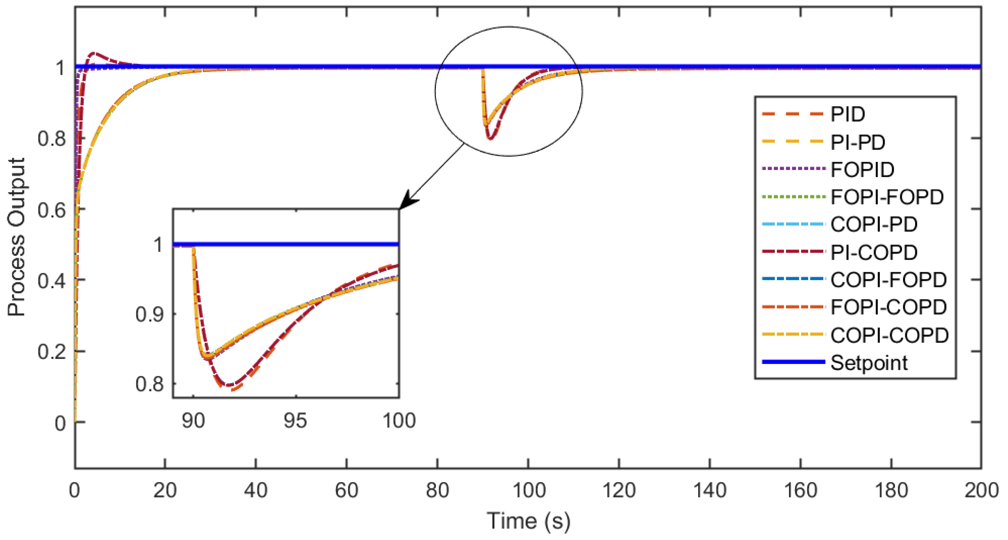
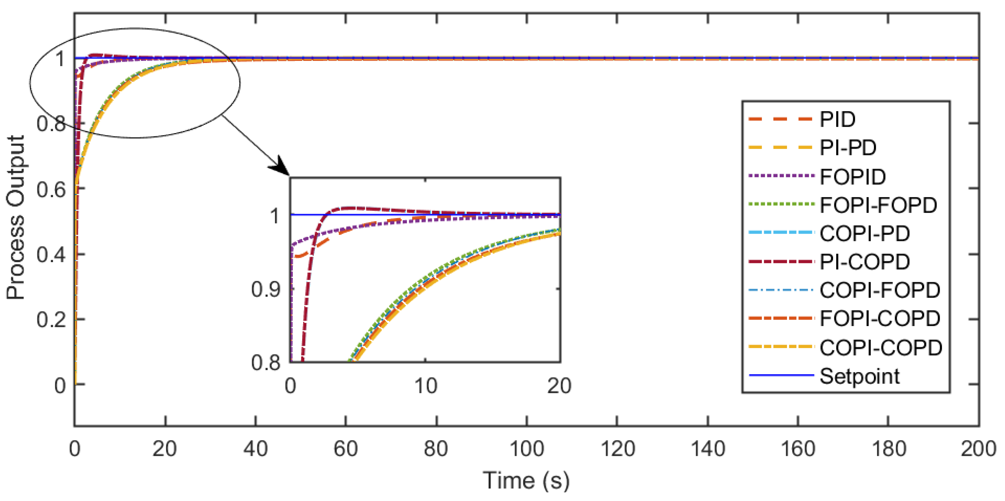
This subsection employs a MATLAB-based simulation to analyse a first-order system using the process model given in Equation (8). The simulation provides valuable insight into dynamic behaviour by inputting relevant system parameters and utilizing MATLAB tools. The transient response parameters are obtained using MATLAB commands. The outcomes of this study contribute significantly to the field and may interest those seeking to enhance their understanding of the topic.

Table 2. Controller parameters and transient response for first-order system.

Controllers	${\mathit{K}}_{\mathit{p}}$	${\mathit{K}}_{\mathit{i}}$	${\mathit{K}}_{\mathit{d}}$	$\mathit{\lambda }$	$\mathit{\mu }$	$\mathit{\beta }$	$\mathit{\gamma }$	OS (%)	Settling Time (${\mathit{t}}_{\mathit{s}}$, Seconds)	Rise Time (${\mathit{t}}_{\mathit{r}}$, Seconds)
PID	17.5	4.12	9.46	-	-	-	-	0.7406	98.3306	66.4899
PI-PD	17.5	4.12	9.46	-	-	-	-	3.7814	117.7727	32.3616
FOPID	17.5	4.12	9.46	0.98	0.02	-	-	0	86.9470	30.8176
FOPI-FOPD	17.5	4.12	9.46	0.98	0.02	-	-	0	138.7361	68.7531
COPI-PD	17.5	4.12	9.46	0.98	-	0.01	-	3.7814	117.7864	32.3687
PI-COPD	17.5	4.12	9.46	-	0.02	-	0.01	3.7642	117.6919	31.7754
COPI-FOPD	17.5	4.12	9.46	0.98	0.02	0.01	-	0.0318	139.1953	69.9659
FOPI-COPD	17.5	4.12	9.46	0.98	0.02	-	0.01	0	138.5352	68.5506
COPI-COPD	17.5	4.12	9.46	0.98	0.02	0.01	0.01	0.0014	138.9981	69.7455

provides a specific time interval for set-point changes, which helps numerically evaluate the controller’s performance. Figure 3 shows the step response of all the controllers followed by each controller structure successfully controlling its output to match the variable set-point changes in Figure 4, and the disturbance-rejection performance is given in Figure 5. The transfer function of the first-order system is given as follows:

$$G\left(s\right)=\frac{1}{5s+1}.$$

(8)

The comparison of the performance of PID and PI-PD controllers through first-order simulations reveals significant differences. Specifically, the PID controller exhibits an overshoot of 0.7406%, with a settling time of 98.3306 s and a rise time of 66.4899 s. In contrast, the PI-PD controller has a higher overshoot of 3.7814%, with a shorter settling time of 117.7727 s and a shorter rise time of 32.3616 s, and while PID controllers exhibit less overshoot and longer settling times, they compensate for this with relatively long rise times. On the other hand, PI-PD controllers prioritize faster rise times at the expense of higher overshoot and longer settling times. The most appropriate selection between these controllers depends on the specific application requirements. It necessitates consideration of the trade-offs between overshoot, settling time, and rise time to achieve the desired system performance.

For fractional controllers, FOPID and FOPI-FOPD controllers exhibit different performance characteristics. The FOPID controller demonstrates a relatively short settling time of 86.9470 s, a fast rise time of 30.8176 s, and an impressive zero overshoot. On the other hand, the FOPI-FOPD controller also boasts zero overshoot but has a long settling time of 138.7361 s and a slow rise time of 68.7531 s. This comparison highlights the trade-offs between the two controllers. The FOPI-FOPD had a slower and steady rise time, which led to zero overshoot, which in turn produced a more stable result (non-oscillatory output). The optimal selection of these sub-regulators depends on the specific application requirements, and it is essential to consider the desired balance between overshoot, settling time, and rise time to achieve optimal system performance. In evaluating complex ordering, each variant has different performance characteristics. The COPI-PD and PI-COPD controllers have overshoot values of 3.7814% and 3.7642%, settling times of 117.7864 s and 117.6919 s, and rise times of 32.3687 s and 31.7754 s, respectively.

The PID controller has less overshoot than the PI-PD controller but has a longer settling time, compromising the overshoot and response time. FOPID controllers prioritize fast response without overshoot, while FOPI-FOPD controllers emphasize stability with more extended settling and rise times. Several violations can be observed in controllers with complex orders. COPI-FOPD minimizes the overshoot, FOPI-COPD emphasizes stability without overshoot, and COPI-COPD achieves minimal overshoot. In contrast, COPI-FOPD has a significantly lower overshoot of 0.0318%, coupled with a longer settling time of 139.1953 s and a rise time of 69.9659 s. FOPI-COPD features zero overshoot, a settling time of 138.5352 s, and a rise time of 68.5506 s, emphasizing stability and a fast response. COPI-COPD achieves a minimum overshoot of 0.0014% with settling and rise times of 138.9981 s and 69.7455 s, respectively.

The set-point changes ensure that the step response reaches its steady-state value. These set-point variations include positive and negative changes, and they assess the controller’s performance effectively. Notably, the proposed COPI-COPD controller outperforms the other controllers, making it more suitable for varying set-point processes.

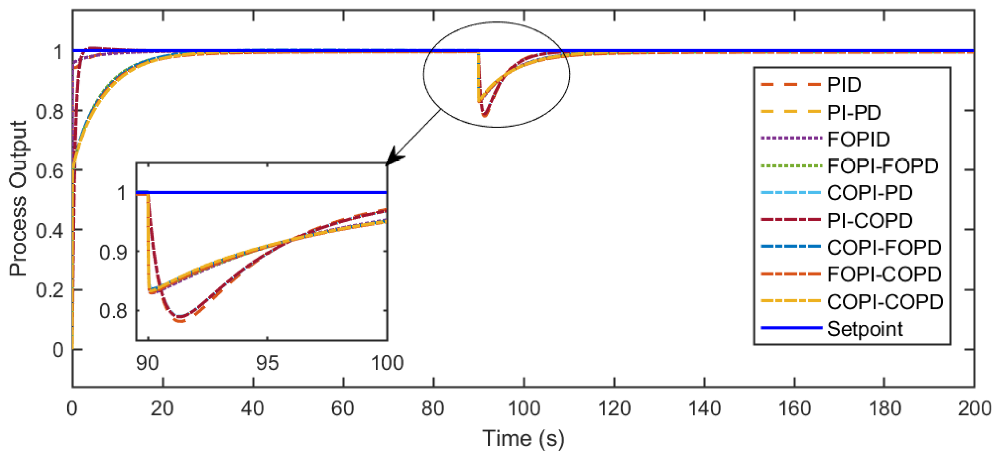
The study involves deliberate exploration of disturbance rejection by injecting a disturbance of 0.5 magnitude into the controller structure for 100 s. This replicates real-life scenarios where external disturbances affect the entire process plant. Figure 5 provides a graphical representation of the adeptness of each controller structure in effectively quelling the disturbance and enabling precise control of the output back to the set point, as depicted in Figure 4’s step response. The empirical validation reveals that the COPI-COPD controller outperforms its competitors, exhibiting better overall performance and emphasizing its robustness and resilience in real-world operational contexts. Complex sequential controllers, particularly the FOPI-COPD, are sturdy tools in set-point tracking, improving control dynamics and higher performance depending on dynamic operating requirements.

3.1.2. Second-Order Process Model

In this section, a simulation based on MATLAB analyses a second-order system. The process model specified in Equation (9) enables systematically exploring the system’s behaviour and dynamics.

Table 3. Controller parameters and transient response for second-order system.

Controllers	${\mathit{K}}_{\mathit{p}}$	${\mathit{K}}_{\mathit{i}}$	${\mathit{K}}_{\mathit{d}}$	$\mathit{\lambda }$	$\mathit{\mu }$	$\mathit{\beta }$	$\mathit{\gamma }$	OS (%)	Settling Time (${\mathit{t}}_{\mathit{s}}$, Seconds)	Rise Time (${\mathit{t}}_{\mathit{r}}$, Seconds)
PID	17.5	4.12	9.46	-	-	-	-	3.663 × 10${-}^7$	116.8035	14.1159
PI-PD	17.5	4.12	9.46	-	-	-	-	0.9225	105.4154	34.6860
FOPID	17.5	4.12	9.46	0.98	0.02	-	-	0	113.8499	30.5718
FOPI-FOPD	17.5	4.12	9.46	0.98	0.02	-	-	0.0547	146.5290	93.6863
COPI-PD	17.5	4.12	9.46	0.98	-	0.01	-	0.9242	105.4284	34.6943
PI-COPD	17.5	4.12	9.46	-	0.02	-	0.01	0.8785	105.2664	33.0961
COPI-FOPD	17.5	4.12	9.46	0.98	0.02	0.01	-	0.1751	147.0024	94.8372
FOPI-COPD	17.5	4.12	9.46	0.98	0.02	-	0.01	0	148.1435	95.0625
COPI-COPD	17.5	4.12	9.46	0.98	0.02	0.01	0.01	0.0076	148.6575	96.3397

provides the numerically evaluating performance of various controllers at a specific time interval for including set-point changes. Figure 6 shows the step response of all the controllers followed by each controller structure successfully controlling its output to match the variable set-point changes in Figure 7, and the disturbance rejection performance is given in Figure 8. The transfer function of the second-order system is given as follows.

$$G\left(s\right)=\frac{2s+1}{s^2+3s+1}.$$

(9)

In the comparison between PID controllers and PI-PD controllers, PID controllers are known for having a very low overshoot value of 3.663 × ${10}^{-7}$%, which indicates precise and stable control. These controllers have a settling time of 116.8035 s and a rise time of 14.1159 s. In contrast, the overshoot value of PI-PD controllers can be as high as 0.9225%, indicating a trade-off between the overshoot and response time. The choice of which controller to use depends on the application’s specific requirements. PID controllers prioritize minimal overshoot and a fast response, while PI-PD controllers offer a faster settling time at the expense of higher overshoot and longer rise time. Fractional-order controllers, particularly FOPID, feature zero overshoot and have a settling time of 113.8499 s and a rise time of 30.5718 s, highlighting their precise and stable control.

It is essential to consider the unique properties of each variant when evaluating complex-order controllers. When it comes to FOPI-FOPD, it has a minimum overshoot value of 0.0547%, a slightly longer settling time of 146.5290 s, and a slightly longer rise time of 93.6863 s, which indicates a trade-off between stability and response time with the proposed COPI-COPD. The choice of these controls is determined by the balance of overshoot, settling time, and rise time required to achieve optimal system performance. Meanwhile, COPI-PD and PI-COPD controllers have similar overshoot values, settling times, and rise times. COPI-FOPD has a low overshoot value of 0.1751%, a long settling time of 147.0024 s, and a long rise time of 94.8372 s. FOPI-COPD shows stability without overshoot, with settling and rise times of 148.1435 s and 95.0625 s. The minimum overshoot value of COPI-COPD is 0.0076%, and the settling time and rise time are 148.6575 s and 96.3397 s, respectively. A comprehensive comparison highlights the multiple trade-offs between these complex-order controllers and emphasizes the need to balance specific application requirements for optimal system performance.

PID controllers are generally more effective in reducing overshoot and providing fast, stable responses. On the other hand, PI-PD controllers tend to have higher overshoot and longer rise times, but they offer faster settling times. FOPID is known for its precise control among fractional controllers, while FOPI-FOPD is renowned for prioritizing stability with minimal compromise in settling and rise times. In the case of complex sequential controllers, each variant has its own characteristics, making it difficult to choose a controller that caters to specific application requirements.

In set-point tracking, the comprehensive evaluation of the figures and table shows that the proposed complex-order controller consistently outperforms its counterpart and performs well. This advantage is not limited to individual cases but extends across target value tracking scenarios. The controller’s subtle adjustments and dynamic responsiveness in complex sequences provide the best overall performance and exceed the capabilities of its controller counterpart. This empirical validation highlights the inherent effectiveness of complex sequential controllers in accurately handling various set-point changes, making them ideal for applications where accuracy and adaptability to varying conditions are important performance criteria. Complex-order controllers have proven to be a transformative force in set-point tracking, promising improved control dynamics and greater adaptability in the face of evolving operational needs.

3.1.3. Third-Order Process Model

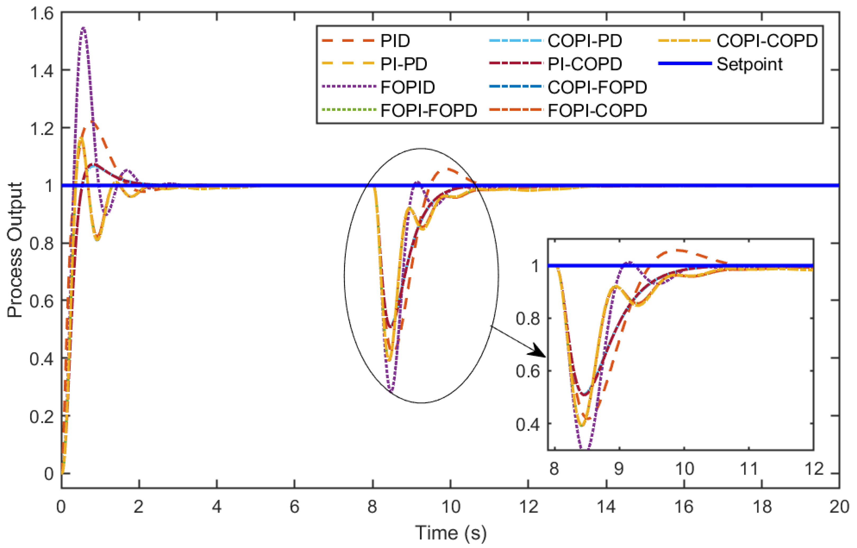
In analysing third-order systems, transfer function models are crucial for simulating and comparing controllers, and their transfer function model is given in Equation (10).

Table 4. Controller parameters and transient response for third-order system.

Controllers	${\mathit{K}}_{\mathit{p}}$	${\mathit{K}}_{\mathit{i}}$	${\mathit{K}}_{\mathit{d}}$	$\mathit{\lambda }$	$\mathit{\mu }$	$\mathit{\beta }$	$\mathit{\gamma }$	OS (%)	Settling Time (${\mathit{t}}_{\mathit{s}}$, Seconds)	Rise Time (${\mathit{t}}_{\mathit{r}}$, Seconds)
PID	2.4532	4.8789	0.3314	-	-	-	-	22.1842	97.8430	17.0763
PI-PD	2.4532	4.8789	0.3314	-	-	-	-	6.7384	88.5320	15.3694
FOPID	2.4532	4.8789	0.3314	0.98	0.02	-	-	54.8152	93.8416	11.3073
FOPI-FOPD	2.4532	4.8789	0.3314	0.98	0.02	-	-	15.8640	94.9228	12.0943
COPI-PD	2.4532	4.8789	0.3314	0.98	-	0.01	-	6.6980	88.5421	15.3753
PI-COPD	2.4532	4.8789	0.3314	-	0.02	-	0.01	7.3362	88.0580	15.3340
COPI-FOPD	2.4532	4.8789	0.3314	0.98	0.02	0.01	-	16.5639	94.7933	12.0374
FOPI-COPD	2.4532	4.8789	0.3314	0.98	0.02	-	0.01	15.8146	94.8964	12.0969
COPI-COPD	2.4532	4.8789	0.3314	0.98	0.02	0.01	0.01	16.5141	94.7665	12.04

provides the numerically evaluated performance of various controllers at a specific time interval, including set-point changes and disturbance rejection analysis. Figure 9 shows the step response of all the controllers followed by each controller structure successfully controlling its output to match the variable set-point changes in Figure 10, and the disturbance rejection performance is given in Figure 11. By focusing on the controller’s transient response characteristics, transfer function models can provide insight into the controller’s performance under varying conditions. This approach allows for a nuanced study of the controller’s behaviour and provides a systematic means of recognizing the controller’s effectiveness in tuning the system response. Therefore, transfer function models represent a methodologically rigorous path that allows for a comprehensive investigation and evaluation of controller performance within the dynamic landscape of third-order systems. The transfer function of the third-order system is given as follows.

$$G\left(s\right)=\frac{400}{s^3+30s^2+200s}.$$

(10)

PID controllers are known for their fast response time but have a significant overshoot of 22.1842%, allowing large deviations from the set point. The PI-PD controller, on the other hand, achieves slightly longer settling and rise times but reaches a lower overshoot value of 6.7384%, resulting in improved control accuracy. This trade-off between faster response and higher overshoot for PID controllers versus precise control of PI-PD controllers with slightly longer settling and rise times is noteworthy. Regarding fractional-order regulators, FOPID controllers can provide potentially faster response times but have a high overshoot value of 54.8152%. The FOPI-FOPD controller, with an overshoot value of 15.8640% and a slight compromise in rise time, is a better option for those seeking the balance between overshoot and the response time. COPI-PD and PI-COPD controllers have similar overshoot values but different settling and rise times for complex-order controllers. COPI-FOPD increases settling time to minimize the overshoot to 16.5639%, while FOPI-COPD emphasizes stability with a slightly reduced overshoot value of 15.8146%. COPI-COPD, on the other hand, minimizes the overshoot to 16.5639%.

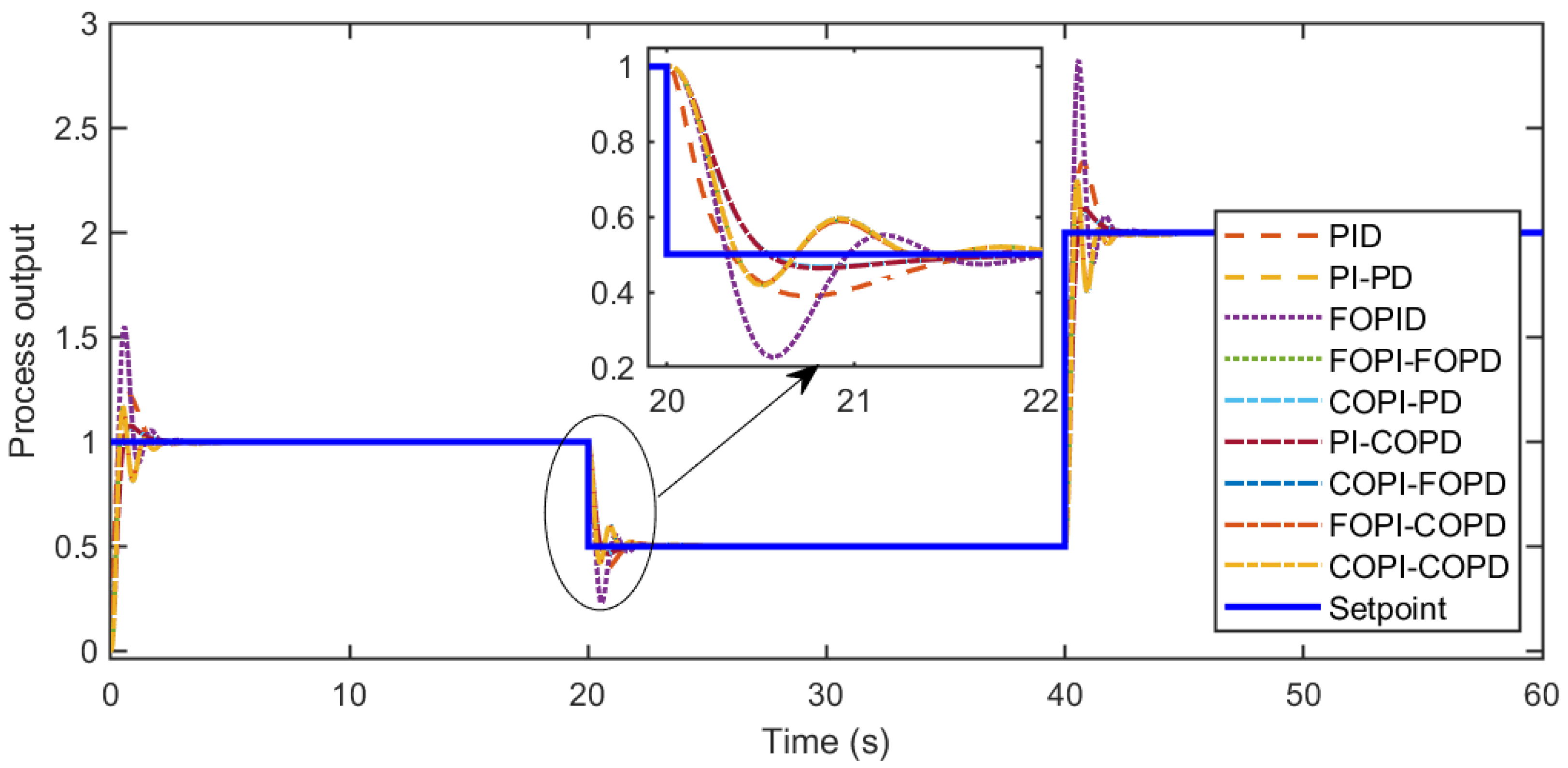
Set-point tracking involves adjusting input values at various intervals to evaluate the controller’s robustness under different conditions. Strategic analysis is carried out by changing the initial set points, starting at 1 at time 0, moving to 0.5 at 20 s, and progressing to 2 at 40 s while keeping track of positive and negative changes. This test bench provides a comprehensive analysis of the controller’s functionality. This step response cleverly adjusts its output to match the specified set-point change, highlighting the superior overall performance of the proposed complex slave controller.

The complex slave controller consistently outperforms comparable controllers with its high adaptability and accuracy, making it ideal for applications where control and adaptability to varying conditions are key performance indicators. Complex-order controllers have proven indispensable partners in set-point tracking, providing improved control dynamics and higher performance standards in the face of dynamic operating requirements. The comprehensive evaluation of disturbance rejection involved the construction of a deliberate and pertinent scenario. In this scenario, an intentional disturbance value of 2 was injected into the controller structure after 8 s.

These simulation results accurately mimic real-life situations where disturbances can permeate the entirety of a process plant. The intricate dynamics of this scenario are depicted in Figure 11, where each control structure adeptly navigates the challenges posed by disturbances and dynamically adjusts the output back to the set point. This observed response aligns seamlessly with the step response illustrated in Figure 9. The proposed complex-order controller consistently emerges as the front-runner in this evaluation, outperforming its competitors with a demonstrable superiority in effectively managing and suppressing disturbances. The nuanced and resilient performance of the complex-order controller underscores its efficacy in maintaining overall system control amidst external disruptions. This empirical evidence not only highlights the specific prowess of the complex-order controller in disturbance rejection but also positions it as the optimal choice for applications where superior disturbance management and sustained system control are paramount performance criteria. The complex-order controller is a robust solution, offering enhanced control dynamics and a heightened ability to contend with real-world disturbances within dynamic operational environments.

3.2. Experimental Study

This section provides a detailed discussion of real-time flow and pressure process plant results, including their schematics and operating characteristics. It is worth noting that a delay by a first-order transfer function characterizes both plants. However, an obstacle arises when attempting to derive the transient response using MATLAB commands, as discussed in the previous section. The resulting transfer functions exhibit irregularities that make them non-causal and unstable. The solution to this challenge is achieved by applying the Pade approximation, where the problem is effectively reduced as the order of the numerator is now equal to or exceeds the order of the denominator. This adjustment ensures the stability and causality of the system, overcoming the limitations associated with non-causal systems, which are considered physically infeasible due to their dependence on inputs from future temporary cases.

3.2.1. Flow Process Model

The experimental setup and piping and instrument diagram (P&ID) of the real-time flow process plant are illustrated in Ref. [40]. Within this system, the process tank, VE 420, has a capacity of 100 litres and receives liquid from tank VE 410 with the assistance of a centrifugal pump P412. The liquid level within VE 420 is effectively controlled by a hand valve HV 420, while the process control valve FCV 413 ensures a consistent flow at the designated level. A pressure transmitter FT 413 measures and regulates the flow, providing digital voltage signals within the range of 0 to 5 V.

These voltage signals are then directed to the pressure-indicating controller FIC 413, which transmits the control signal to the host PC through dedicated I/O interface boards. This integration allows for real-time monitoring and control of the flow process, showcasing a comprehensive and sophisticated system architecture, from the open-loop response of the flow process followed by its numerical analysis in

Table 5. Controller parameters and transient response for real-time flow process plant.

Controllers	${\mathit{K}}_{\mathit{p}}$	${\mathit{K}}_{\mathit{i}}$	${\mathit{K}}_{\mathit{d}}$	$\mathit{\lambda }$	$\mathit{\mu }$	$\mathit{\beta }$	$\mathit{\gamma }$	OS (%)	Settling Time (${\mathit{t}}_{\mathit{s}}$, Seconds)	Rise Time (${\mathit{t}}_{\mathit{r}}$, Seconds)
PID	1	1	0.1	-	-	-	-	6.1045 × ${10}^{-5}$	237.6946	78.3350
PI-PD	1	1	0.1	-	-	-	-	0	240.7698	80.6822
FOPID	1	1	0.1	0.98	0.02	-	-	1.2636 × ${10}^{-4}$	239.3677	79.5915
FOPI-FOPD	1	1	0.1	0.98	0.02	-	-	0	241.8704	81.9465
COPI-PD	1	1	0.1	0.98	-	0.01	-	1.2549 × ${10}^{-4}$	239.3861	79.6018
PI-COPD	1	1	0.1	-	0.02	-	0.01	1.2648 × ${10}^{-4}$	239.3679	79.5916
COPI-FOPD	1	1	0.1	0.98	0.02	0.01	-	2.6519 × ${10}^{-4}$	241.5152	82.1655
FOPI-COPD	1	1	0.1	0.98	0.02	-	0.01	0	241.8741	81.9517
COPI-COPD	1	1	0.1	0.98	0.02	0.01	0.01	2.3946 × ${10}^{-4}$	241.5194	82.1699

. The mathematical model derivation for the process plant involves analysing the open-loop step response characteristics. These characteristics encompass essential information about the behaviour and dynamics of the process, including parameters such as the process gain (K), process dead time ($L_p$), and process time constant (T). In this experimentation, an open-loop step response is performed for the flow process, yielding the following plant dynamics: $K=0.072$, $L_p=3$, and $T=0.126$. Utilizing the characteristic equation for a first-order plus dead-time system, the process model for the flow process plant is established based on the acquired plant dynamics. The transfer function of the process is given as

$$G\left(s\right)=\frac{K}{1+Ts}{e}^{-s{L}_p}=\frac{0.072}{0.126s+1}{e}^{-3s}.$$

(11)

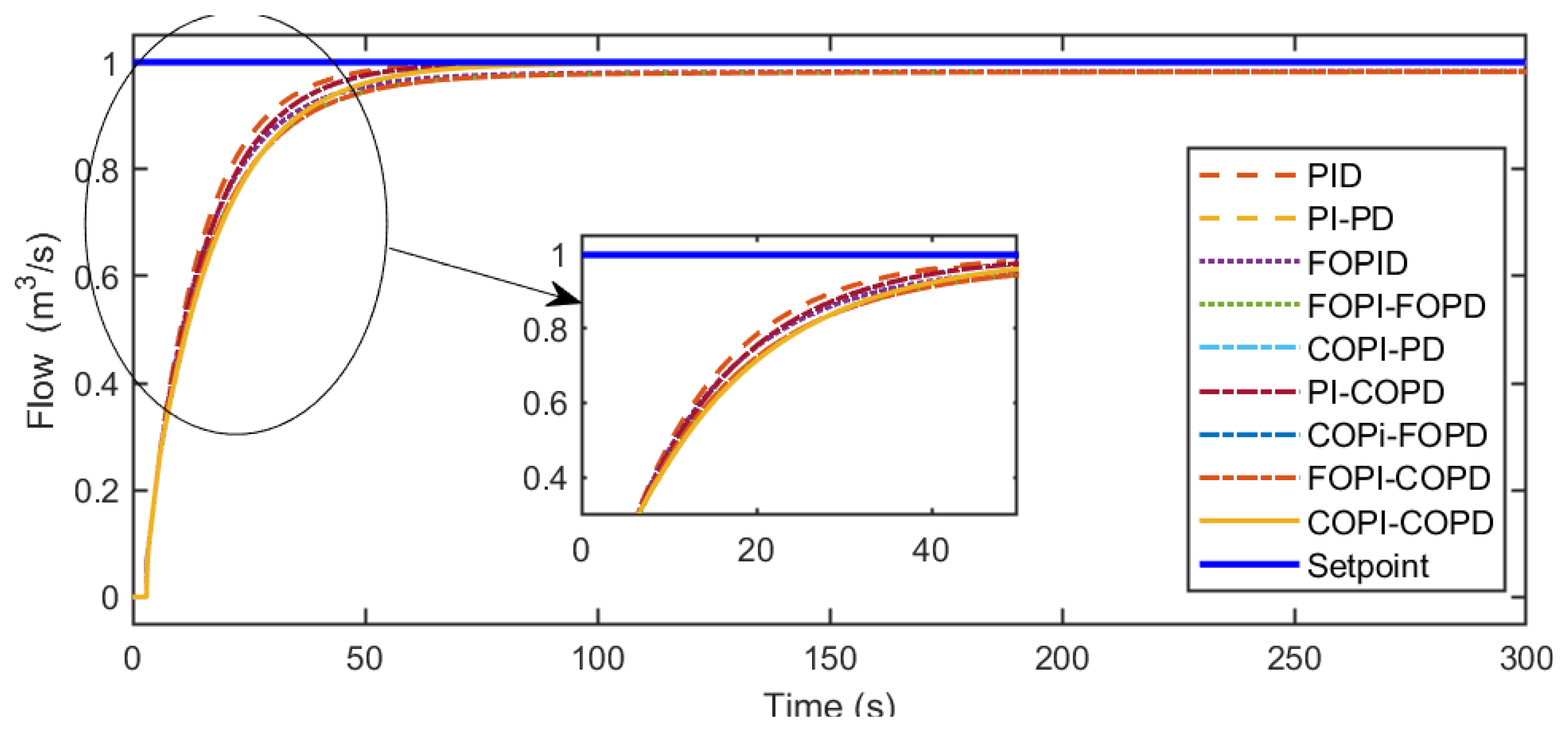
To ensure the system’s stability, the plant is operated by controllers, which employ the same methodology as the previous system. However, fractional and complex-order controllers have been added to compare with other controllers. The parameters of these controllers and the step response and transient response characteristics are presented in the table and figure below. These figures provide a comprehensive overview of the control system’s performance. Figure 12, Figure 13 and Figure 14 show the step, set-point tracking, and disturbance rejection responses of all the controllers.

The comparison of the traditional controller to the experimental analysis reveals that the PID controller exhibits an overshoot of 6.1045 $\times {10}^{-5}$%, which is higher than the PI-PD controller, which achieves zero overshoot. The PID controllers have smaller rise and settling time values, but it does not necessarily mean a better performance, as the overshoot is a crucial factor when evaluating control quality. In the case of fractional controllers, the comparison between FOPID and FOPI-FOPD shows that FOPI-FOPD is better than FOPID as it has zero overshoot. However, it has a lower settling time of 239.3677 s and a rise time value of 79.5915 s, which is smaller for FOPID. FOPI-FOPD shows excellent interference rejection performance with no overshoot. The analysis conducted on complex sequential controllers such as COPI-PD, PI-COPD, COPI-FOPD, FOPI-COPD, and COPI-COPD revealed that FOPI-COPD showed superior performance compared to the others. FOPI-COPD achieved a settling time of 241.8741 s with a rise time of only 81.9517 s and no overshoot, indicating high accuracy and stability. These results set FOPI-COPD apart from another similar controller that exhibits non-zero overshoot values, emphasizing its exceptional performance in achieving precise and stable control.

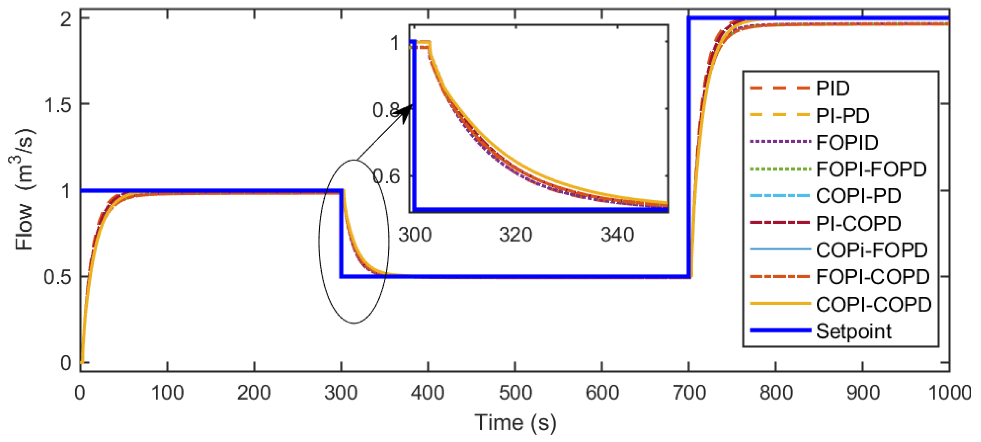
These performance comparisons highlight the importance of considering multiple performance parameters while assessing controllers and suggest that traditional controllers, such as PID, may suffer from overshoot. In contrast, fractional controllers like FOPI-FOPD and FOPI-COPD offer improved overshoot minimization, settling time, and rise time. These findings suggest that FOPI-COPD is a compelling option for applications where precise control is paramount. A salient observation concentrates from this comprehensive study, with the proposed complex-order controller consistently emerging as the epitome of effectiveness, outperforming its competitors in terms of overall performance. This consistent superiority is a recurring theme throughout the configuration value tracking scenario, with the nuanced adaptability showcased by the complex-order controller underscoring its prowess in navigating diverse configuration changes. Therefore, it solidifies its status as the optimal choice for applications where precise control and adaptability to varied configurations are pivotal performance benchmarks. The complex-order controller establishes itself as a stalwart in configuration value tracking, promising enhanced control dynamics and an elevated performance standard in the face of evolving operational requirements.

In the context of disturbance rejection, a real-world analysis is presented where a deliberate disturbance value of 6 is introduced into the controller structure after 150 s. This mirrors the dynamic nature of external disturbances in a process plant. Figure 14 illustrates the intricacies of this scenario, providing a clear visual representation of the proficiency of each controller structure in mitigating the effects of disturbances. These controllers demonstrate their adeptness through dynamic adjustments to the output, aligning it with the set point, as shown in the step response diagram captured in Figure 12. Notably, the proposed complex-order controller consistently outperforms competitors in interference suppression, showcasing superior overall performance. All of the above consistently better performances over other controllers underscore the robustness of the proposed complex-order controllers in dealing with disturbances, positioning them as the optimal choice for applications where disturbance rejection is a critical performance criterion. The empirical evidence from this evaluation highlights the potential of complex-order controllers in providing resilient and effective solutions for managing external disturbances, further solidifying their candidacy for applications where precision and adaptability to disturbances are paramount considerations.

3.2.2. Pressure Process Model

The schematic diagram and piping and instrument diagram of the real-time pressure process plant illustrated in Refs. [40,41,42], provide a comprehensive overview of the system’s operational dynamics. The pressure system is centred around the VL 202 buffer tank, specially designed to withstand the high pressure of up to 10 bar supplied by the centralized air compression system. The HV 202 manual valve enables precise control over the pressure. In contrast, the PCV 202 process control valve ensures that the pressure is constantly maintained at the desired level, allowing for a smooth and efficient operation. The PT 202 pressure transmitter facilitates accurate pressure monitoring by converting pressure values into digital voltage signals ranging from 0 to 5 V.

The PIC 202 pressure indicator controller relays this voltage signal to the host PC via dedicated I/O interface cards, enabling real-time pressure process monitoring and control. This showcases a complex and comprehensive system architecture. The PT 202 pressure transmitter and PIC 202 pressure indicator controller suit various industries where precise pressure measurements are critical to operations. This technology ensures accurate and reliable pressure monitoring, ensuring smooth and efficient operations. Using the open-loop response of the pressure process followed by its numerical analysis in

Table 6. Controller parameters and transient response for real-time pressure process plant.

Controllers	${\mathit{K}}_{\mathit{p}}$	${\mathit{K}}_{\mathit{i}}$	${\mathit{K}}_{\mathit{d}}$	$\mathit{\lambda }$	$\mathit{\mu }$	$\mathit{\beta }$	$\mathit{\gamma }$	OS (%)	Settling Time (${\mathit{t}}_{\mathit{s}}$, Seconds)	Rise Time (${\mathit{t}}_{\mathit{r}}$, Seconds)
PID	0.5	0.5	−0.01	-	-	-	-	6.5841	163.0095	18.5776
PI-PD	0.5	0.5	−0.01	-	-	-	-	0.3905	175.9587	38.7020
FOPID	0.5	0.5	−0.01	0.98	0.02	-	-	4.0610	162.1264	25.0510
FOPI-FOPD	0.5	0.5	−0.01	0.98	0.02	-	-	0.2565	178.9595	40.4344
COPI-PD	0.5	0.5	−0.01	0.98	-	0.01	-	0.2876	176.0390	38.7466
PI-COPD	0.5	0.5	−0.01	-	0.02	-	0.01	7.5495 × ${10}^{-12}$	177.5542	83.0930
COPI-FOPD	0.5	0.5	−0.01	0.98	0.02	0.01	-	0	180.4267	86.5732
FOPI-COPD	0.5	0.5	−0.01	0.98	0.02	-	0.01	0	180.2877	84.9259
COPI-COPD	0.5	0.5	−0.01	0.98	0.02	0.01	0.01	2.1894 × ${10}^{-11}$	180.4000	86.4863

, the transfer function of the process is given as

$$G\left(s\right)=\frac{0.866}{1.365s+1}{e}^{-s}.$$

(12)

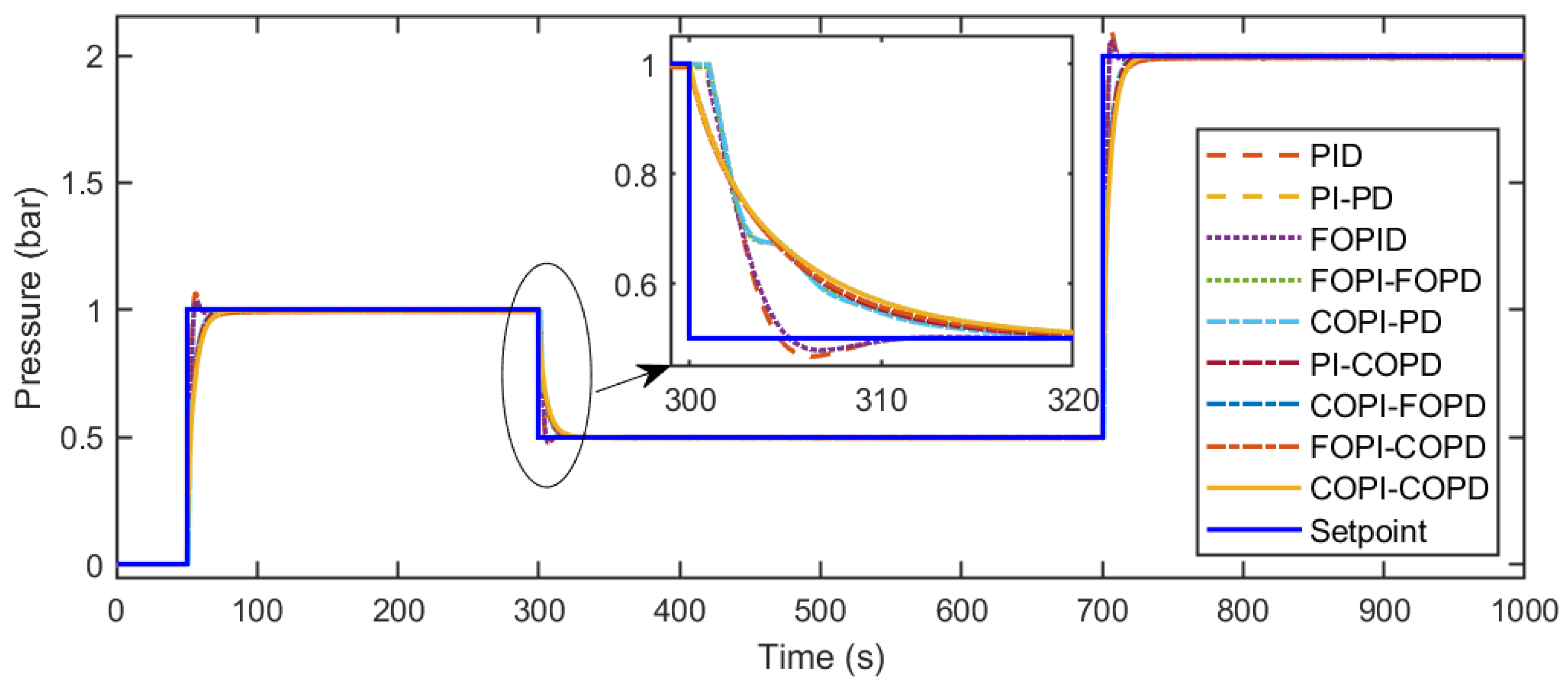
Figure 15, Figure 16 and Figure 17 show the step, set-point tracking, and disturbance-rejection responses of all the controllers in the pressure process plant. Controllers are employed to operate the plant to assess the system’s stability, which is consistent with past methods and includes the addition of fractional and complex order controllers for comparison purposes. The resulting table and figure showcase the parameters, step response, and transient response characteristics, thoroughly assessing the control system’s performance. The simulation study results revealed that the PID controller demonstrated a significant overshoot of 6.5841% with a settling time of 163.0095 s and a rise time of 18.5776 s. Conversely, the PI-PD controller exhibited a considerably lower overshoot of 0.3905%, albeit with a slightly longer settling time of 175.9587 s and a longer rise time of 38.7020 s. This comparison demonstrates that the PID controller trades off higher overshoot and faster settling and rise times. In contrast, the PI-PD controller has slightly longer settling and rise times but minimal overshoot. The optimal choice of these controllers depends on the specific application requirements, where it is essential to balance the overshoot and response time to optimize the system performance.

In the fractional controllers, to evaluate the performance of FOPID and FOPI-FOPD controllers, the FOPID controller demonstrates a significant overshoot of 4.0610%, accompanied by a settling time of 162.1264 s and a rise time of 25.0510 s. In contrast, the FOPI-FOPD controller presents a considerably reduced overshoot, amounting to 0.2565%, albeit with a slightly longer settling time of 178.9595 s and a higher rise time of 40.4344 s. The comparison between the two controllers sheds light on the trade-off between the FOPID controller’s faster settling time and shorter rise time, yet higher overshoot, and the FOPI-FOPD controller’s minimized overshoot, prioritizing stability at the expense of marginally longer settling and rise times. The selection of the fractional controller depends on the specific application’s needs, which requires careful consideration of the trade-off between the overshoot and response time for effective control system design.

In evaluating complex-order controllers, each variant has demonstrated unique performance characteristics. COPI-PD has exhibited a moderate overshoot of 0.2876%, with a settling time of 176.0390 s and a rise time of 38.7466 s. PI-COPD has shown a nearly imperceptible overshoot of 7.5495 $\times {10}^{-12}$%, achieving a settling time of 177.5542 s and a rise time of 83.0930 s. COPI-FOPD has excelled in overshoot elimination with a value of zero percent, coupled with a settling time of 180.4267 s and a rise time of 86.5732 s. FOPI-COPD has emerged as a standout performer, exhibiting zero percent overshoot, a settling time of 180.2877 s, and a rise time of 84.9259 s, making it the preferred choice. Although COPI-COPD has also achieved a negligible overshoot of $2.1894 \times {10}^{-11}$% with a settling time of 180.4 s and a rise time of 86.4863 s, the comprehensive assessment positions FOPI-COPD as the superior controller, showcasing optimal performance across the overshoot, settling time, and rise time among the complex-order controllers evaluated.

After a comprehensive examination, a clear trend emerges, indicating that the proposed complex sequential controllers, specifically the FOPI-COPD, consistently surpass their competitors and demonstrate the pinnacle of overall performance. This recurring advantage is not a singular event but a recurring theme throughout various set-point tracking scenarios. The outstanding performance of complex sequencers, particularly the FOPI-COPD, provides substantial evidence of their adeptness in controlling changes in diverse set points. This empirical validation positions these controllers as the foremost choice for applications prioritizing accuracy, adaptability, and superior overall performance. By nature, complex sequential controllers, especially the FOPI-COPD, have proven to be robust tools in set-point tracking, improving control dynamics and ensuring higher performance based on dynamic operating requirements.

As per the analysis conducted on the array of control structures, the FOPI-COPD controller consistently emerges as the best performing controller, showcasing superior overall performance compared to its counterparts. This recurring trend underscores the robust interference suppression capabilities inherent in the FOPI-COPD controller. The empirical evidence from this analysis positions the FOPI-COPD controller as the optimal choice for applications where minimizing interference effects is a crucial performance criterion. This observation emphasizes the FOPI-COPD controller’s efficacy in mitigating disturbances and underscores its suitability for real-world scenarios demanding precise interference suppression and control.

4. Conclusions

Introducing complex-order PI-PD controllers is a promising approach to enhance control performance in real-time process plants. This innovative strategy integrates complex orders, utilizes advanced algorithms and techniques, and addresses critical issues such as transient response, overshoot, stability, and robustness. Moving from traditional integer order to complex order adds nuance and precision to the control approach, encouraging the development of new controllers. Implementing complex-order PI-PD controllers requires careful hardware selection and seamless integration. This approach effectively manages industrial environments’ complexity, leading to improved control dynamics and increased operational efficiency in dynamic industrial processes. This pioneering integration underscores our dedication to advancing control techniques and marks a positive step towards achieving optimal operational efficiency. Leveraging complex-order PI-PD controllers’ advanced features, we lead the way in technological innovation, bringing new precision and adaptability to dynamic situations in industrial control systems. Optimal performance in complex order controllers will be achieved by incorporating a thorough optimization and testing phase in the deployment process, which is the future direction of this research. Controllers can be subjected to various parameters to identify the most efficient configuration, which requires careful evaluation of different characteristics.

References

- Lloyds Raja, G.; Ali, A. New PI-PD controller design strategy for industrial unstable and integrating processes with dead time and inverse response. J. Control Autom. Electr. Syst. 2021, 32, 266–280. [Google Scholar] [CrossRef]
- Onat, C. A new design method for PI–PD control of unstable processes with dead time. ISA Trans. 2019, 84, 69–81. [Google Scholar] [CrossRef] [PubMed]
- Du, X.; Wang, J.; Jegatheesan, V.; Shi, G. Dissolved oxygen control in activated sludge process using a neural network-based adaptive PID algorithm. Appl. Sci. 2018, 8, 261. [Google Scholar] [CrossRef]
- Feng, Y.; Wu, M.; Chen, X.; Chen, L.; Du, S. A fuzzy PID controller with nonlinear compensation term for mold level of continuous casting process. Inf. Sci. 2020, 539, 487–503. [Google Scholar] [CrossRef]
- Bingi, K.; Ibrahim, R.; Noh Karsiti, M.; Miya Hassan, S. Fractional-order PI-PD control of real-time pressure process. Prog. Fract. Differ. Appl. 2020, 6, 289–299. [Google Scholar]
- George, M.A.; Elwakil, A.S.; Allagui, A.; Psychalinos, C. Design of Complex-Order PI/PID Speed Controllers and its FPAA Realization. IEEE Access 2023. [Google Scholar] [CrossRef]
- Bao, Y.; Cheng, P.; Pham, K.; Blasch, E.; Shen, D.; Tian, X.; Chen, G. PID-based automatic gain control for satellite transponder under partial-time partial-band AWGN jamming. In Proceedings of the Sensors and Systems for Space Applications XVI, Orlando, FL, USA, 30 April–5 May 2023; SPIE: Bellingham, WA, USA, 2023; Volume 12546, pp. 61–68. [Google Scholar]
- Das, D.; Chakraborty, S.; Raja, G.L. Enhanced dual-DOF PI-PD control of integrating-type chemical processes. Int. J. Chem. React. Eng. 2022. [Google Scholar] [CrossRef]
- Peker, F.; Kaya, I. Identification and real time control of an inverted pendulum using PI-PD controller. In Proceedings of the 2017 IEEE 21st International Conference on System Theory, Control and Computing (ICSTCC), Sinaia, Romania, 19–21 October 2017; pp. 771–776. [Google Scholar]
- Muresan, C.I.; Copot, C.; Birs, I.; De Keyser, R.; Vanlanduit, S.; Ionescu, C.M. Experimental validation of a novel auto-tuning method for a fractional order PI controller on an UR10 robot. Algorithms 2018, 11, 95. [Google Scholar] [CrossRef]
- Xu, L.; Song, B.; Cao, M.; Xiao, Y. A new approach to optimal design of digital fractional-order PIλDμ controller. Neurocomputing 2019, 363, 66–77. [Google Scholar] [CrossRef]
- Dash, P.; Saikia, L.C.; Sinha, N. Flower pollination algorithm optimized PI-PD cascade controller in automatic generation control of a multi-area power system. Int. J. Electr. Power Energy Syst. 2016, 82, 19–28. [Google Scholar] [CrossRef]
- Mondal, R.; Dey, J. A novel design methodology on cascaded fractional order (FO) PI-PD control and its real time implementation to Cart-Inverted Pendulum System. ISA Trans. 2022, 130, 565–581. [Google Scholar] [CrossRef] [PubMed]
- Devan, P.; Hussin, F.A.; Ibrahim, R.B.; Bingi, K.; Nagarajapandian, M.; Assaad, M. An arithmetic-trigonometric optimization algorithm with application for control of real-time pressure process plant. Sensors 2022, 22, 617. [Google Scholar] [CrossRef] [PubMed]
- Padhy, S.; Panda, S. A hybrid stochastic fractal search and pattern search technique based cascade PI-PD controller for automatic generation control of multi-source power systems in presence of plug in electric vehicles. CAAI Trans. Intell. Technol. 2017, 2, 12–25. [Google Scholar] [CrossRef]
- Shanthini, C.; Devi, V.K.; Rajendran, S.; Jena, D. Comparative analysis of PID, I-PD and fractional order PI-PD for a DC-DC converter. In Proceedings of the 2022 IEEE North Karnataka Subsection Flagship International Conference (NKCon), Vijayapura, India, 20–21 November 2022; pp. 1–5. [Google Scholar]
- Singh, V.K.; Sharma, S.; Padhy, P.K. Controlling of AVR Voltage and Speed of DC Motor Using Modified PI-PD Controller. In Proceedings of the 2018 2nd IEEE International Conference on Power Electronics, Intelligent Control and Energy Systems (ICPEICES), Delhi, India, 22–24 October 2018; pp. 858–863. [Google Scholar]
- Singh, V.K.; Padhy, P. A new approach to PI-PD controller Design using modified relay feedback. In Proceedings of the 2018 International Conference on Power Energy, Environment and Intelligent Control (PEEIC), Greater Noida, India, 13–14 April 2018; pp. 349–353. [Google Scholar]
- Muresan, C.I.; Dulf, E.H.; Both, R. Vector-based tuning and experimental validation of fractional-order PI/PD controllers. Nonlinear Dyn. 2016, 84, 179–188. [Google Scholar] [CrossRef]
- Roong, A.S.C.; Shin-Homg, C.; Said, M.A.B. Position control of a magnetic levitation system via a PI-PD control with feedforward compensation. In Proceedings of the 2017 IEEE 56th Annual Conference of the Society of Instrument and Control Engineers of Japan (SICE), Kanazawa, Japan, 19–22 September 2017; pp. 73–78. [Google Scholar]
- Ozan, G.; Nusret, T. Voltage control at building integrated photovoltaic and wind turbine system with PI-PD controller. Avrupa Bilim ve Teknoloji Dergisi 2020, 18, 992–1003. [Google Scholar]
- Peram, M.; Mishra, S.; Vemulapaty, M.; Verma, B.; Padhy, P.K. Optimal PI-PD and I-PD controller design using cuckoo search algorithm. In Proceedings of the 2018 IEEE 5th International Conference on Signal Processing and Integrated Networks (SPIN), Noida, India, 22–23 February 2018; pp. 643–646. [Google Scholar]
- Irshad, M.; Ali, A. Robust PI-PD controller design for integrating and unstable processes. IFAC-PapersOnLine 2020, 53, 135–140. [Google Scholar] [CrossRef]
- Ali, H.I.; Saeed, A.H. Robust Tuning of PI-PD Controller for Antilock Braking System. Al-Nahrain J. Eng. Sci. 2017, 20, 983–995. [Google Scholar]
- Merrikh-Bayat, F. An iterative LMI approach for H∞ synthesis of multivariable PI/PD controllers for stable and unstable processes. Chem. Eng. Res. Des. 2018, 132, 606–615. [Google Scholar] [CrossRef]
- Zou, H.; Li, H. Improved PI-PD control design using predictive functional optimization for temperature model of a fluidized catalytic cracking unit. ISA Trans. 2017, 67, 215–221. [Google Scholar] [CrossRef]
- Alyoussef, F.; Kaya, I. Simple PI-PD tuning rules based on the centroid of the stability region for controlling unstable and integrating processes. ISA Trans. 2023, 134, 238–255. [Google Scholar] [CrossRef]
- Bingi, K.; Ibrahim, R.; Karsiti, M.N.; Hassan, S.M.; Harindran, V.R. Real-time control of pressure plant using 2DOF fractional-order PID controller. Arab. J. Sci. Eng. 2019, 44, 2091–2102. [Google Scholar] [CrossRef]
- Zheng, M.; Huang, T.; Zhang, G. A new design method for PI-PD control of unstable fractional-order system with time delay. Complexity 2019, 2019, 1–12. [Google Scholar] [CrossRef]
- Ranjbaran, K.; Tabatabaei, M. Fractional order [PI],[PD] and [PI][PD] controller design using Bode’s integrals. Int. J. Dyn. Control 2018, 6, 200–212. [Google Scholar] [CrossRef]
- Ozyetkin, M.M. A simple tuning method of fractional order PIλ-PDμ controllers for time delay systems. ISA Trans. 2018, 74, 77–87. [Google Scholar] [CrossRef] [PubMed]
- Ozyetkin, M.M.; Onat, C.; Tan, N. PI-PD controller design for time delay systems via the weighted geometrical center method. Asian J. Control 2020, 22, 1811–1826. [Google Scholar] [CrossRef]
- Dakua, B.K.; Ansari, M.S.; Bhoi, S.; Pati, B.B. Design of PI λ- PD μ Controller for Industrial Unstable and Integrating Processes with Time Delays. In Proceedings of the International Symposium on Sustainable Energy and Technological Advancements, Shillong, India, 24–25 February 2023; Springer: New York, NY, USA, 2023; pp. 261–275. [Google Scholar]
- Nema, S.; Padhy, P.K. MPSO PI-PD controller for SISO processes. In Proceedings of the 2015 IEEE 9th International Conference on Intelligent Systems and Control (ISCO), Coimbatore, India, 9–10 January 2015; pp. 1–6. [Google Scholar]
- Guedri, B.; Chaari, A. Design and optimal tuning of fractional order αIP-PD controller for unstable and integrating processes. In Proceedings of the 2017 IEEE International Conference on Advanced Systems and Electric Technologies (IC_ASET), Hammamet, Tunisia, 14–17 January 2017; pp. 216–220. [Google Scholar]
- Sengupta, S.; Karan, S.; Dey, C. MSP designing with optimal fractional PI–PD controller for IPTD processes. Chem. Prod. Process Model. 2022. [Google Scholar] [CrossRef]
- Upadhyaya, A.; Gaur, P. Speed Control of Hybrid Electric Vehicle using cascade control of Fractional order PI and PD controllers tuned by PSO. In Proceedings of the 2021 IEEE 18th India Council International Conference (INDICON), Guwahati, India, 19–21 December 2021; pp. 1–6. [Google Scholar]
- Bingi, K.; Ibrahim, R.; Karsiti, M.N.; Hassan, S.M.; Harindran, V.R. Fractional-Order Systems and PID Controllers; Springer: Cham, Switzerland, 2020; Volume 264. [Google Scholar]
- Abdulwahhab, O.W. Design of a complex fractional order PID controller for a first order plus time delay system. ISA Trans. 2020, 99, 154–158. [Google Scholar] [CrossRef] [PubMed]
- Fawwaz, M.A.; Bingi, K.; Ibrahim, R.; Devan, P.A.M.; Prusty, B.R. Design of pidd α controller for robust performance of process plants. Algorithms 2023, 16, 437. [Google Scholar] [CrossRef]
- Devan, P.A.M.; Ibrahim, R.; Omar, M.; Bingi, K.; Abdulrab, H. A novel hybrid harris hawk-arithmetic optimization algorithm for industrial wireless mesh networks. Sensors 2023, 23, 6224. [Google Scholar] [CrossRef] [PubMed]
- Selvam, A.M.D.P.; Hussin, F.A.; Ibrahim, R.; Bingi, K.; Nagarajapandian, M. Optimal Fractional-Order Predictive PI Controllers: For Process Control Applications with Additional Filtering; Springer Nature: Singapore, 2022. [Google Scholar]
Figure 1.
Block diagram of integer and fractional PID controllers.
Figure 2.
Block diagram of a PI-PD, FOPI-PD, and COPI-PD controllers.
Figure 3.
First-order process model’s step response with compared controllers.
Figure 4.
First-order process model’s tracking response with compared controllers.
Figure 5.
First-order process model’s disturbance response with compared controllers.
Figure 6.
Second-order process model’s step response with compared controllers.
Figure 7.
Second-order process model’s tracking response with compared controllers.
Figure 8.
Second-order process model’s disturbance response with compared controllers.
Figure 9.
Third-order process model’s step response with compared controllers.
Figure 10.
Third-order process model’s tracking response with compared controllers.
Figure 11.
Third-order process model’s disturbance response with compared controllers.
Figure 12.
Flow process model’s step response with compared controllers.
Figure 13.
Flow process model’s tracking response with compared controllers.
Figure 14.
Flow process model’s disturbance response with compared controllers.
Figure 15.
Pressure process model’s step response with compared controllers.
Figure 16.
Pressure process model’s tracking response with compared controllers.
Figure 17.
Pressure process model’s disturbance response with compared controllers.