Elastic and Dielectric Evaluation of the Piezoelectric Response of Ferroelectrics Using Unpoled Ceramics

Abstract

The evaluation of the piezoelectric properties of ferroelectric ceramics generally has a high level of uncertainty, due to incomplete poling, porosity, domain wall clamping and other effects. In addition, the poling process is often difficult and dangerous, due to the risk of breaking or damaging the sample. A method is described for the evaluation of the potential intrinsic piezoelectric response that a ceramic would have after full poling, without poling it. The method relies on the fact that any material undergoes an elastic softening below the ferroelectric transition temperature, whose magnitude can be expressed in terms of the intrinsic piezoelectric and dielectric coefficients of the material. Such a softening is equivalent to an electromechanical coupling factor averaged over all the components, due to the unpoled state of the sample, and can be deduced from a single temperature scan of an elastic modulus of a ceramic sample, spanning the ferroelectric and paraelectric states. The strengths, limits and possible applications of the method are discussed.

1. Introduction

Measuring the piezoelectric coefficients of ferroelectric (FE) ceramics is often afflicted by great uncertainty and may be a difficult task. The variability in the measured values of the effective piezoelectric constants $d_{ij}^{\ast }$ of nominally identical materials may be quite large. As an example, pure BaTiO${}_3$ may be prepared in the same laboratory following different procedures and obtaining different grain sizes and microstructures with $d_{33}^{\ast }$ ranging between 30 and 350 pC/N [1], but values as high as 500 pC/N have been reported [2]. The extrinsic contribution from the motion of the domain walls may be a consistent part of the total piezoelectric response, so that the nature of the domains and mobility of the domain walls certainly contributes to the variability of the results from sample to sample; in addition, since the domain wall contributions are frequency dependent and nonlinear, techniques probing different strain amplitudes and frequencies obtain different results on a same sample. Yet, there are other factors determining the measured $d_{ij}^{\ast }$, and a major difficulty is obtaining complete poling of the ferroelectric domains, with the spontaneous polarization ${\mathbf{P}}_s$ as parallel as possible to the applied field. Incomplete poling is common [3], and affects the measured values of the effective piezoelectric coefficients, which are proportional to the macroscopic polarization. Poling is only partial if the local field felt by each domain is lower than the coercive field necessary to move the domain walls and switch the polarization. Common causes of insufficient magnitude of the local poling field are: limitations of the maximum applied field and/or particular geometry of the sample; limitation of the applicable field in order to avoid breaking of the sample; reduction of the local field, with respect to the average field, due to porosity or microstructure. It should be added that the coercive field is not necessarily well defined, since it depends on the degree of pinning of the domain walls from defects, which in turn may depend on the thermal and electrical history of the sample. Another effect preventing the reorientation of the spontaneous polarization is the elastic clamping from the neighbouring domains, so that the motion of ${180}^{\circ }$ domain walls is much easier than the same process involving reorientations of ${\mathbf{P}}_s$ by other angles, and therefore involving also a reorientation of the spontaneous strain. For example, in ceramic BaTiO${}_3$ it has been estimated that only 12–13% of the required ${90}^{\circ }$ switching may occur during poling, from the smallness of the polarization with respect to the theoretical value after full domain reorientation, and from the change of the sample size during thermal depoling [3,4,5]. Recent in situ synchrotron diffraction techniques provide now powerful tools to explore the complexity of the switching phenomena in ceramics [6].

These effects result in uncertainties in the determination of the piezoelectric coefficients of a material, which, according to the accepted methods, require the use of several samples with different geometries [7]. Even if the samples are cut from the same block and poled with the same procedure, the degree of polarization and hence the piezoelectric coefficients may be different, and it is difficult, if not impossible, to determine when full poling has been achieved.

Recently, in order to overcome some of these difficulties, methods have been developed, based on the excitation of several modes of piezoelectric resonance of a same sample [8,9]. In what follows still another approach will be discussed, which has been recently described [10], and avoids altogether the need for poling the samples. The method requires measuring the elastic compliance and dielectric susceptibility of an unpoled ceramic sample, and it provides a measure of the piezoelectric response different from the usual effective piezoelectric or electromechanical constants. The strengths and limits of the method are discussed.

2. Results and Discussion

2.1. Piezoelectric Softening

The idea of evaluating the piezoelectric properties from unpoled samples is based on the fact that the elastic constants undergo a softening of piezoelectric origin in the ferroelectric state, such that the compliance tensor $\mathbf{s}$ can be written as [11]

$$\mathbf{s}={\mathbf{s}}^0+{\mathbf{d}}^{+}·{\chi }^{-1}·\mathbf{d},$$

(1)

where ${\mathbf{s}}^0$ is the compliance in the paraelectric (PE) state, and $\mathbf{d}$ and ${\chi }^{-1}$ are the piezoelectric and reciprocal dielectric susceptibility tensors. From this expression, and with the usual approximation for ferroelectrics $\epsilon \simeq \chi$, it appears that the compliance of the FE state is softer than that of the PE state of the quantity

$$\Delta {\mathbf{s}}^{\mathrm{piezo}}={\mathbf{d}}^{+}·{ϵ}^{-1}·\mathbf{d},$$

(2)

and this suggests the possibility of evaluating the piezoelectric constants from the piezoelectric softening. When measuring an elastic modulus of a ceramic, one probes a polycrystalline average of the tensors, and we may write for simplicity $\Delta s^{\mathrm{piezo}}=d^2/ϵ$, which makes even more clear that $\Delta s^{\mathrm{piezo}}\ne 0$ also for unpoled ceramics, where $\overline{d}$ is null but $\overline{d^2}$ is not. The reason is that each domain undergoes its softening according to the local direction of the spontaneous polarization and applied stress. Since the elastic constants are centrosymmetric tensors, domains with opposite directions of the polarization undergo the same change in the compliance; therefore, the corresponding changes in polarization under the probing stress cancel out but the strains do not.

The above expressions are equivalent to the well known relationships between the compliances at constant field, $s^E$, and constant dielectric displacement, $s^D$ [3,12]:

$$\begin{array}{ccc}\hfill s^D& =& s^E\left(1-k^2\right)\hfill \\ \hfill k^2& =& d^2/\left(s^E{ϵ}^{\sigma }\right)\hfill \end{array}$$

(3)

where k is the electromechanical coupling factor and the permittivity is at constant stress $\sigma$. These can be rewritten as

$$s^E=s^D+d^2/{ϵ}^{\sigma },$$

(4)

which coincides with Equation (2). In fact, in a purely elastic measurement there is no external field E, $s=s^E$, and the compliance of the PE phase is $s^0=$ $s^P=$ $s^D$, namely the compliance measured keeping $P=$ $0=$ constant and, being also $E=$ 0, this is equivalent to keeping $D=$ $E+{ϵ}_{0}P=$ $0=$ constant.

We describe now a simplified demonstration [13] of Equation (2), without considering the tensorial nature of the formulas, in order to provide a clear physical picture of the origin of the softening in the FE state. The compliance, as measured in a purely elastic experiment with no applied electric field, is defined as

$$s\equiv s^E=\frac{d\epsilon }{d\sigma }=s^0+\frac{d\epsilon }{dP}\frac{dP}{d\sigma },$$

(5)

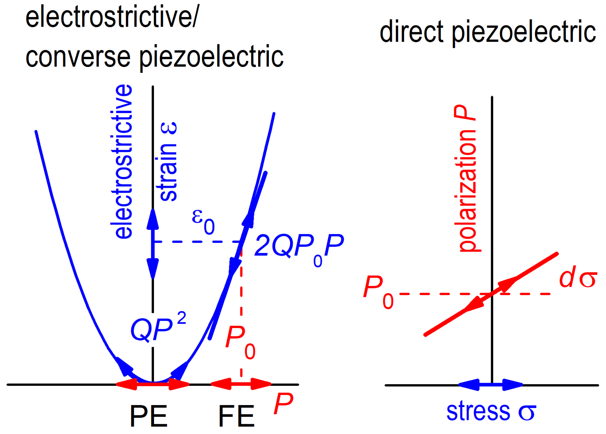
where $\epsilon$ and $\sigma$ are strain and stress, $s^0$ is the compliance at constant polarization P, coinciding with the total compliance in the PE phase with $P=0$, and the second term takes into account the fact that, in the FE state, the probing stress modulates the polarization, which in turn modulates the strain. This already makes clear that the additional softening in the FE state is due to a combination of direct and converse piezoelectric effects. The equilibrium spontaneous polarization $P\left(\sigma \right)$ under stress can be found by exploiting the fact that it minimizes the free energy $F=U-TS$. Actually, under the conditions of applied stress, the elastic Gibbs energy

$$G=F-\sigma \epsilon$$

(6)

[14] is minimized, since its differential is $dG=-SdT-\epsilon d\sigma +EdP$ with $\sigma$ rather than $\epsilon$ as independent variable, and $\epsilon$ is found from

$$\epsilon =-\frac{\partial G}{\partial \sigma }.$$

(7)

The description of the FE state is contained in the free energy $F\left(P,T\right)$, which generally is expanded in a series of even powers of P, according to the Landau theory of phase transitions. For deducing Equation (2) we do not need to specify the form of $F\left(P,T\right)$, but only that of the coupling $G_c\left(P,\sigma \right)$ between P and $\sigma$. The simplest form of such a coupling term, in a material with centrosymmetric (non piezoelectric) PE phase, is [15]

$$G_c\left(P,\sigma \right)=-Q\sigma P^2,$$

(8)

to be added to Equation (6), where Q is the electrostrictive coupling constant, and the electrostrictive strain is, according to Equation (7), $Q{P}^2$. A piezoelectric coupling $-g\sigma P$ cannot be introduced, because G must describe both the FE and PE states, and we are dealing with materials with a, generally cubic, PE state invariant under inversion, and a term $\propto \sigma P$ changes sign under inversion. The piezoelectric strain arises in the FE state with spontaneous polarization $P_0$, as shown in Figure 1. In fact, the electrostrictive strain, $Q{P}^2$, is quadratic in P in the PE state around $P=0$, but is almost linear with slope $2Q{P}_0$ in the FE state with spontaneous polarization $P_0$ and spontaneous strain ${\epsilon }_0$. This is at the basis of the converse piezoelectric effect, $d\epsilon /dE=$ $\left(d\epsilon /dP\right)\left(dP/dE\right)=$ d, whose coefficient is $d=2Q{P}_0\chi$, because $dP/dE=\chi$, the dielectric susceptibility.

The direct piezoelectric effect is, by definition, $dP/d\sigma =d$, and it is easy to verify that it is the same coefficient as for the converse effect. In fact, $P\left(\sigma \right)$ and its stress derivative can be found from the condition of minimum elastic Gibbs energy, Equations (6) and (8)

$$0=\frac{\partial G}{\partial P}=\frac{\partial F}{\partial P}-2\sigma QP,$$

which can be derivated with respect to $\sigma$ yielding

$$0=\frac{{\partial }^{2}F}{\partial P^2}\frac{dP}{d\sigma }-2QP-2\sigma Q\frac{dP}{d\sigma },$$

because F is a function of P only. In addition,

$$\frac{{\partial }^{2}F}{\partial P^2}={\chi }^{-1}$$

and the last term can be neglected because the probing stress $\sigma$ is small, so that we find

$$\frac{dP}{d\sigma }=2Q{P}_0\chi =d,$$

(9)

with the same coefficient as the converse effect.

We can now substitute our results for the FE state, $d\epsilon /dP=2Q{P}_0$ and $dP/d\sigma =2Q{P}_0\chi$ into Equation (5):

$$s\equiv s^0+4\chi Q^2{P}_0^2=s^0+d^2/\chi .$$

(10)

Finally, $ϵ=1+\chi ,$ so that in the FE state one generally has $1\ll \chi \simeq ϵ$ and Equations (2) and (10) coincide.

This result is general, since no hypothesis has been done on the form of $F\left(P\right)$, but it does not tell us what kind of temperature dependence we expect from $P_0$ and $\chi$, and hence d and $\Delta s^{\mathrm{piezo}}$; yet, it is useful to anticipate this temperature dependence, since the elastic measurement must be extended above and below $T_{\mathrm{C}}$, in order to recognize and subtract the non-ferroelectric contribution $s^0\equiv s^D$.

2.2. Temperature Dependence of the Piezoelectric Softening in the Simplest Case

The behaviour of $P_0,$ $\chi$ and d below the Curie temperature $T_{\mathrm{C}}$ can be predicted by specifying the free energy $F\left(P\right)$, which describes the FE state. The minimal form of $F\left(P\right)$ able to reproduce a FE transition is [15]

$$\begin{array}{ccc}\hfill F& =& \frac{\alpha }{2}{P}^2+\frac{\beta }{4}{P}^4\hfill \\ \hfill \alpha & =& {\alpha }_0\left(T-T_{\mathrm{C}}\right)\hfill \end{array}$$

(11)

where odd powers of P are excluded, because the minimum in the PE phase must be at $P=0$; the coefficient of the quadratic term becomes negative below $T_{\mathrm{C}}$, giving rise to minima at $P_0\ne 0$ in the FE phase. The condition for these minima is $0=\partial F/\partial P$, whose solution is

$$P_0^2={\alpha }_0\left(T_{\mathrm{C}}-T\right)/\beta .$$

(12)

The dielectric susceptibility $\chi$ is

$${\chi }^{-1}={\left.\frac{{\partial }^{2}F}{\partial P^2}\right|}_{P_0}=2{\alpha }_0\left(T_{\mathrm{C}}-T\right)$$

(13)

in the FE state and ${\alpha }_0\left(T_{\mathrm{C}}-T\right)$ in the PE state, that is the Curie-Weiss law. Substituting in Equation (10) we get

$$s=s^0+\frac{2Q^2}{\beta }$$

(14)

in the FE phase. Then, for a Curie-Weiss-like FE transition, the piezoelectric softening is simply constant, $\Delta s^{\mathrm{piezo}}=$ $2Q^2/\beta$, because the temperature dependencies of $P_0^2$ and $\chi$ cancel out exactly (Figure 2a). This s an idealized situation, and the various factors that influence the temperature dependence of the piezoelectric softening are illustrated in Figure 2b–d.

2.3. Anharmonic Stiffening and Electrostrictive Coefficients

The background compliance $s^0$ is not constant, but undergoes anharmonic stiffening on cooling. The result is an almost linear decrease of $s^0\left(T\right)$, at least down to 100 K, in the absence of other structural transitions. For example, the Young’s modulus $Y=s^{-1}$ of polycrystalline SrTiO${}_3$ increases of 2.9% per 100 K, while that of BaTiO${}_3$ of ≳$1.5\%$ per 100 K [10]. This effect can be estimated by extending the elastic measurement well above $T_{\mathrm{C}}$, in order to extrapolate $s^0\left(T\right)$ from a temperature region unaffected by the precursor FE fluctuations, where only the linear anharmonic stiffening is observed. In BaTiO${}_3$, the precursor fluctuations persist even 200 K above $T_{\mathrm{C}}$. Similarly, in systems with relaxor-like characteristics, $s^0\left(T\right)$ should be extrapolated from above the Burns temperature. Nevertheless, the anharmonic stiffening is a small effect, less important than other sources of uncertainty.

Also the electrostrictive coefficients Q are expected to increase slightly and linearly with temperature, since they also can be deduced by simple anharmonic models of inter-ionic potential [16]. Indeed, they are found to be little [17,18] or mildly [19] dependent on temperature, and composition in solid solutions, [18,20,21] so that, for simple FE transitions as described by Equation (11), one expects that the steplike softening below $T_{\mathrm{C}}$ remains nearly constant in a wide temperature range. Actually, one is not interested in the dependence of Q on T, because it contributes to that of $d\left(T\right)$ much less than $P_0$ and $ϵ$, and the use of Equation (2) does not require the separate knowledge of $P_0$ and Q.

2.4. Fluctuations and Thermoelastic Effect

Fluctuations are source of uncertainty, since they are not included in the treatment for deducing $\Delta s^{\mathrm{piezo}}$, and, though they affect also the piezoelectric and dielectric constants, there is no guarantee that s, $ϵ$ and d are equally affected, and therefore that Equation (2) is valid also in the presence of fluctuations. The effect of fluctuations is schematically shown in Figure 2c, together with that of thermoelastic relaxation [22]

$$\Delta s^{\mathrm{th}}=\frac{{\alpha }^{2}T}{C_{\sigma }},$$

(15)

where $\alpha$ is the coefficient of thermal expansion and $C_{\sigma }$ the specific heat. The thermoelastic effect occurs only in measurements where the sample vibration induces a inhomogeneous hydrostatic component of strain, as is the case of flexure. Since $\alpha$ is generally very peaked around $T_{\mathrm{C}}$, also $\Delta s^{\mathrm{th}}$ is peaked there. In BaTiO${}_3$, it can be estimated that $\Delta s^{\mathrm{th}}\simeq 0.1\Delta s^{\mathrm{piezo}}$ only very close to $T_{\mathrm{C}}$ and otherwise negligible. Even though a sizeable decay of $\Delta s^{\mathrm{piezo}}$ below $T_{\mathrm{C}}$ may be an intrinsic effect from a $F\left(P\right)$ more complicated than Equation (11) (see Section 2.6), the contribution of fluctuations is difficult or impossible to quantify, and it is better to not consider the temperature region close to $T_{\mathrm{C}}$.

2.5. Flexoelectric and Surface Effects

Other mechanisms that may induce polarization in the PE phase are the flexoelectric and surface effects [23], important in thin films, but generally neglected in ceramics. These effects are difficult to measure quantitatively, with experimental values of the flexoelectric coefficients sometimes exceeding the theoretical ones by two orders of magnitude [23,24]. Recently, it has been proposed that also the surface of ceramics may be polarized in the PE state, with ${\mathbf{P}}_s$ pointing outside the surface, so that the sample is overall unpoled, but under bending or inhomogeneous stress it exhibits enhanced effective flexoelectric coefficents [24]. The polarization would be due to flexoelectric effect from the inhomogeneous stress of the grains near the surface, which are less constrained perpendicularly to the surface down to several micrometers.

These effects, together with fluctuations, result in the formation of spontaneous polarization above $T_{\mathrm{C}}$ with null space average, so that they cannot be revealed with macroscopic measurements of the piezoelectric effect, but they contribute to the elastic and dielectric softenings. The elastic softening stands out of the weak linear anharmonic background (Figure 2b and Figure 4b), while the dielectric softening is certainly more difficult to separate from the Curie-Weiss rise of the permittivity toward $T_{\mathrm{C}}$. It cannot be excluded that Equation (2) partly holds also above $T_{\mathrm{C}}$, but the piezoelectric coefficient d in the PE state would be defined locally, with little practical value.

2.6. Additional Terms in the Expansion of $F\left(P\right)$ and Multiple Ferroelectric Transitions

In general, a faithful representation of the FE transition may require additional terms in the power expansion of $F\left(P\right)$, with respect to Equation (11). For example, a first order transition requires that $\beta <0$ and at least a positive term $\propto P^6$. A FE transition followed by other transitions where the spontaneous polarization ${\mathbf{P}}_0$ changes direction, as in BaTiO${}_3$, requires many more terms, fully expanded in terms of the components of the vector ${\mathbf{P}}_0$ in order to introduce the anisotropy. The explicit expressions for $\Delta s^{\mathrm{piezo}}$ in such cases may become very cumbersome and, in the few cases where they have been obtained, they have been analyzed numerically for selected sets of the parameters [20,21,25].

This is indeed the case of many FE perovskites of practical interest, for example with a morphotropic phase boundary between rhombohedraland tetragonal phases, as in PZT and PZT-based solid solutions, or with a sequence of FE transitions, as in BaTiO${}_3$ and BaTiO${}_3$-based solid solutions. The additional FE instabilities enhance the various susceptibilities, and this is exploited for improving the piezoelectric properties [26,27]. It is also possible to show in a simplified manner, that the compliance, and hence also the piezoelectric coefficients, is peaked at transitions where the spontaneous polarization changes direction, due to almost linear coupling between the transverse component of ${\mathbf{P}}_0$ and a shear strain [27,28]. Therefore, until the additional FE transitions are all describable by a same $F\left(\mathbf{P}\right)$ and the fluctuations and thermoelastic effects are not important, $\Delta s^{\mathrm{piezo}}$ will present additional peaks and anomalies, but Equation (2) should remain valid.

2.7. Additional Structural Transitions

Equation (2) is no more valid if other types of distortion modes are concomitantly present, in addition to the ferroelectric mode. The typical case in perovskites is an octahedral tilt mode, as in Na${}_{1/2}$Bi${}_{1/2}$TiO${}_3$ (NBT) or PZT with less than 50% Ti. The tilt mode mode is described by an additional order parameter $\varphi$, for example the angle of rotation of the octahedra. Then, the free energy F contains additional terms with even powers of $\varphi$, possible FE-tilt coupling terms containing both P and $\varphi$, and the coupling between $\varphi$ and stress $\sigma$ is exactly of the form (8) of the electrostrictive coupling, $\propto \sigma {\varphi }^2$ [29,30]. As a consequence, if the coupling between FE and tilt modes is weak, with two transitions well separated in temperature, the compliance will undergo two well separated softenings at the two transitions, and the previous treatment is still valid at the FE transition. It is impossible to distinguish which is the FE transition from the elastic measurement alone, but it is very easy from the dielectric susceptibility. In fact, the latter presents a huge peak of Curie-Weiss type at the FE transition, but only a small step at the tilt transition, if this occurs within the ferroelectric phase. This is due to the coupling between polarization and tilting, which, for symmetry reasons, to the lowest order is biquadratic [30], $\frac{k}{2}{P}^2{\varphi }^2$, and simply renormalises the $\frac{\alpha }{2}{P}^2$ term in the free energy (11) as $\frac{1}{2}\left(\alpha +k{\varphi }^2\right)P^2$ and the susceptibility in the FE phase, Equation (13), from $\chi =1/\left(2\alpha \right)$ to $1/2\left(\alpha +k{\varphi }^2\right)$. Below the tilt transition transition temperature $T_{\mathrm{T}}$, $\varphi$ passes from 0 to ${\varphi }_0\left(T\right)$ producing a step in $\chi ,$which is positive for cooperative ($k<0$) and negative for competitive tilt-polarization coupling, but very small compared to the FE peak.

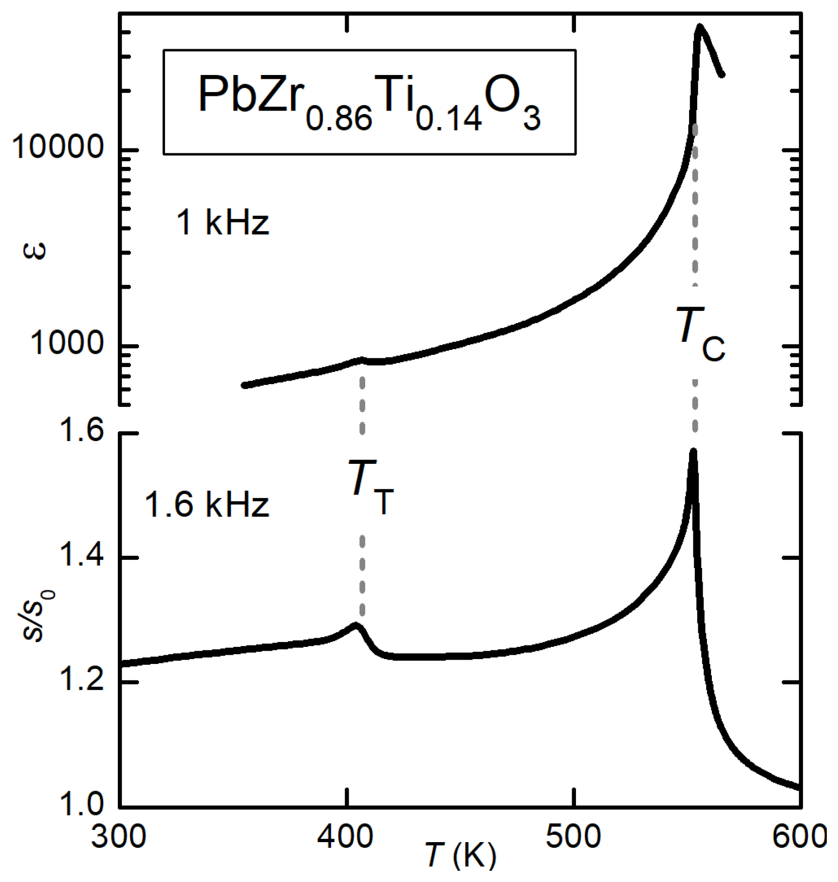
As an example, Figure 3 shows the compliance and dielectric susceptibility of PbZr${}_{0.86}$Ti${}_{0.14}$O${}_3$ [31], where the softening at $T_{\mathrm{T}}$ is smaller but of the same order of magnitude as that at $T_{\mathrm{C}}$, but the anomalies in the dielectric susceptibility (notice the logarithmic scale) leave no doubt on the different nature of the two transitions: polar ferroelectric at $T_{\mathrm{C}}$ and nonpolar antiferrodistortive at $T_{\mathrm{T}}$. In this case the softening below $T_{\mathrm{C}}$ should be purely piezoelectric down to $T_{\mathrm{T}}$.

In NBT and NBT-rich perovskites, instead, the tilt and polar modes are strongly coupled and act together at the structural transitions [32], so that there is no way of extracting the piezoelectric contribution from the softening [33].

2.8. Depolarization Field and Influence of the Measurement Frequency

Up to now we neglected the presence of the depolarization fields ${\mathbf{E}}^{\mathrm{dep}}$ created by the polarization charges at the domain walls and grain boundaries. Let us first consider a uniformly polarized (monodomain) sample, where ${\mathbf{E}}^{\mathrm{dep}}=-{ϵ}^{-1}·\mathbf{P}$. The application of an external probing stress $\sigma$ changes the polarization through the piezoelectric effect of $\delta \mathbf{P}=\mathbf{d}:\sigma$, which in turn changes the depolarization field by $\delta {\mathbf{E}}^{\mathrm{dep}}=-{ϵ}^{-1}·\mathbf{d}:\sigma$; finally, through the converse piezoelectric effect, an additional strain is generated: $\delta \epsilon ={\mathbf{d}}^{+}·$ $\delta {\mathbf{E}}^{\mathrm{dep}}=$ $-{\mathbf{d}}^{+}·{ϵ}^{-1}·\mathbf{d}:\sigma$. This corresponds to a stiffening of the compliance $\Delta s^{\mathrm{stiff}}=$ $\delta \epsilon /\sigma =$ $-{\mathbf{d}}^{+}·{ϵ}^{-1}·\mathbf{d}$, known as piezoelectric stiffening [34], and exactly cancelling the piezoelectric softening, $\Delta s^{\mathrm{stiff}}=$ $-\Delta s^{\mathrm{piezo}}$, in the case of uniform polarization [11].

On the other hand, if the sample is unpoled and the vibration stress is uniform over a length scale including several domains, $\overline{\delta \mathbf{P}}=\overline{\mathbf{d}}:\sigma \simeq 0$, because $\overline{\mathbf{d}}\simeq 0$. This condition holds for forced or resonant vibrations of macroscopic samples, with sizes of several millimeters and more, but for ultrasound experiments, the wavelength must be sufficiently long to include several domains, otherwise, partial piezoelectric stiffening may occur, which reduces $\Delta s^{\mathrm{piezo}}$. An extreme case are the Brillouin scattering experiments, where the probe acoustic waves at ∼50 GHz have $\lambda \lesssim 0.1$ $\mathsf{\mu }$m. In this case, the wavelength probes regions within single domains with uniform $\mathbf{P}$, and $\Delta s^{\mathrm{piezo}}$ is considerably or totally cancelled by $\Delta s^{\mathrm{stiff}}$. A comparison between the compliance of PbZr${}_{0.55}$Ti${}_{0.45}$O${}_3$ measured on a resonating bar at kHz and with Brillouin scattering [11], shows that in the latter experiment only a small peak at $T_{\mathrm{C}}$, due to fluctuations, is present, but no piezoelectric softening; instead, the tilt transition at $T_{\mathrm{T}}\ll T_{\mathrm{C}}$ produces a step in both measurements, because it does not involve changes in polarization and hence no piezoelectric softening and stiffening.

In addition to the averaging over several domains in the unpoled state, a further reduction of the depolarization field may be effected by the free charges from ionized defects, which neutralize the polarization charges at the DW.

2.9. Extrinsic Domain Wall Contributions

All the above formulas take into account the intrinsic piezoelectric effect, without movement of the domain walls (DW); yet, the DW motion may considerably enhance the magnitude of the measured piezoelectric coefficients [12,35], especially for high stress levels and low frequencies. The relationship (1) between dielectric, elastic and piezoelectric coefficients does not necessarily hold also for effective coefficients, that include the effect of the DW motion, even if this is within the limit of linear response. For simplicity, let us drop the tensor notation and consider appropriate components, e.g., the longitudinal components for an extensional or flexural vibration of a bar. Then Equation (1) can be written as

$$d^2=\Delta \chi \Delta s,$$

(16)

where the superscript in $\Delta s^{\mathrm{piezo}}$ is dropped and it is put in evidence that only the part $\Delta \chi$ of $\chi$ arising from the FE transition, Equation (13), must be considered (in practice for most ferroelectrics it is $\chi =$ ${\chi }_{\infty }+\Delta \chi \cong$ $\Delta \chi$). A similar relationship holds for the contributions from defects with elastic and dielectric dipoles, causing dielectric, anelastic and piezoelectric relaxations of amplitudes $\delta \chi$, $\delta s$ and $\delta d$ [27,36,37]:

$${\left(\delta d\right)}^2=\delta \chi \delta s.$$

(17)

However, even assuming that the linear contribution from DW motion satisfies this relation, the total effective coefficients, $\tilde{\chi }=\Delta \chi +\delta \chi$, $\tilde{s}=\Delta s+\delta s$ and $\tilde{d}=d+\delta d$, do not necessarily obey ${\tilde{d}}^2=\tilde{\chi }\tilde{s}$. It can be shown that this is true only if $\delta s/\Delta s=\delta \chi /\Delta \chi$, but there is no apparent reason for such a relationship to be true in general.

Therefore, Equation (1) strictly holds only for the intrinsic piezoelectric coefficients, without contributions from DW motion, and it seems safe to limit the analysis of the piezoelectric activity in terms of elastic softening only to measurements with low stress amplitude and linear response, where the DW motion is reversible and minimal. At large stresses, where the elastic response is nonlinear, one probes the irreversible motion of DW, with pinning and unpinning processes, corresponding to the regions of the hysteresis loops with steep slopes. In these regions, the piezoelectric coefficients are anyway ill-defined.

2.10. Polycrystalline Average of Unpoled Ceramic: A Well Defined State

The elastic moduli of ceramic samples are angular averages of the single crystal material constants, and therefore Equation (2) must be averaged over all domain orientations. The great advantage of using unpoled ceramics is that the orientations are really random, unless a particular texture exists, and therefore the orientation averages are simple. Instead, the orientational averages for poled samples are more complicated (see e.g., Ref. [38]) and provide theoretical bounds to the maximum polarization, but the actual degree of poling of a sample depends on several factors: (i) the degree of non$-{180}^{\circ }$ DW motion and switching, which generally is well below 100%, due to internal mechanical constraints; (ii) DW pinning; (iii) non-uniform internal fields, due to porosity, microstructure and defects; (iv) insufficient poling field, due to instrumental limitations, and the geometry and resistance to fracture of the sample. As a consequence, it is possible that the degree of poling is considerably below the theoretical maximum, but it is difficult or impossible to establish how much.

It can be concluded that the unpoled state of an untextured ceramic is much better defined than its poled state, and therefore better suited to study the intrinsic behaviour of the material. The orientational averages of $\Delta s^{\mathrm{piezo}}$ in terms of the single crystal material constants for randomly oriented domains are easy to calculate, and the results for tetragonal, orthorhombic and rhombohedral symmetries are [10]:

$$\overline{\Delta s^{\mathrm{piezo},\mathrm{T}}}=\frac{8d_{31}^2+4d_{31}{d}_{33}+3d_{33}^2}{15{ϵ}_{33}}+\frac{2d_{15}^2}{15{ϵ}_{11}}$$

(18)

$$\begin{array}{cc}\hfill \overline{\Delta s^{\mathrm{piezo},\mathrm{O}}}& =\frac{3d_{31}^2+3d_{32}^2+3d_{33}^2}{15{ϵ}_{33}}+\hfill \\ & \frac{2d_{31}\left(d_{32}+d_{33}\right)+2d_{32}{d}_{33}}{15{ϵ}_{33}}+\frac{d_{15}^2}{15{ϵ}_{11}}+\frac{d_{24}^2}{15{ϵ}_{22}}\hfill \end{array}$$

(19)

$$\overline{\Delta s^{\mathrm{piezo},\mathrm{R}}}=\frac{8d_{31}^2+4d_{31}{d}_{33}+3d_{33}^2}{15{ϵ}_{33}}+\frac{\left(2d_{15}^2+4d_{22}^2\right)}{15{ϵ}_{11}},$$

(20)

where the Voigt index notation is adopted.

Unfortunately, the single crystal materials constants are generally unknown for most ferroelectrics, and, in order to use the above formulas for quantitative comparisons, one must express the single crystal $d_{ij}$ and ${ϵ}_{ij}$ coefficients in terms of the effective $d_{ij}^{\ast }$ and ${ϵ}_{ij}^{\ast }$ measured on ceramics. This is done, for example, in Ref. [38], and we report below the result for tetragonal symmetry, assuming full poling and adopting the original notation $\overline{d^{\ast }}$ instead of $d^{\ast }$

$$\begin{array}{ccc}\hfill d_{33}& =& 2.316\overline{d_{33}^{\ast }}-1.113\left(\overline{d_{31}^{\ast }}+\overline{d_{15}^{\ast }}\right)\hfill \end{array}$$

(21)

$$\begin{array}{ccc}\hfill d_{31}& =& 1.760\overline{d_{31}^{\ast }}-0.5565\left(\overline{d_{33}^{\ast }}-d_{15}^{\ast }\right)\hfill \end{array}$$

(22)

$$\begin{array}{ccc}\hfill d_{15}& =& 2.316\overline{d_{15}^{\ast }}-1.113\left(\overline{d_{33}^{\ast }}-\overline{d_{31}^{\ast }}\right)\hfill \end{array}$$

(23)

$$\begin{array}{ccc}\hfill {ϵ}_{11}& =& 1.222\overline{{ϵ}_{11}^{\ast }}-0.261\overline{{ϵ}_{33}^{\ast }}\hfill \end{array}$$

(24)

$$\begin{array}{ccc}\hfill {ϵ}_{33}& =& 1.482\overline{{ϵ}_{33}^{\ast }}-0.261\overline{{ϵ}_{11}^{\ast }}\hfill \end{array}$$

(25)

2.11. Experimental Verification and Porosity

Up to now there is only one experimental verification of the validity of Equation (2), based on ceramic BaTiO${}_3$ [10]. The reason it is difficult to carry out a quantitative verification is connected with the difficulty of finding a material with reliably known piezoelectric and dielectric tensors. In addition, the technique available in our laboratory requires samples shaped as bars longer than 2 cm (but DMA, RUS and ultrasonic experiments can be performed on much smaller samples). The ceramic samples must also possess the same physical properties as the crystals, apart from the unavoidable porosity, and this excludes the usual piezoelectric materials, whose properties are heavily dependent on composition, additives and preparation protocols. The material of choice is therefore pure BaTiO${}_3$, though it has the complication of strong FE fluctuations extending 200 K above $T_{\mathrm{C}}$, and two additional FE transitions below $T_{\mathrm{C}}$.

The comparison between $\Delta s^{\mathrm{piezo}}$, Equation (18), deduced from the Young’s modulus of ceramic bars of BaTiO${}_3$ measured at kHz and the literature data for $d_{ij}$ and ${ϵ}_{ij}$ is described and discussed in detail in Ref. [10], and here only a brief account is given. A major problem in comparing materials constants measured on ceramics with single crystal data is porosity, whose effect can be estimated only with great uncertainty. In Figure 4a the compliances of three different samples from different laboratories (sample 1 measured in Ref. [39] and samples 2 and 3 in Ref. [10]) differ of factors up to 4, even though the porosities from the Archimedes method differ at most of a factor of 3 and the dependence of s on porosity is definitely nonlinear. In fact, the shape of the pores has a major influence and is difficult to assess. Nonetheless, by rescaling in Figure 4b the softer $s\left(T\right)$ curves of the more porous samples on the stiffer curve of sample 1 well above $T_{\mathrm{C}}$, one finds a fair agreement between all the curves also below $T_{\mathrm{C}}$. This encourages one to use the data of porous ceramics even to evaluate the material intrinsic piezoelectric properties, based on the effect of porosity in the PE phase. Notice that, if one wants to deduce piezoelectric coefficients from the elastic softening and permittivity measured on porous ceramics, also the permittivity must be renormalised for taking into account the porosity, but the effects of porosity on the elastic and dielectric responses may be different, so that there is no guarantee that the same rescaling factor applies to s and $ϵ$. For reducing the uncertainty one should reduce the porosity.

The $s^0\left(T\right)$ has been extrapolated from >800 K, since already below that temperature its linear dependence is obscured by the rising precursor softening from the FE fluctuations and polarization induced by flexoelectric and surface effects. After subtraction of $s^0\left(T\right)$ one gets $\Delta s^{\mathrm{piezo}}\left(T\right)$ (Figure 4c), which can be compared with the averaged expression, Equation (18), where the single crystal $d_{ij}$ and ${ϵ}_{ij}$ are inserted. Even for BaTiO${}_3$, there are no accepted values for these parameters, and the two curves are calculated using values measured on a set of single crystals [40], and values obtained from a Landau free energy, that reproduce many experimental data on BaTiO${}_3$ [41].

The agreement between the measured and calculated $\Delta s^{\mathrm{piezo}}$ is good only in the plateau of $s\left(T\right)$ below $T_{\mathrm{C}}$ and well above the transition temperature $T_{\mathrm{OT}}$ between the FE tetragonal (T) and FE orthorhombic (O) phases. In this temperature region the fluctuations of the polarization should be minimal, and indeed both the calculated curves cross the experimental ones there. Notice that longitudinal fluctuations of the polarization are present near and above $T_{\mathrm{C}}$, but transverse fluctuations are expected above $T_{\mathrm{OT}}$, where they are associated with the change of direction of the spontaneous polarization (Figure 4d).

As discussed in Section 2.6, $\Delta s^{\mathrm{piezo}}$ should include also the peaked softenings at $T_{\mathrm{OT}}$ and $T_{\mathrm{RO}}$, and it is not clear if the fluctuations together with surface and flexoelectric effects may explain the difference between the measured and calculated curves, away from the plateau of $s\left(T\right)$. It is true that also the calculated curves do not agree with each other, but there seems to be a systematic difference between the temperature dependencies of the measured and calculated piezoelectric softenings. The motion of domain walls may also be responsible for such deviations, but the analysis of the $s\left(T\right)$ and elastic energy loss curves measured at different frequencies [42] suggests that the contribution of DW relaxation is negligible, at least in curves 2 and 3.

It can be concluded that, at least in a limited temperature region below $T_{\mathrm{C}}$ where complications from fluctuations and multiple FE transitions are excluded, there is quantitative agreement between the piezoelectric softening measured on unpoled ceramic BaTiO${}_3$ and that calculated from the known piezoelectric and dielectric tensors.

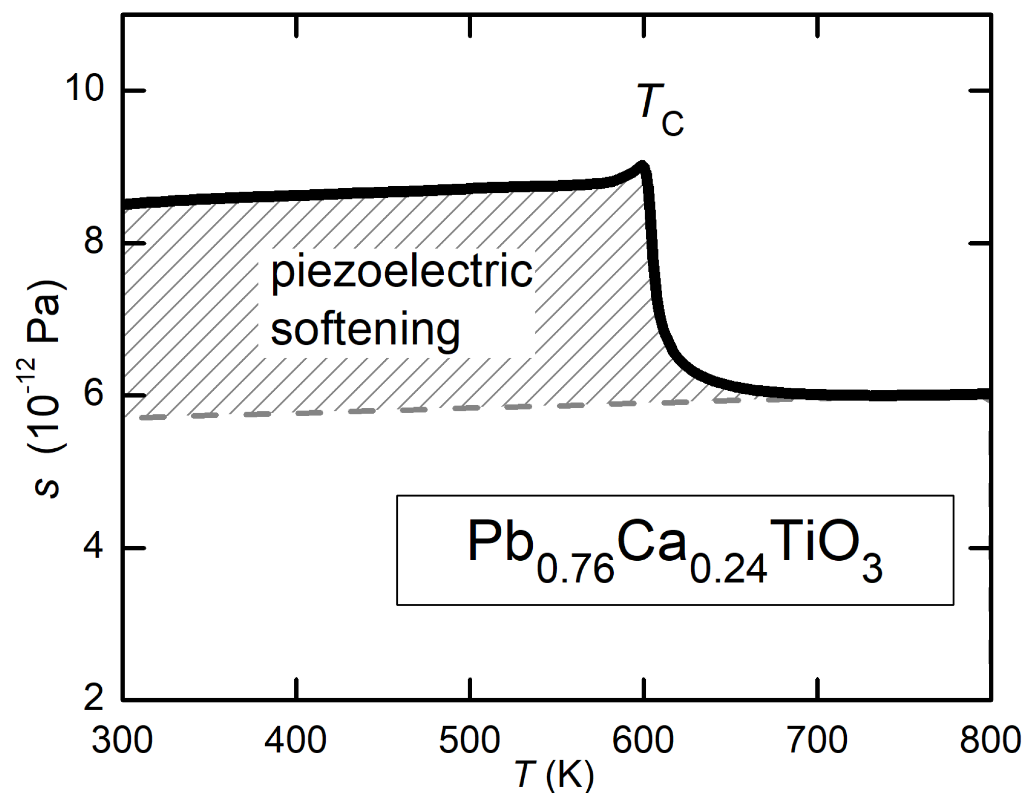
In ferroelectrics with a single or at least more isolated FE transition, the situation should be more clear. For example, PbTiO${}_3$ doped with Ca has only one transitions from C-PE to T-FE, and no tendency to octahedral tilting. Indeed, preliminary measurements (Figure 5) of the Young’s modulus at kHz show a situation very close to the simple case in Figure 2c. Further piezoelectric and dielectric measurements are in progress [43] on samples from the same material, in order to make a quantitative comparison between the softening of Figure 5 and Equations (18) with (21)–(25).

2.12. Usefulness of the Elastic Assessment of the Potential Piezoelectric Properties of Unpoled Samples

The use of Equation (2), and hence Equations (18)–(20), to extract the intrinsic piezoelectric coefficients $d_{ij}$ seems particularly promising in combination with Resonant Ultrasound Spectroscopy (RUS) experiments on unpoled ceramics, from which the full tensors $s_{ij}^E$ in the FE state and $s_{ij}^0=s_{ij}^D$ in the PE state can be extracted. This type of experiments has been done for extracting the elastic tensor $s_{ij}^E$ of unpoled PZT-4 in the FE state [44], and by piezoelectrically exciting a poled PZT-8 ceramic sample [9], so obtaining the full piezoelectric and elastic tensors in the FE state. The latter method is certainly a considerable improvement with respect to the traditional methods requiring sets of different samples, but still the piezoelectric coefficients depend on the degree of poling. Measuring unpoled samples over the full FE and PE temperature range would avoid also this source of uncertainty. The analysis of the full resonance spectrum of a poled ceramic disc [8] is similar to the piezoelectrically excited RUS [9], though with a larger sample.

At present, few laboratories measure the full elastic tensor with the RUS technique, and the more common acoustic measurements adopt forced (Dynamic Mechanical Analyzer = DMA, torsional pendulum) or resonant vibrations of bars, or ultrasonic propagation in pellets. While the ultrasonic experiments allow longitudinal and transverse waves to be excited, the other methods provide only one type of modulus, Young’s or torsional. In these cases it is impossible to extract the three or more components of $d_{ij}$, but the piezoelectric softening can still provide useful information. This is particularly true when studying new materials, or the effect of new types of doping or preparation protocols. In these cases, it is possible that varying some composition or preparation parameter, renders the poling of the sample less effective or impossible, for example due to increased conductivity or coercive field. A comparison of the piezoelectric softenings of the series of unpoled samples would provide a reliable indication of the potential piezoelectric response, that each sample would have if it would be fully poled, without the need for actually poling it, and therefore before optimizing composition and process in order to make poling easier.

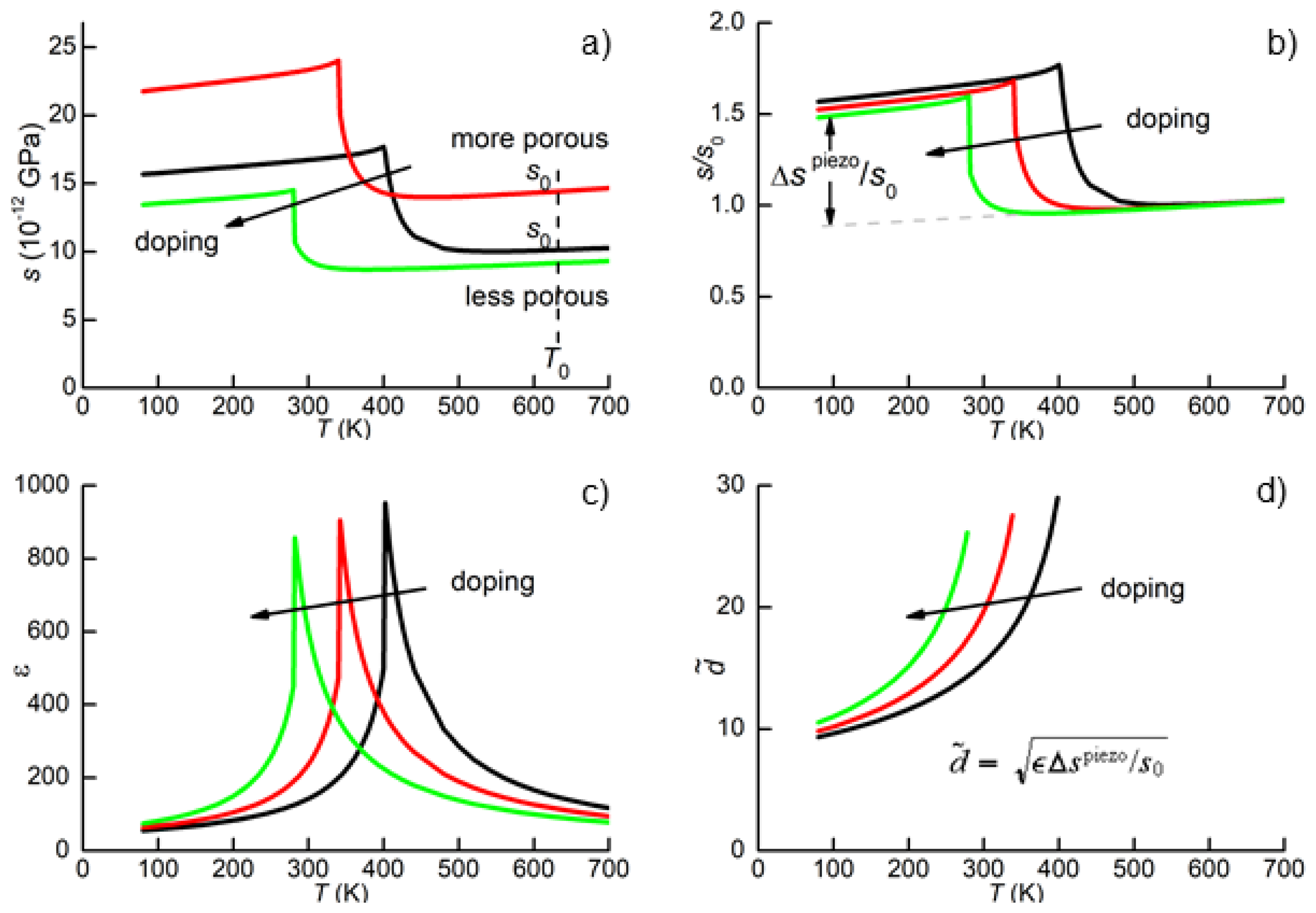
A possible course of action in similar instances is illustrated in Figure 6. Figure 6a shows three hypothetical compliance curves obtained by varying a material parameter, for example doping. Increasing doping lowers $T_{\mathrm{C}}$ and changes the amplitude of $\Delta s^{\mathrm{piezo}}$, but the main differences between the magnitude of the compliances are due to different porosities. Therefore, in Figure 6b the curves are normalized in order to overlap in the PE phase, where it is assumed that doping has little effect on the elastic properties. This is done by choosing a temperature $T_0$ well above $T_{\mathrm{C}}$, where $s^0\left(T\right)$ increases linearly, due to anharmonic effects, as explained in Section 2.3. Then, each curve is normalized by $s_0=s^0\left(T_0\right)$ (Figure 6b). In this manner, the comparison between different $\Delta s^{\mathrm{piezo}}$ is not or little affected by porosity. The validity of this procedure is confirmed by tests on BaTiO${}_3$ (Figure 4a,b). The anharmonic stiffening of $s^0\left(T\right)$ is generally linear with very good approximation down to 100 K, so that it is easy to extrapolate it in FE phase and obtain $\Delta s^{\mathrm{piezo}}$. According to Equation (2) or (16), a measure of the piezoelectric response is provided by

$$\tilde{d}=\sqrt{ϵ\Delta s^{\mathrm{piezo}}/s_0}$$

(26)

It is adimensional, because one uses the normalized $\Delta s^{\mathrm{piezo}}$, in order to eliminate the influence of different porosities, but one may as well normalize the $s\left(T\right)$ curves to that with lower $s_0$, presumably from the denser sample: if $s_n$ is $s_0$ of the $n-$th curve, than one extracts its $\Delta s^{\mathrm{piezo}}$ from $\tilde{s}\left(T\right)=$ $s\left(T\right)\times \left(s_0/s_n\right)$ and calculates $\tilde{d}=\sqrt{ϵ\Delta {\tilde{s}}^{\mathrm{piezo}}}$ with the correct dimensions. The point is that, in this context, the absolute value of $\tilde{d}$ is of little interest, since it does not correspond to any $d_{ij}^{\ast }$ or $d_{ij}$, but to a combination of them; what is important is the evolution of $\tilde{d}$, measured in the same manner for the whole series of samples, with changing doping or the process parameters.

Also the dielectric permittivity is influenced by porosity, but in opposite manner with respect to the compliance, being reduced. If $ϵ$ were reduced by the same factor as s, the effect of porosity would be automatically cancelled in $\Delta s^{\mathrm{piezo}}$, without any correction. Unfortunately, this is not necessarily true (see e.g., Equation (18) in [45]), so that a quantitative analysis would require the use of Equation (26), where also $ϵ$ is rescaled in order to cancel the effect of porosity. This is not as easy as for the compliance, since the FE instability causes a Curie-Weiss peak in $ϵ$, rather than a step below $T_{\mathrm{C}}$, whose contribution extends to the PE phase. Therefore, rather than simply renormalising $ϵ$ with its value at some $T_0>$ $T_{\mathrm{C}}$, one should extract the high frequency limits ${ϵ}_{\infty }$ and use $ϵ/{ϵ}_{\infty }$ in Equation (26). For qualitative purposes, it seems appropriate to use $\tilde{d}$ or simply d, and use the variation from sample to sample in $s_0$ as an indication of the uncertainty introduced by changes in porosity.

Figure 6c shows the permittivity curves $ϵ\left(T\right)$, necessary to obtain $\tilde{d}\left(T\right)$. Only the part below $T_{\mathrm{C}}$ is useful, and, in case of high conductivity, it is convenient to use high enough a frequency, e.g., 1 MHz, to minimize the lossy conductivity contribution. The final result of this example in Figure 6d shows that doping decreases $T_{\mathrm{C}}$, but the piezoelectric response of the material is even increased, thanks to the increase of $ϵ$ with lower $T_{\mathrm{C}}$. This type of information is obtained without poling the sample, and calculating an effective $\tilde{d}$ according to Equation (26). The conclusion is valid even if doping introduces free carriers or strong DW pinning, which make actual poling impossible. Yet, one knows that the particular type of doping improves the intrinsic piezoelectric properties, and further material engineering can be attempted, in order to make poling easier.

Figure 7 presents another hypothetical instance, where doping transforms the FE transition into charge/orbital order, similarly to the manganite or nickelate perovskites. Below the onset of these types of transitions, a stiffening rather than softening is observed [46,47], so that it is easy to see by simple inspection that the FE transition is suppressed by doping.

2.13. Piezoelectric Softening Versus Electromechanical Coupling Factor

The knowledge of $s^D\equiv s^0$ and $s^E=s^D+\Delta s^{\mathrm{piezo}}$, see Equation (4), suggests another manner of exploiting the piezoelectric softening, defining the quantity $\tilde{k}$ as

$${\tilde{k}}^2=\Delta s^{\mathrm{piezo}}/s^E.$$

(27)

This is formally identical to the electromechanical coupling factor k, which is also of practical interest. The difference between k and $\tilde{k}$ is that the latter is measured on an unpoled ceramic, and therefore it should be an average of the three $k_{ij}^{\ast }$. An analysis in order to deduce expressions of $\tilde{k}$ in terms of $k_{ij}^{\ast }$ is not yet done, but it seems promising to interpret the piezoelectric softening in terms of electromechanical coupling, because it does not require the knowledge of the dielectric tensor. Following the discussion on the piezoelectric coefficients, the electromechanical coupling defined by Equation (27), measured on an unpoled ceramic, should provide an average of the $k_{ij}^{\ast }$, that the ceramic would have when fully poled. In this case, porosity would be much less problematic than when using Equation (2) to deduce intrinsic $d_{ij}$, since there is no need for knowing the compliance of the fully dense material: one simply measures the effective electromechanical coupling of the porous material under study.

3. Materials and Methods

The compliance curves shown here are all defined as $s\left(T\right)=1/E\left(T\right)$, where E is the Young’s modulus of ceramic bars 25–40 mm long, 4–5 mm wide and 0.6–1.2 mm thick. The dynamic Young’s modulus is measured by suspending the bars on thin thermocouple wires in vacuum or <0.2 mbar He exchange gas, electrostatically exciting their flexural resonant modes. Up to the first three odd modes can be probed during a same temperature scan, with frequencies in the ratios 1:5.4:13.3, with a fundamental resonance frequency 1–3 kHz, depending on the sample size and material. The vibration is detected including the same exciting electrode in a resonant circuit at ∼ 13 MHz, whose frequency is modulated bu the change of sample/electrode capacitance. The method is described in Ref. [48]. The Dynamic Mechanical Analyzer is another technique for obtaining the same dynamic modulus, though with forced vibrations at lower frequencies and higher amplitudes [49].

The samples were cut from ceramic bars prepared by standard solid state reaction, as described in Ref. [31] for PZT, Ref. [42] for BaTiO${}_3$, while the powders for PCT were prepared with a sol-gel process [50]. The porosities in Figure 4a were estimated as $p=1-\rho /{\rho }_{\mathrm{th}}$, with ${\rho }_{\mathrm{th}}=6.02$ g/cm${}^3$ and $\rho$ was measured with the Archimedes method. The porosity of sample 3 was probably underestimated, judging from the long equilibration time for measuring its weight in water [10]. The higher porosity of sample 3 and presumably its conformation more similar to fissures explains the considerably reduced Young’s modulus.

4. Conclusions

Below the paraelectric to ferroelectric transition, a material undergoes an elastic softening of piezoelectric origin. The relationship, Equation (1), between piezoelectric, elastic and dielectric coefficients $d_{ij}$, ${ϵ}_{ij}$ and $s_{ij}$ is contained in the standard thermodynamic theory of ferroelectricity, and it is demonstrated here in a intuitive manner. Though this relationship has never been exploited for practical purposes, it offers an alternative method for evaluating the intrinsic piezoelectric response of a ferroelectric material. The advantage over the traditional methods is that it can be used with unpoled ceramics, where it provides a measure of the intrinsic piezoelectric response, that a material would have after full poling, without poling it. Not only this allows one to get rid of the uncertainties connected with the actual level of poling of a sample, but also to probe the piezoelectric activity of samples which cannot be poled at all, for example due to excessive coercive field or conductivity.

In combination with dielectric permittivity and Resonant Ultrasound Spectroscopy experiments, where the full elastic tensor can be extracted, it is in principle possible to obtain both the elastic and piezoelectric tensors from a single measurement spanning the FE and PE states. With more traditional measurements of the Young’s modulus or torsional modulus at acoustic and subacoustic frequencies, it is not possible to separate all the components of the piezoelectric tensor, but to evaluate an angular average of them. The piezoelectric softening can also be evaluated from ultrasonic experiments, provided that the wave length probes several FE domains, so that any change induced in the depolarization field averages to zero.