Fully Kinetic Simulation of Ion-Temperature-Gradient Instabilities in Tokamaks

Abstract

The feasibility of using full ion kinetics, instead of gyrokinetics, in simulating low-frequency Ion-Temperature-Gradient (ITG) instabilities in tokamaks has recently been demonstrated. The present work extends the full ion kinetics to the nonlinear regime and investigates the nonlinear saturation of a single-n ITG instability due to the $E\times B$ trapping mechanism (n is the toroidal mode number). The saturation amplitude predicted by the $E\times B$ trapping theory is found to agree with the saturation level observed in the simulation. In extending to the nonlinear regime, we developed a toroidal Boris full orbit integrator, which proved to be accurate in capturing both the short-time scale cyclotron motion and long time scale drift motion, with good kinetic energy conservation and toroidal angular momentum conservation in tokamak equilibrium magnetic fields. This work also extends the previous work from analytic circular magnetic equilibria to general numerical magnetic equilibria, enabling simulation of realistic equilibria reconstructed from tokamak experiments.

1. Introduction

Ion temperature gradients in tokamaks provide free energy to micro-instabilities called Ion-Temperature-Gradient (ITG) instabilities [1]. The nonlinear development of these instabilities, i.e., ITG turbulence, is believed to play an important role in regulating particle and heat transport in tokamaks [2,3,4]. There are numerous papers devoted to the gyrokinetic simulation of ITG turbulence, which employ gyrokinetic theory to decouple the high-frequency gyro-motion of ions from the low-frequency ITG modes [5,6,7,8,9,10]. However, gyrokinetics rely on ordering assumptions in deriving the gyrokinetic equation. One of these ordering assumptions, ${\rho }_i/L_n\ll 1$, becomes questionable in tokamak edge with steep density profile, where ${\rho }_i$ is the gyro-radius of ions and $L_n$ is the scale length of density profile. For this reason, tokamak edge gyrokinetic codes, e.g., XGC [11,12], are usually limited in the regime where the pedestal width is much greater than the ion gyro-radius. Fully kinetic ion models [13,14,15,16,17,18], which retain the ion gyro-motion, avoid these problematic ordering assumptions (although involving more computations in simulations). Low-frequency full kinetics have already been demonstrated in slab geometry [19], successfully benchmarked against gyrokinetics for the slab ITG [20], and extended to toroidal ITG instabilities by Sturdevant et al. [21].

The present work extend that of Ref. [21] to the nonlinear regime and investigates the nonlinear saturation of a single-n ITG instability due to the $E\times B$ trapping mechanism (n is the toroidal mode number). The saturation amplitude predicted by the $E\times B$ trapping theory is found to agree with the saturation level observed in the simulation. In extending to the nonlinear regime, we developed a toroidal Boris full orbit integrator, which proved to be accurate in capturing both the short-time scale cyclotron motion and long time scale drift motion, with good kinetic energy conservation and toroidal angular momentum conservation in tokamak equilibrium magnetic fields. This work also extends the previous work from analytic circular magnetic equilibria to general numerical magnetic equilibria, enabling simulation of realistic equilibria reconstructed from tokamak experiments.

To verify the new numerical implementation of the orbit integrator and magnetic configuration, the linear electrostatic ITG frequency and growth rate are compared with the fully kinetic results of Ref. [21] and gyrokinetic results of Ref. [22]. Good agreement is found for both cases. Our simulation adopts the $\delta f$ particle-in-cell (PIC) method.

The remainder of the paper is organized as follows. Section 2 discusses the fully kinetic ion model for simulating ITG instabilities. The implicit $\delta f$ PIC method and the full orbit integrator are briefly discussed in Section 3. Section 4 discusses how magnetic configuration and magnetic coordinates are handled in our numerical model. Section 5 gives the linear and nonlinear results of ITG instabilities, along with a benchmark against the fully kinetic results of Ref. [21] and gyrokinetic results of Ref. [22] in the linear regime. A brief summary is given in Section 6.

2. Fully Kinetic Ion Model of ITG Instabilities

The fully kinetic ion model for ITG instabilities is described in Ref. [21]. The following is a summary of the model. The ion Vlasov equation is written

$$\frac{d{f}_i}{dt}\equiv \frac{\partial f_i}{\partial t}+\mathbf{v}·\frac{\partial f_i}{\partial \mathbf{x}}+\frac{q_i}{m_i}(\mathbf{E}+\mathbf{v}\times \mathbf{B})·\frac{\partial f_i}{\partial \mathbf{v}}=0,$$

(1)

where $f_i(\mathbf{x},\mathbf{v})$ is the ion distribution function, $\mathbf{x}$ and $\mathbf{v}$ are ion position and velocity respectively, $\mathbf{E}$ and $\mathbf{B}$ are the electric field and magnetic field respectively, $q_i$ and $m_i$ are the charge and mass of ions respectively. We write $f_i$ as an equilibrium part plus a perturbation, i.e., $f_i=f_{i0}+\delta f_i$, then Equation (1) is written as

$$\frac{d\delta f_i}{dt}=-\frac{q_i}{m_i}(\delta \mathbf{E}+\mathbf{v}\times \delta \mathbf{B})·\frac{\partial f_{i0}}{\partial \mathbf{v}},$$

(2)

where $\delta \mathbf{E}$ and $\delta \mathbf{B}$ are the perturbed part of the electric field and magnetic field, respectively.

To model ITG instabilities, the equilibrium part of ion distribution function $f_{i0}$ is chosen as [21]

$$f_{i0}(R_r,v)=n_{i0}\left(R_r\right){\left(\frac{m_i}{2\pi T_{i0}\left(R_r\right)}\right)}^{3/2}exp\left[-\frac{m_i{v}^2}{2T_{i0}\left(R_r\right)}\right],$$

(3)

where $n_{i0}$ and $T_{i0}$ are ion number density and temperature, which depend on a radial variable $R_r$ given by

$$R_r=r+\frac{m_i}{q_i}\frac{\mathbf{v}\times \mathbf{b}}{B_0}·\nabla r,$$

(4)

where r is the minor radius of magnetic surfaces and $\mathbf{b}={\mathbf{B}}_0/B_0$ is the unit vector along the equilibrium magnetic field ${\mathbf{B}}_0$. The variable $R_r$ is a radial coordinate of the ion guiding-center and thus an approximate constant of motion in the weakly inhomogeneous tokamak magnetic field with ${\rho }_i/L_B\ll 1$, where $L_B$ is the scale length of ${\mathbf{B}}_0$. Since arbitrary functions of the constants of motion are solutions to the kinetic equation, the distribution function given by Equation (3) is approximately an equilibrium solution to the kinetic Equation (1). Using this form of equilibrium distribution, the kinetic Equation (2) for the perturbed part of the distribution is written as

$$\begin{array}{ccc}\frac{d\delta f_i}{dt}\hfill & =\hfill & \frac{q_i}{T_i}{f}_{i0}\delta \mathbf{E}·\mathbf{v}+\left[{\kappa }_{n_i}+\left(\frac{m{v}^2}{2T_i}-\frac{3}{2}\right){\kappa }_{T_i}\right]f_{i0}\frac{(\delta \mathbf{E}\times \mathbf{b})·\nabla r}{B_0}\hfill \\ & -\hfill & \left[{\kappa }_{n_i}+\left(\frac{m{v}^2}{2T_i}-\frac{3}{2}\right){\kappa }_{T_i}\right]f_{i0}(\mathbf{v}\times \delta \mathbf{B})·\frac{\nabla r\times \mathbf{b}}{B_0},\hfill \end{array}$$

(5)

where ${\kappa }_{n_i}=-n_{i0}^{-1}\partial n_{i0}/\partial R_r$ and ${\kappa }_{T_i}=-T_{i0}^{-1}\partial T_{i0}/\partial R_r$ are the radial gradients of ion density and temperature, respectively.

The equilibrium distribution function (3) does not include neoclassical effects and imposes a constraint similar to that of gyrokinetic models. The purpose of adopting this distribution function is to reproduce the gyrokinetic ITG instabilities using the fully kinetic model.

Electrostatic Limit with Adiabatic Electrons

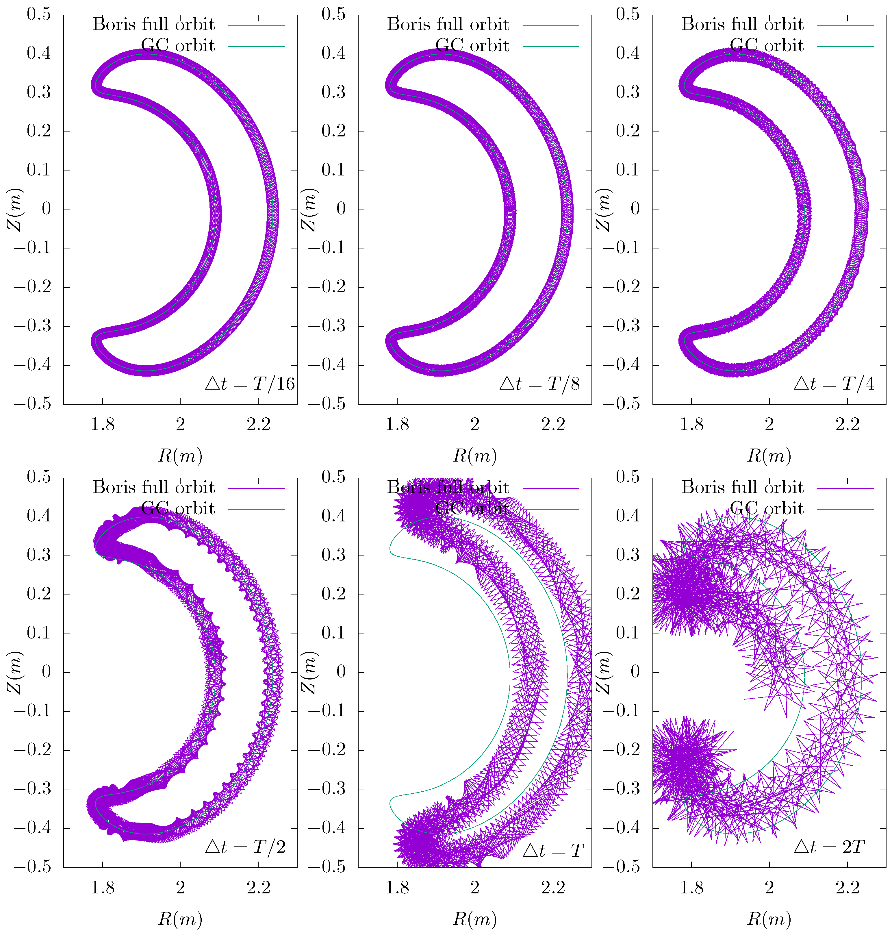
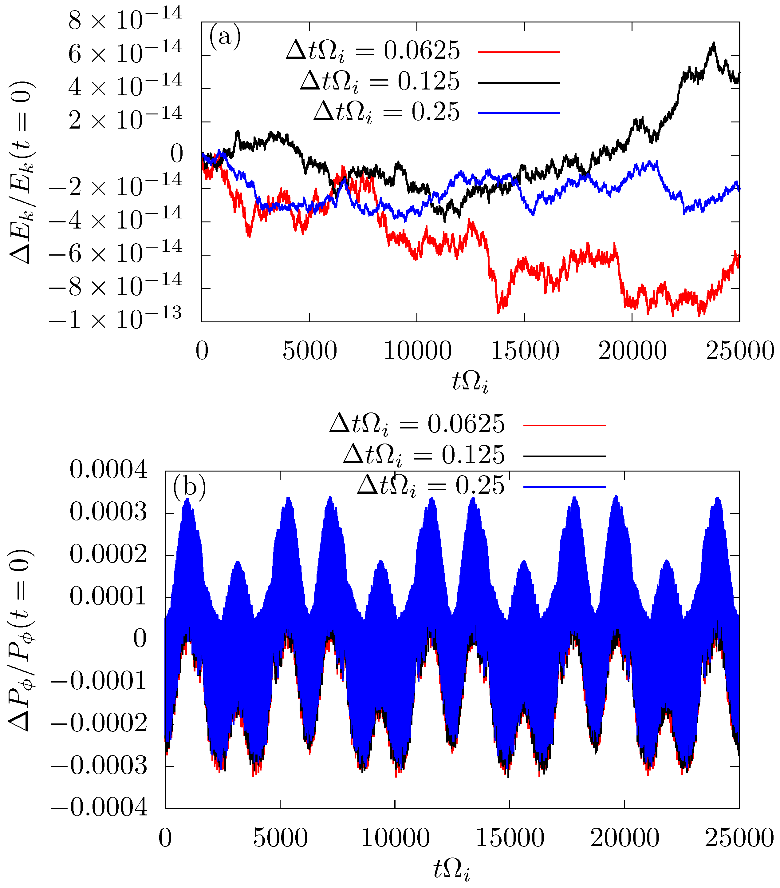
In this work, we focus on the electrostatic limit, in which $\delta \mathbf{B}$ is zero and $\delta \mathbf{E}=-\nabla \delta \mathsf{\Phi }$, where $\delta \mathsf{\Phi }$ is the perturbed electric potential. Furthermore, we adopt the simple adiabatic electron model for describing the electron response, in which the perturbed electron density is related to $\delta \mathsf{\Phi }$ by

$$\delta n_e=n_{e0}\frac{e(\delta \mathsf{\Phi }-\langle \delta \mathsf{\Phi }\rangle )}{T_{e0}},$$

(6)

where $n_{e0}$ and $T_{e0}$ are the equilibrium electron number density and temperature, respectively; e is the elementary charge, $\langle \dots \rangle$ is the magnetic surface averaging operator defined by

$$\langle \dots \rangle =\frac{{\int }_0^{2\pi }{\int }_{-\pi }^{+\pi }(\dots )\mathcal{J}d\varphi d\theta }{{\int }_0^{2\pi }{\int }_{-\pi }^{+\pi }\mathcal{J}d\varphi d\theta },$$

(7)

where $\mathcal{J}$ is the Jacobian of magnetic coordinates $(\psi ,\theta ,\varphi )$, $\psi$ is a radial coordinate, $\theta$ and $\varphi$ are poloidal and toroidal angles, respectively.

In the electrostatic limit, Maxwell’s equations reduce to Poisson’s equation, which further reduces to the quasi-neutrality condition if the space-charge term is neglected. The quasi-neutrality condition is written as

$$\delta n_e=\delta n_i$$

(8)

where $\delta n_i$ is the perturbed part of the ion number density. Using $\delta n_e$ given by Equation (6) in the above equation, we obtain

$$n_{e0}\frac{e(\delta \mathsf{\Phi }-\langle \delta \mathsf{\Phi }\rangle )}{T_e}=\delta n_i,$$

(9)

which serves as our field equation, from which the electric potential $\delta \mathsf{\Phi }$ can be solved. We consider modes with $n\ne 0$, where n is the toroidal mode number. Then the flux average $\langle \delta \mathsf{\Phi }\rangle$ is always zero and the field Equation (9) reduces to an algebraic equation, which can be analytically solved to give

$$\delta \mathsf{\Phi }=\frac{T_e}{e}\frac{\delta n_i}{n_{e0}}.$$

(10)

3. Implicit $\delta f$ Particle-in-Cell Method and Full Orbit Integrator

The ion Vlasov Equation (5) is solved by using the $\delta f$ PIC method [23,24], in which an assembly of markers are loaded in the phase-space according to a distribution function $g(\mathbf{x},\mathbf{v})$. Then the phase space volume occupied by a marker located at $({\mathbf{x}}_j,{\mathbf{v}}_j)$ is given by $V_{psj}=1/g({\mathbf{x}}_j,{\mathbf{v}}_j)$. We define the weight of the $jth$ marker by

$$w_{ij}=\delta f_i({\mathbf{x}}_j,{\mathbf{v}}_j)V_{psj}=\frac{\delta f_i({\mathbf{x}}_j,{\mathbf{v}}_j)}{g({\mathbf{x}}_j,{\mathbf{v}}_j)},$$

(11)

which is the physical particle number carried by $\delta f_i$ in the phase space volume $V_{psj}$. The weight evolution equation is obtained by multiplying both sides of Equation (5) by $V_{psj}$ and noting that $d\left(V_{psj}\right)/dt=0$, yielding

$$\begin{array}{ccc}\frac{d{w}_{ij}}{dt}\hfill & =\hfill & \frac{f_{i0}}{g}\frac{q_i}{T_i}\delta \mathbf{E}·\mathbf{v}\hfill \\ & +\hfill & \frac{f_{i0}}{g}\left[{\kappa }_{n_i}+\left(\frac{m{v}^2}{2T_i}-\frac{3}{2}\right){\kappa }_{T_i}\right]\frac{(\delta \mathbf{E}\times \mathbf{b})·\nabla r}{B_0},\hfill \end{array}$$

(12)

where the magnetic perturbation terms have been dropped due to the electrostatic approximation. An implicit scheme is used to integrate the weight evolution equation. Denoting the right-hand side of the weight evolution Equation (12) by $h(\delta \mathbf{E},\mathbf{x},\mathbf{v})$, the implicit scheme we use takes the following form:

$$\frac{w_{ij}^{(n+1)}-w_{ij}^{\left(n\right)}}{\Delta t}=h(\delta {\mathbf{E}}^{(n+1/2)},{\mathbf{x}}_j^{(n+1/2)},{\mathbf{v}}_j^{(n+1/2)}),$$

(13)

with

$$\delta {\mathbf{E}}^{(n+1/2)}=\frac{\delta {\mathbf{E}}^{(n+1)}+\delta {\mathbf{E}}^{\left(n\right)}}{2},$$

(14)

We choose the initial guess of $\delta {\mathbf{E}}^{(n+1)}$ to be equal to $\delta {\mathbf{E}}^{\left(n\right)}$ and then iterate until convergence is achieved. If the iteration is terminated after only two iterations, then this scheme corresponds to the predictor-corrector scheme called Heun’s method [25]. The field Equation (9) needs to be solved once in each iteration.

The ion trajectory $({\mathbf{x}}_j,{\mathbf{v}}_j)$ is advanced by a time-centered difference scheme given by

$$\frac{{\mathbf{v}}^{(n+1/2)}-{\mathbf{v}}^{(n-1/2)}}{\Delta t}=\frac{q_i}{m_i}\left[{\mathbf{E}}^{\left(n\right)}({\mathbf{x}}^{\left(n\right)})+\frac{{\mathbf{v}}^{(n+1/2)}+{\mathbf{v}}^{(n-1/2)}}{2}\times {\mathbf{B}}^{\left(n\right)}({\mathbf{x}}^{\left(n\right)})\right].$$

(15)

for velocity and

$$\frac{{\mathbf{x}}^{(n+1)}-{\mathbf{x}}^{\left(n\right)}}{\Delta t}={\mathbf{v}}^{(n+1/2)},$$

(16)

for position. Here “staggered” time grids are used for $\mathbf{v}$ and $\mathbf{x}$: time grids of $\mathbf{v}$ are at half-steps while time grids of $\mathbf{x}$ are at integer steps. The position at half-steps, ${\mathbf{x}}^{(n+1/2)}$, which is needed in Equation (13), is approximated by ${\mathbf{x}}^{(n+1/2)}=({\mathbf{x}}^{\left(n\right)}+{\mathbf{x}}^{(n+1)})/2$. Further note that the scheme given in Equation (15) is in an implicit form since the unknown ${\mathbf{v}}^{(n+1/2)}$ appears on both sides of the equation. Fortunately, Equation (15) can be analytically solved in Cartesian basis and its explicit solution is expressed by the Boris algorithm [26]. As is discussed in Ref. [27], the above scheme conserves the phase-space volume, which makes it suitable for particle-based methods where phase-space volume conservation is usually implicitly assumed. In this work, cylindrical coordinates are used in integrating the ion orbits. When implementing the Boris scheme in cylindrical coordinates, a local Cartesian coordinate system with basis vectors $({\mathbf{e}}_x,{\mathbf{e}}_y,{\mathbf{e}}_z)$ along the local cylindrical basis vectors $({\mathbf{e}}_R,{\mathbf{e}}_{\varphi },{\mathbf{e}}_Z)$ at particle location ${\mathbf{x}}^{\left(n\right)}$ is set up to perform the velocity integration to obtain ${\mathbf{v}}^{(n+1/2)}$. Then the particle location is updated in the local Cartesian coordinates by using Equation (16) and then is transformed to the cylindrical coordinates by using the analytic coordinate transformation. After this, the new velocity ${\mathbf{v}}^{(n+1/2)}$ is projected onto the new basis vectors $({\mathbf{e}}_R,{\mathbf{e}}_{\varphi },{\mathbf{e}}_Z)$ at particle location ${\mathbf{x}}^{(n+1)}$. Typical full ion orbits computed by this scheme are compared with the guiding center orbit in Figure 1. This scheme can reproduce correct drift motion even when a large time-step comparable to the gyro-period is used [28]. Figure 1 shows examples of orbits computed with large time steps.

Figure 2 plots the relative variation of the kinetic energy $E_k$ and toroidal angular momentum $P_{\varphi }$ computed by the Boris full orbit integrator over a time period of $t{\mathsf{\Omega }}_i=2.5\times {10}^4$ for different time step sizes in a tokamak equilibrium magnetic field, where ${\mathsf{\Omega }}_i$ is the ion cyclotron angular frequency at the magnetic axis. The results indicate that the kinetic energy conservation is accurate to the machine error and the relative error in the toroidal angular momentum conservation is within $0.04\%$. The kinetic energy conservation of the Boris integrator is much better than the variational integrator of Ref. [21]. This is because the Boris integrator directly rotates the velocity, which does not change the amplitude of the velocity when no electric field is present.

In the linear limit, the fields $\mathbf{E}$ and $\mathbf{B}$ on the right-hand side of Equation (15) are replaced by the equilibrium fields ${\mathbf{E}}_0$ and ${\mathbf{B}}_0$. In the present work, ${\mathbf{E}}_0=0$ and ${\mathbf{B}}_0$ is a general toroidal magnetic configuration specified numerically.

4. Magnetic Field Specification and Field-Line-Following Coordinates

The equilibrium magnetic field is specified numerically by reading and interpolating the output of the equilibrium reconstruction code EFIT [30]. This enables us to handle magnetic configurations with arbitrary flux surface shape.

A field-line-following coordinate system [31,32] $(\psi ,\theta ,\alpha )$ is constructed from the numerical magnetic configuration, with the radial coordinate $\psi$ being the normalized poloidal magnetic flux, $\theta$ being an equal-volume poloidal angle and $\alpha$ being a generalized toroidal angle defined by $\alpha =\varphi -{\int }_0^{\theta }\widehat{q}d\theta$, where $\varphi$ is the cylindrical toroidal angle, and $\widehat{q}=\mathbf{B}·\nabla \varphi /\mathbf{B}·\nabla \theta$ is the local safety factor. In $(\psi ,\theta ,\alpha )$ coordinate system, both $\nabla \psi$ and $\nabla \alpha$ are perpendicular the field lines, i.e., ${\mathbf{B}}_0·\nabla \psi =0$, and ${\mathbf{B}}_0·\nabla \alpha =0$. Furthermore, the gradient along the field line is written as

$${\mathbf{B}}_0·\nabla =-{\mathsf{\Psi }}^{\prime }{\mathcal{J}}^{-1}\frac{\partial }{\partial \theta },$$

(17)

where ${\mathsf{\Psi }}^{\prime }=d\mathsf{\Psi }/d\psi$ with $\mathsf{\Psi }=A_{\varphi }R$ the poloidal magnetic flux function, and $\mathcal{J}={(\nabla \psi \times \nabla \theta ·\nabla \alpha )}^{-1}$ is the Jacobian of the $(\psi ,\theta ,\alpha )$ coordinates.

Ion markers are loaded in the field-line-following coordinates $(\psi ,\theta ,\alpha )$. Ion trajectories are integrated in cylindrical coordinates $(R,\varphi ,Z)$ and then linearly interpolated to $(\psi ,\theta ,\alpha )$ coordinates to do the deposition in order to obtain the perturbed ion density at the spatial grids of $(\psi ,\theta ,\alpha )$ coordinates. At a grid point ${\mathbf{x}}_k$, the perturbed ion density is approximated by

$$\delta n_i\left({\mathbf{x}}_k\right)=\frac{1}{\Delta V_s}\sum _{j=1}^{N_p}{w}_{ij}S({\mathbf{x}}_k-{\mathbf{x}}_j),$$

(18)

where $N_p$ is the total number of markers loaded, $\Delta V_s=\mathcal{J}\left({\mathbf{x}}_k\right)\Delta \psi \Delta \theta \Delta \alpha$ is the volume of the spatial cell, $\Delta \psi$, $\Delta \theta$, and $\Delta \alpha$ are the grid point spacings in the $\psi$, $\theta$ and $\alpha$ direction respectively, S is the interpolating function defined as

$$S\left(\mathbf{x}\right)=S_{1D}\left(\frac{\psi }{\Delta \psi }\right)S_{1D}\left(\frac{\theta }{\Delta \theta }\right)S_{1D}\left(\frac{\alpha }{\Delta \alpha }\right),$$

(19)

with $S_{1D}$ being the first-order b-spline function given by

$$S_{1D}\left(x\right)=\left\{\begin{array}{cc}1-\left|x\right|& :\left|x\right|\le 1\\ 0& :\left|x\right|>1\end{array}\right.,$$

(20)

(then the deposition corresponds to a linear interpolation). In this work, the marker distribution function g is chosen as $g=f_{i0}{N}_p/\left(V_s{n}_{i0}\right)$, where $V_s$ the spatial volume of the computational box.

After solving the field equation for $\delta \mathsf{\Phi }$, the spatial differential of $\delta \mathsf{\Phi }$ is performed in the field-line-following coordinates to determine the perturbed electric field. The deposition and field solving are done in field-line-following coordinates because this coordinate system is efficient for resolving ITG modes, which have $k_{\parallel }\ll k_{\perp }$, where $k_{\parallel }$ and $k_{\perp }$ are the parallel and perpendicular wave-number, respectively.

5. Simulation Results of ITG Instabilities

To benchmark the results against those of Ref. [21], we adopt the DIII-D cyclone base case [29], which is a concentric-circular magnetic configuration. The main parameters used in the benchmarking are summarized in

Table 1. DIII-D cyclone base case parameters [29]. The safety factor profile is given by $q\left(r\right)=q_0+(r-r_0)q^{\prime }\left(r_0\right)$ with $q^{\prime }\left(r_0\right)=\widehat{s}{q}_0/r_0$, where $\widehat{s}$ is the magnetic shear at $r=r_0$ (the radial center of the simulation box). In this case, $R_0/{\rho }_i=450.5$, where ${\rho }_i=v_{ti}/{\mathsf{\Omega }}_i$ is the thermal ion gyro-radius at the magnetic axis, $v_{ti}=\sqrt{T_{i0}/m_i}$, ${\mathsf{\Omega }}_i=B_{axis}{q}_i/m_i$ is the ion cyclotron angular frequency at the magnetic axis. Deuterium plasma is assumed in our simulation.

${\mathit{R}}_0$	a	${\mathit{B}}_{axis}$	${\mathit{q}}_0$	$\widehat{\mathit{s}}$	${\mathit{r}}_0$	${\mathit{\kappa }}_{{\mathit{T}}_{\mathit{i}}}{\mathit{R}}_0$	${\mathit{\kappa }}_{{\mathit{n}}_{\mathit{i}}}{\mathit{R}}_0$	${\mathit{T}}_{\mathit{i}0}$	${\mathit{q}}_{\mathit{i}}{\mathit{T}}_{\mathit{i}0}/\left({\mathit{eT}}_{\mathit{e}0}\right)$
1.32 m	0.48 m	$1.91T$	1.40	0.78	0.24 m	6.9	2.2	1.5 keV	1

.

Although the DIII-D cyclone equilibrium is analytic and circular, the equilibrium is read in as a general equilibrium specified numerically in the G-EQDSK format of EFIT code. No analytic relations particular to this specific configuration is relied on.

The radial center of the simulation box is at $r=r_0=0.24$ m and the radial width $\Delta r=0.11$ m, which is about $37.5{\rho }_i$. The perturbed potential $\delta \mathsf{\Phi }$ is set to zero at the radial boundaries. When a marker moves out of the radial boundary, its vertical location is changed from Z to $-Z$ (this is to follow the drift orbit) and its weight is set to zero, where Z is the vertical coordinate of cylindrical coordinates.

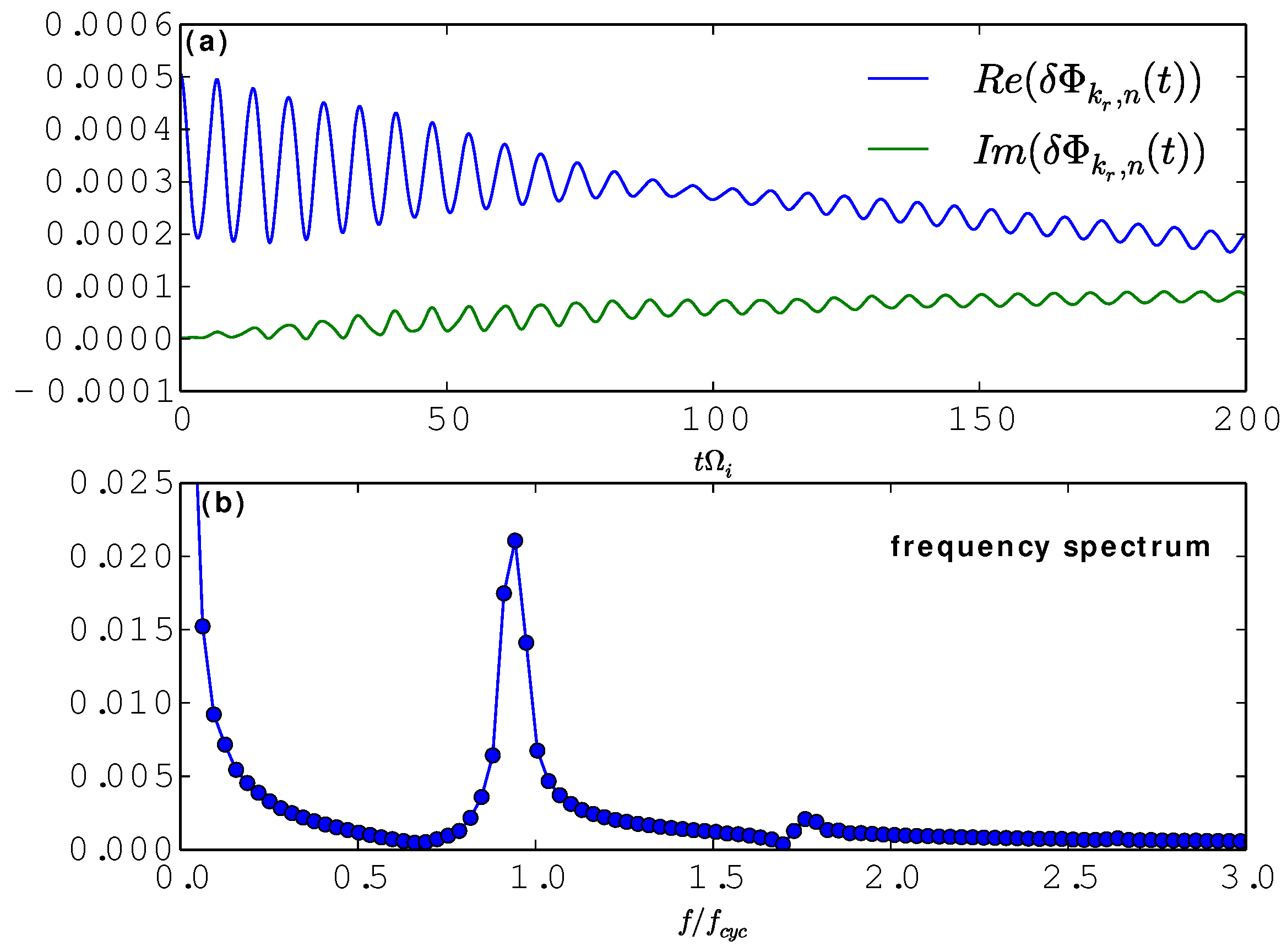
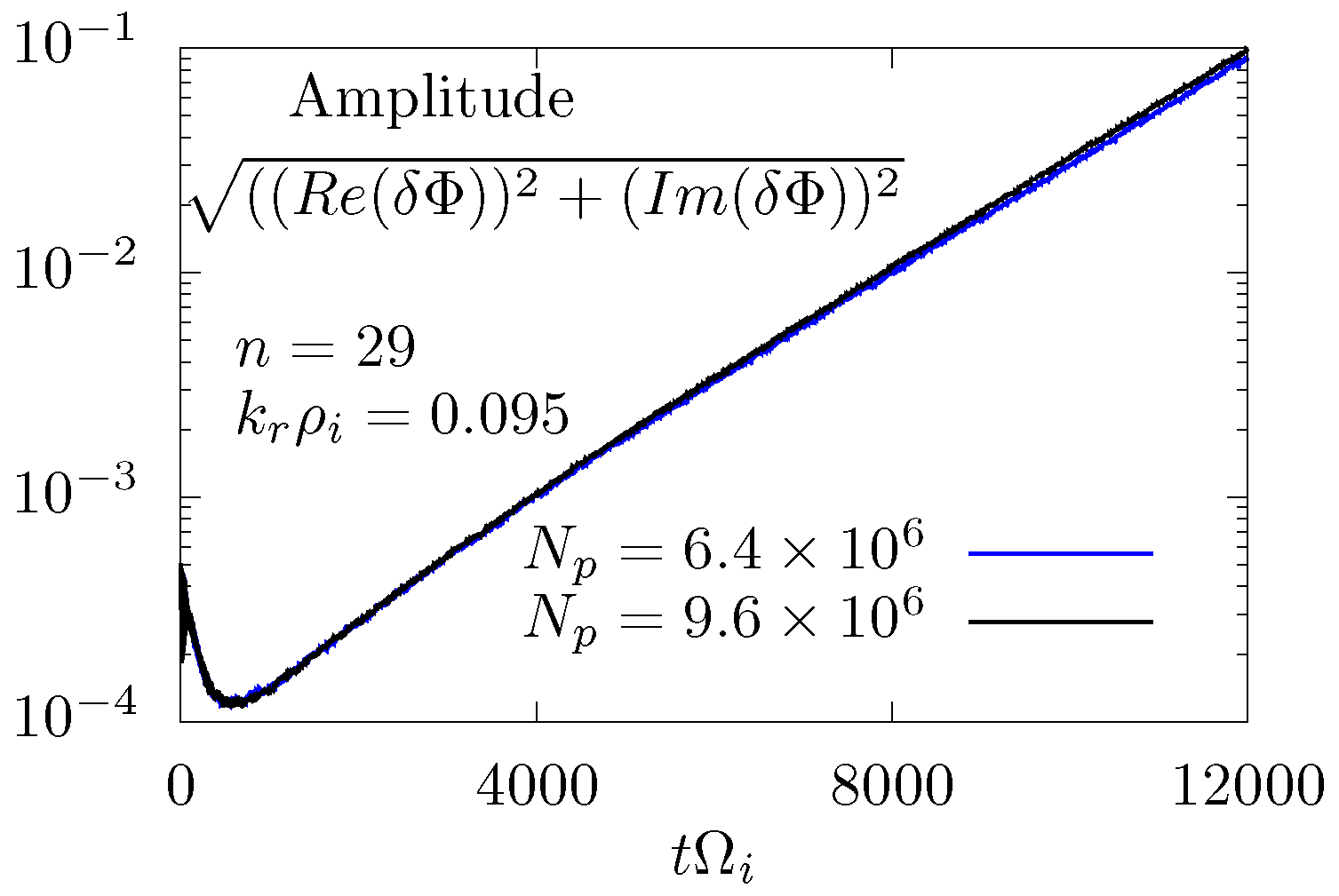
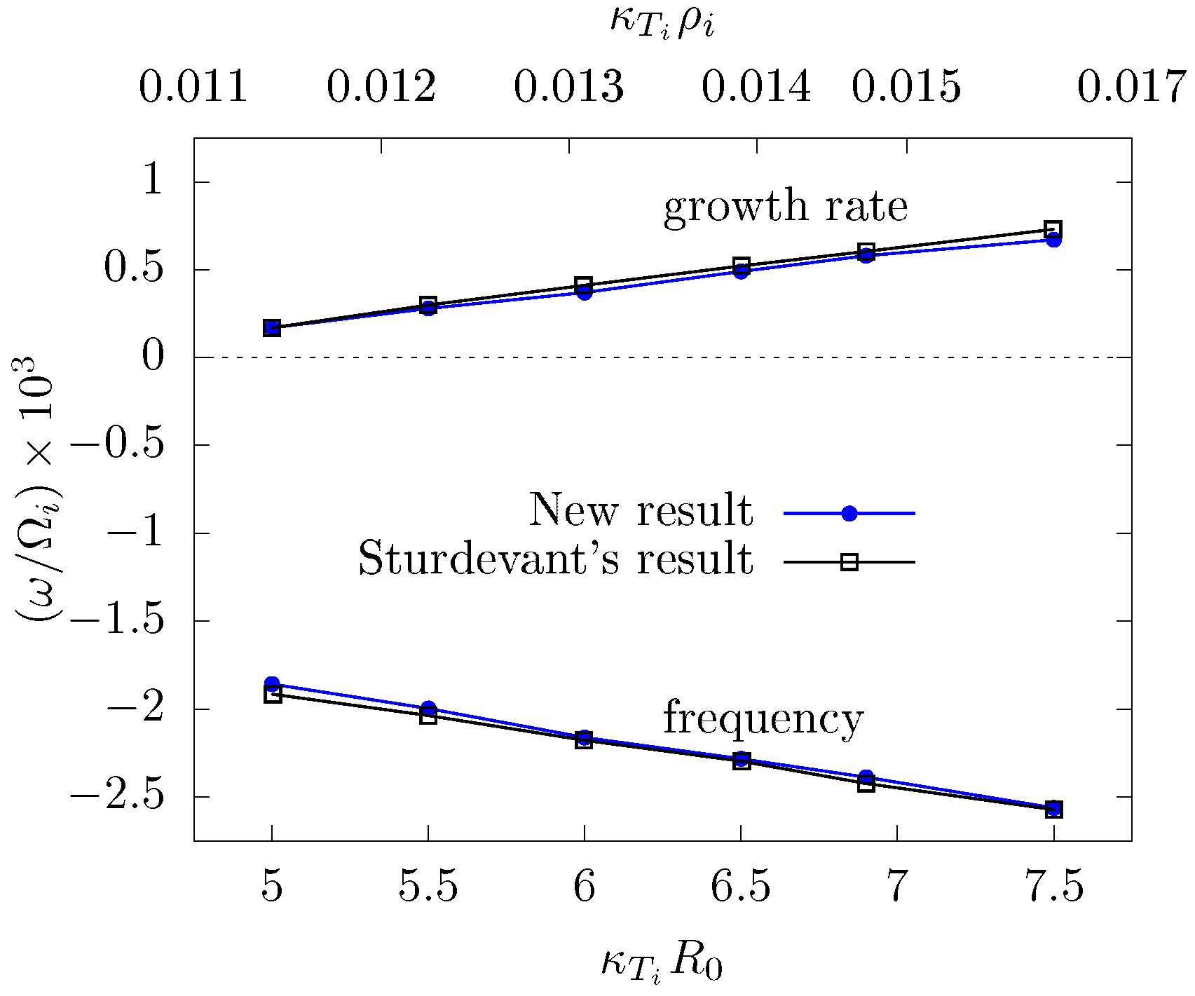
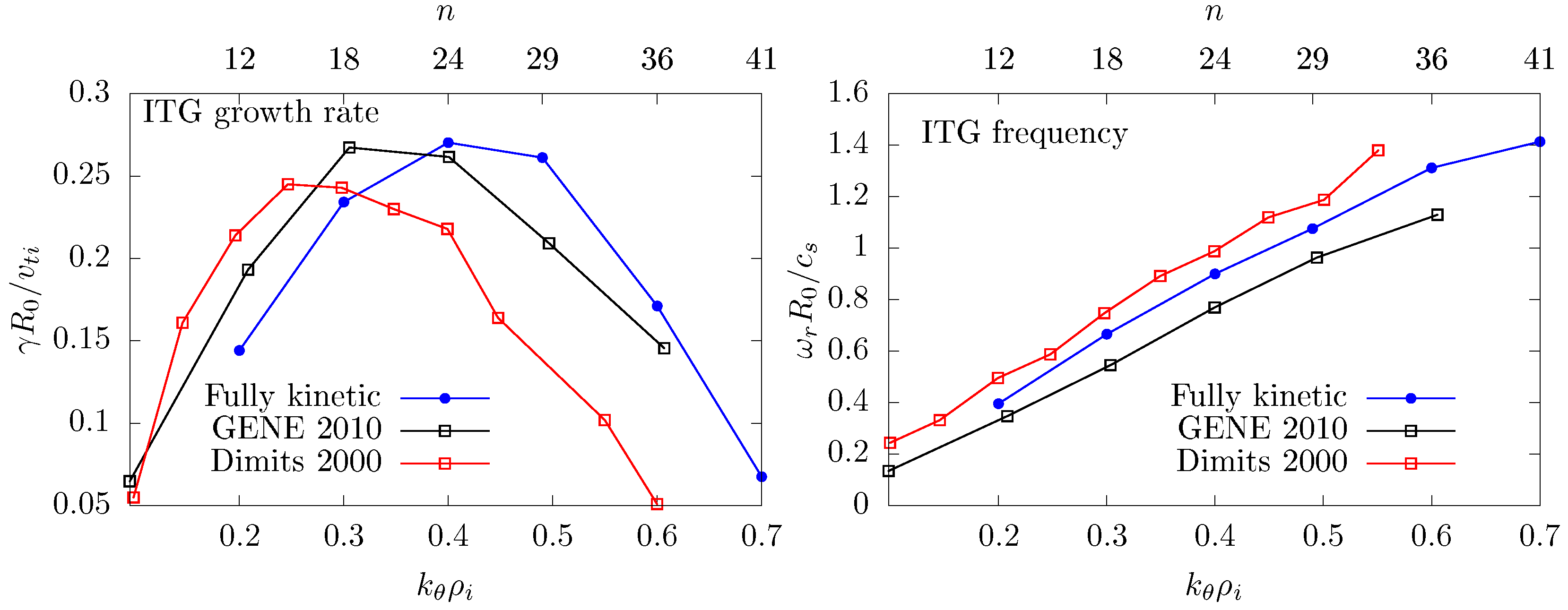
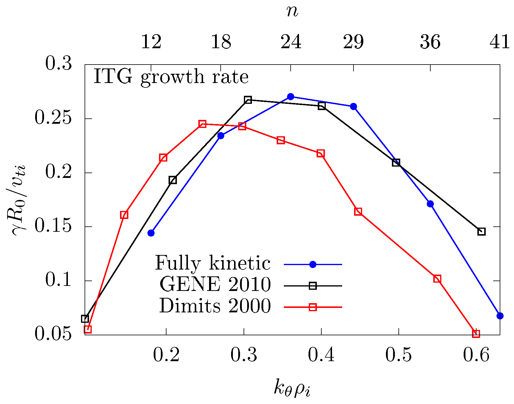
5.1. Linear Results of ITG Instabilities and Benchmarking with Other Codes

Figure 3 shows the time evolution of an $n=29$ linear ITG instability for DIII-D cyclone base case parameters. Clear exponential growth of the instability is observed. The frequency and growth rate in this case are ${\omega }_r/{\mathsf{\Omega }}_i=2.388\times {10}^{-3}$ and $\gamma /{\mathsf{\Omega }}_i=5.8\times {10}^{-4}$ while the corresponding results from Ref. [21] are ${\omega }_r/{\mathsf{\Omega }}_i=2.423\times {10}^{-3}$ and $\gamma /{\mathsf{\Omega }}_i=6.0\times {10}^{-4}$.

This is a multi-scale simulation, which includes both the slow-scale ITG instability and the fast-scale wave associated with the ion gyro-motion. In the simulation, we can identify the existence of the ion Bernstein wave (IBW) associated with the ion gyro-motion. The IBW is hidden in the simulation in Figure 3, the details of which are plotted in Figure 4a for $t{\mathsf{\Omega }}_i=[0:200]$. The corresponding frequency spectrum is plotted in Figure 4b, which shows a clear peak near the ion gyro-frequency.

Numerical parameters used in obtaining the above and the following results are as follows: the time step $\Delta t{\mathsf{\Omega }}_i=0.2$, the spatial resolution in $(\psi ,\theta ,\alpha )$ is $(162,64,32)$, where the toroidal range is a wedge with $\Delta \alpha =2\pi /n$, the number of total markers $N_p=6.4\times {10}^6$ (the number of markers per cell is about 19). Increasing the number of markers to $N_p=9.6\times {10}^6$ produced no significant difference in the growth rate, as is shown in Figure 5.

The code uses one dimensional domain decomposition along $\theta$ and 4 MPI processes are used for particle parallelization for each $\theta$ cell and thus total $64\times 4=256$ MPI processes are used. The code run on NERSC Cori system and typical runs use eight Intel Xeon “Haswell” nodes, each of which is equipped with 32 physical cores supporting 2 hyper-threads and thus $2\times 32=64$ logical cores. The code uses OpenMP to make use of this hyper-threading capability. For the above run with $6\times {10}^4$ time-steps, the wall-time is $2.3$ h. (Each Cori node has two sockets and each socket is populated with a 16-core Intel${}^{\circledR }$ Xeon™ Processor E5-2698 v3 at 2.3 GHz.)

Figure 6 presents the dependence of the linear ITG mode frequency and growth rate on the ion temperature gradient ${\kappa }_{T_i}$, which shows that both the frequency and growth rate increase with the temperature gradient drive. Also plotted in Figure 6 are the fully kinetic results from Ref. [21], which are in good agreement with our new results.

Gyrokinetic simulations found that ITG instabilities usually reach a peak growth rate near a particular toroidal mode number n in the scanning over n, which is often represented in terms of the bi-normal wave-number $k_{\theta }$ defined by $k_{\theta }\approx n{q}_0/r_0$. This trend can also be captured by the fully kinetic ion model. Figure 7 shows the dependence of ITG growth rate and frequency on $k_{\theta }{\rho }_i$ given by the fully kinetic model, which shows that the growth rate reaches a peak near $k_{\theta }{\rho }_i\approx 0.4$. Also plotted in Figure 7 are the gyrokinetic results from Ref. [22,29], which roughly agree with our results. The difference between our results and those from GENE 2010 (Ref. [22]) is mainly due to the difference in the value of the thermal ion gyro-radius at the magnetic axis ${\rho }_i$. In our simulation, ${\rho }_i=R_0/450.5$, while ${\rho }_i=R_0/500.0$ in Ref. [22]. Without redoing the simulation, we re-plot the results by using $k_{\theta }{\rho }_i$ consistent with that of GENE 2010, yielding the results in Figure 8, which shows better agreement between our results and GENE 2010. Several other factors may also contribute to the difference between the three results. Safety factor profiles are slightly different: $q\left(r\right)=q_0+(r-r_0)q^{\prime }\left(r_0\right)$ in this work, while $q\left(r\right)=0.86-0.16r/a+2.52{(r/a)}^2$ in Ref. [22] and q profile variation is neglected in the flux-tube model of Ref. [29]. The radial variation of the density and temperature is neglected in the present work and Ref. [29] while Ref. [22] includes the density and temperature profile. Deuterium plasma is used in our simulation.

Figure 9 plots the two-dimensional mode structure of the $n=29$ ITG instability in the poloidal plane, which shows a clear ballooning structure (i.e., the amplitude on the low-field-side is larger than that on the high-field-side). This is consistent with the physical picture that ITG instabilities are driven by the $E\times B$ drift on the tokamak low-field-side while the $E\times B$ drift on the high-field side (the “good-curvature” side ) suppresses the instabilities.

5.2. Nonlinear Results of ITG Instabilities and Analysis of Saturation due to $E\times B$ Trapping

With the Boris integrator, it is straightforward to extend the adiabatic electron model to the nonlinear regime, by including the electric field terms in the integration of particle trajectories. In a single-n simulation, the ITG instability saturates due to the $\mathbf{E}\times \mathbf{B}$ trapping, as discussed in Ref. [20] for slab geometry. Figure 10 plots the nonlinear evolution of the $n=29$ ITG instability, along with the $\mathbf{E}\times \mathbf{B}$ trapping prediction for the saturation amplitude.

The instability is expected to saturate when the $\mathbf{E}\times \mathbf{B}$ trapping angular frequency ${\omega }_{E\times B}$ becomes as large as the instability growth rate, i.e.,

$${\omega }_{E\times B}\approx \gamma ,$$

(21)

where ${\omega }_{E\times B}$ is proportional to the amplitude of $\delta \mathsf{\Phi }$. The trapping frequency ${\omega }_{E\times B}$ can be estimated by calculating the time for a particle with the $\mathbf{E}\times \mathbf{B}$ drift velocity to go around the eddies of the potential $\delta \mathsf{\Phi }$. The circumference l of the $\delta \mathsf{\Phi }$ eddies in the poloidal plane can be estimated as the fundamental radial wave-length in the sine expansion, i.e., $l\approx \pi /k_r$. The $\delta \mathbf{E}\times {\mathbf{B}}_0$ drift is given by

$${\mathbf{V}}_{E\times B}=\frac{\delta \mathbf{E}\times \mathbf{b}}{{\mathbf{B}}_0}=-\frac{\nabla \delta \mathsf{\Phi }\times \mathbf{b}}{{\mathbf{B}}_0},$$

(22)

which is along the contours of $\delta \mathsf{\Phi }$. Using the bi-normal wavenumber $k_{\theta }=n{q}_0/r_0$ to estimate the gradient of $\delta \mathsf{\Phi }$, then the magnitude of the $\delta \mathbf{E}\times {\mathbf{B}}_0$ drift can be estimated as

$$V_{E\times B}\approx \frac{\delta \mathsf{\Phi }}{B_0}\frac{n{q}_0}{r_0}.$$

(23)

Then the $\delta \mathbf{E}\times {\mathbf{B}}_0$ trapping angular frequency can be written as

$${\omega }_{E\times B}=\frac{2\pi }{T_{E\times B}}=\frac{2\pi V_{E\times B}}{l}\approx 2\frac{\delta \mathsf{\Phi }}{B_0}\frac{n{q}_0}{r_0}{k}_r.$$

(24)

Using this expression, the saturation amplitude $\delta {\mathsf{\Phi }}_s$ predicted by the critical condition (21) is written as

$$\delta {\mathsf{\Phi }}_s\approx \gamma B_0\frac{1}{2k_r}\frac{r_0}{n{q}_0}.$$

(25)

Then the normalized potential $e\delta {\mathsf{\Phi }}_s/T_e$ is written as

$$\frac{e}{T_e}\delta {\mathsf{\Phi }}_s\approx \frac{\gamma }{{\mathsf{\Omega }}_i}\frac{1}{2k_r{\rho }_i}\frac{r_0/{\rho }_i}{n{q}_0}.$$

(26)

Using $\gamma /{\mathsf{\Omega }}_i=5.8\times {10}^{-4}$, $k_r{\rho }_i=0.095$, $r_0/{\rho }_i=81.9$, $n=29$, and $q_0=1.4$, the above formula gives $e\delta {\mathsf{\Phi }}_s/T_e=6.16\times {10}^{-3}$. As is shown in Figure 10, this estimation roughly agrees with the saturation amplitude observed in the simulation.

Physically, the dominant saturation mechanism of ITG instability is the nonlinear generation of an $n=0$ zonal flow, which suppresses the ITG instability through radial shear. With fully kinetic ions, the adiabatic electron model gives no explicit equation for the $\delta \mathsf{\Phi }$ with $n=0$, making it difficult to solve the field equation, so we do not demonstrate that mechanism here. Extended models to capture this effect are the subject of ongoing investigation. Ref. [20] included the electron polarization response to model the $n=0$ response. Another option is to use the ion momentum equation to indirectly enforce quasi-neutrality. These models are outside the scope of this work.

6. Summary

The viability of the fully kinetic ion model in simulating the low-frequency ITG instability in tokamaks is demonstrated in this work by using the toroidal Boris full orbit integrator. The equilibrium full orbits computed by this integrator conserve the kinetic energy accurate to the round-off error and the relative error in the toroidal angular momentum conservation is within $0.04\%$ over a time period of $t{\mathsf{\Omega }}_i=2.5\times {10}^4$. This work extends the previous work to the nonlinear regime and investigates the nonlinear saturation of a single-n ITG instability due to the $E\times B$ trapping mechanism. The saturation amplitude predicted by the $E\times B$ trapping is found to agree with the saturation level observed in the simulation. This work also extends the previous work from analytic circular magnetic equilibria to general magnetic equilibria, enabling simulation of realistic equilibria reconstructed from tokamak experiments.

This work is limited to the electrostatic case with the simple adiabatic electron model. The nonlinear case reported in this paper is limited to the saturation of a single-n mode. Future work will consider electromagnetic effects using more accurate drift-kinetic model for electrons. The nonlinear case will be extended to include interactions between ITG modes of multiple toroidal mode numbers and their coupling to the zonal flow.

The Fortran code used in obtaining the results presented in this work is released as an open-source software under the GNU General Public License v3.0. The source code can be downloaded from: https://github.com/Youjunhu/Fully_kinetics_tokamak_ITG.

References

1. Guzdar, P.N.; Chen, L.; Tang, W.M.; Rutherford, P.H. Ion-temperature-gradient instability in toroidal plasmas. Phys. Fluids 1983, 26, 673–677. [Google Scholar] [CrossRef]
2. Rettig, C.L.; Rhodes, T.L.; Leboeuf, J.N.; Peebles, W.A.; Doyle, E.J.; Staebler, G.M.; Burrell, K.H.; Moyer, R.A. Search for the ion temperature gradient mode in a tokamak plasma and comparison with theoretical predictions. Phys. Plasmas 2001, 8, 2232–2237. [Google Scholar] [CrossRef]
3. Lin, Z.; Hahm, T.S.; Lee, W.W.; Tang, W.M.; White, R.B. Turbulent Transport Reduction by Zonal Flows: Massively Parallel Simulations. Science 1998, 281, 1835–1837. [Google Scholar] [CrossRef] [PubMed]
4. Xie, H.S.; Xiao, Y.; Lin, Z. New Paradigm for Turbulent Transport Across a Steep Gradient in Toroidal Plasmas. Phys. Rev. Lett. 2017, 118, 095001. [Google Scholar] [CrossRef] [PubMed]
5. Parker, S.E.; Lee, W.W.; Santoro, R.A. Gyrokinetic simulation of ion temperature gradient driven turbulence in 3D toroidal geometry. Phys. Rev. Lett. 1993, 71, 2042–2045. [Google Scholar] [CrossRef] [PubMed]
6. Idomura, Y.; Tokuda, S.; Kishimoto, Y. Global gyrokinetic simulation of ion temperature gradient driven turbulence in plasmas using a canonical Maxwellian distribution. Nucl. Fusion 2003, 43, 234. [Google Scholar] [CrossRef]
7. Gao, Z.; Sanuki, H.; Itoh, K.; Dong, J.Q. Short wavelength ion temperature gradient instability in toroidal plasmas. Phys. Plasmas 2005, 12, 022502. [Google Scholar] [CrossRef]
8. Chen, Y.; Parker, S.E. Electromagnetic gyrokinetic δf particle-in-cell turbulence simulation with realistic equilibrium profiles and geometry. J. Comput. Phys. 2007, 220, 839–855. [Google Scholar] [CrossRef]
9. Ye, L.; Xu, Y.; Xiao, X.; Dai, Z.; Wang, S. A gyrokinetic continuum code based on the numerical Lie transform (NLT) method. J.Comput. Phys. 2016, 316, 180–192. [Google Scholar] [CrossRef]
10. Görler, T.; Lapillonne, X.; Brunner, S.; Dannert, T.; Jenko, F.; Merz, F.; Told, D. The global version of the gyrokinetic turbulence code GENE. J. Comput. Phys. 2011, 230, 7053–7071. [Google Scholar] [CrossRef]
11. Ku, S.; Chang, C.; Diamond, P. Full-f gyrokinetic particle simulation of centrally heated global ITG turbulence from magnetic axis to edge pedestal top in a realistic tokamak geometry. Nucl. Fusion 2009, 49, 115021. [Google Scholar] [CrossRef]
12. Chang, C.S.; Ku, S.; Tynan, G.R.; Hager, R.; Churchill, R.M.; Cziegler, I.; Greenwald, M.; Hubbard, A.E.; Hughes, J.W. Fast Low-to-High Confinement Mode Bifurcation Dynamics in a Tokamak Edge Plasma Gyrokinetic Simulation. Phys. Rev. Lett. 2017, 118, 175001. [Google Scholar] [CrossRef] [PubMed]
13. Chen, Y.; Parker, S.E. Particle-in-cell simulation with Vlasov ions and drift kinetic electrons. Phys. Plasmas 2009, 16, 052305. [Google Scholar] [CrossRef]
14. Belova, E.V.; Gorelenkov, N.N.; Cheng, C.Z. Self-consistent equilibrium model of low aspect-ratio toroidal plasma with energetic beam ions. Physics of Plasmas 2003, 10, 3240–3251. [Google Scholar] [CrossRef]
15. Lin, Y.; Wang, X.Y.; Chen, L.; Lu, X.; Kong, W. An improved gyrokinetic electron and fully kinetic ion particle simulation scheme: Benchmark with a linear tearing mode. Plasma Phys. Controll. Fusion 2011, 53, 054013. [Google Scholar] [CrossRef]
16. Waltz, R.E.; Deng, Z. Nonlinear theory of drift-cyclotron kinetics and the possible breakdown of gyro-kinetics. Phys. Plasmas 2013, 20, 012507. [Google Scholar] [CrossRef]
17. Kramer, G.J.; Budny, R.V.; Bortolon, A.; Fredrickson, E.D.; Fu, G.Y.; Heidbrink, W.W.; Nazikian, R.; Valeo, E.; Zeeland, M.A.V. A description of the full-particle-orbit-following SPIRAL code for simulating fast-ion experiments in tokamaks. Plasma Phys. Controll. Fusion 2013, 55, 025013. [Google Scholar] [CrossRef]
18. Kuley, A.; Lin, Z.; Bao, J.; Wei, X.S.; Xiao, Y.; Zhang, W.; Sun, G.Y.; Fisch, N.J. Verification of nonlinear particle simulation of radio frequency waves in tokamak. Phys. Plasmas 2015, 22, 102515. [Google Scholar] [CrossRef]
19. Sturdevant, B.J.; Parker, S.E.; Chen, Y.; Hause, B.B. An implicit δf particle-in-cell method with sub-cycling and orbit averaging for Lorentz ions. J. Comput. Phys. 2016, 316, 519–533. [Google Scholar] [CrossRef]
20. Miecnikowski, M.T.; Sturdevant, B.J.; Chen, Y.; Parker, S.E. Nonlinear saturation of the slab ITG instability and zonal flow generation with fully kinetic ions. Phys. Plasmas 2018, 25, 055901. [Google Scholar] [CrossRef]
21. Sturdevant, B.J.; Chen, Y.; Parker, S.E. Low frequency fully kinetic simulation of the toroidal ion temperature gradient instability. Phys. Plasmas 2017, 24, 081207. [Google Scholar] [CrossRef]
22. Lapillonne, X.; McMillan, B.F.; Görler, T.; Brunner, S.; Dannert, T.; Jenko, F.; Merz, F.; Villard, L. Nonlinear quasisteady state benchmark of global gyrokinetic codes. Phys. Plasmas 2010, 17, 112321. [Google Scholar] [CrossRef]
23. Parker, S.E.; Lee, W.W. A fully nonlinear characteristic method for gyrokinetic simulation. Phys. Fluid. B Plasma Phys. 1993, 5, 77–86. [Google Scholar] [CrossRef]
24. Aydemir, A.Y. A unified Monte Carlo interpretation of particle simulations and applications to non-neutral plasmas. Phys. Plasmas 1994, 1, 822–831. [Google Scholar] [CrossRef]
25. Süli, E.; Mayers, D.F. An Introduction to Numerical Analysis; Cambridge University Press: Cambridge, UK, 2003. [Google Scholar]
26. Birdsall, C.; Langdon, A. Plasma Physics via Computer Simulation; CRC Press: Bocaton, FL, USA, 2004. [Google Scholar]
27. Qin, H.; Zhang, S.; Xiao, J.; Liu, J.; Sun, Y.; Tang, W.M. Why is Boris algorithm so good? Phys. Plasmas 2013, 20, 084503. [Google Scholar] [CrossRef]
28. Parker, S.; Birdsall, C. Numerical error in electron orbits with large ωceΔt. J. Comput. Phys. 1991, 97, 91–102. [Google Scholar] [CrossRef]
29. Dimits, A.M.; Bateman, G.; Beer, M.A.; Cohen, B.I.; Dorland, W.; Hammett, G.W.; Kim, C.; Kinsey, J.E.; Kotschenreuther, M.; Kritz, A.H.; et al. Comparisons and physics basis of tokamak transport models and turbulence simulations. Phys. Plasmas 2000, 7, 969–983. [Google Scholar] [CrossRef]
30. Lao, L.; John, H.S.; Stambaugh, R.; Kellman, A.; Pfeiffer, W. Reconstruction of current profile parameters and plasma shapes in tokamaks. Nucl. Fusion 1985, 25, 1611. [Google Scholar] [CrossRef]
31. Beer, M.A.; Cowley, S.C.; Hammett, G.W. Field-aligned coordinates for nonlinear simulations of tokamak turbulence. Phys. Plasmas 1995, 2, 2687–2700. [Google Scholar] [CrossRef]
32. Chen, Y.; Parker, S.E. A delta-f particle method for gyrokinetic simulations with kinetic electrons and electromagnetic perturbations. J. Comput. Phys. 2003, 189, 463–475. [Google Scholar] [CrossRef]
Figure 1. Comparison between the full orbits calculated by the Boris scheme with different time step sizes: Δ t = T / 16 , Δ t = T / 8 , Δ t = T / 4 , Δ t = T / 2 , Δ t = T , and Δ t = 2 T , where T is the ion (Deuteron) gyro-period at its initial location ( R = 2.1 m, Z = 0 m, ϕ = 0 ). The results show that the full orbits agrees with the guiding-center orbit for the cases with time-step Δ t < T / 4 . When Δ t is further increased, the computed full orbits deviate from the guiding-center orbit. Further note that the gyro-radius obtained remains nearly the same when the time-step Δ t < T / 4 . When Δ t is further increased, the gyro-radius becomes larger than the correct value. The magnetic configuration is from EAST tokamak discharge#[email protected]. The initial velocity is given by v R = v Z = 1.0 × 10 6 m/s, and v ϕ = 5 × 10 5 m/s, where ( v R , v ϕ , v Z ) are the velocity components in the cylindrical coordinate system. This corresponds to a kinetic energy of 23 keV . For Δ t = T / 16 , the orbit is advanced by 23,250 time-steps, in which the particle finishes one banana period.
Plasma 01 00010 g001
Figure 2. The relative variation of the kinetic energy (a) and toroidal angular momentum (b) given by the Boris full orbit integrator over a time period of t Ω i = 2.5 × 10 4 for different time step sizes in a tokamak equilibrium magnetic field. The initial conditions of the orbit are R = 1.176 R 0 , Z = 3.912 × 10 3 R 0 , v R = 3.371 × 10 3 R 0 Ω i , v Z = 3.371 × 10 3 R 0 Ω i , and v ϕ = 1.798 × 10 3 R 0 Ω i , where R 0 = 1.32 m and the magnetic configuration is the DIII-D cyclone base case, which is specified in Table 1. The toroidal angular momentum is defined by P ϕ = m i R v ϕ + q i Ψ , where Ψ is the poloidal magnetic flux function.
Plasma 01 00010 g002
Figure 3. Time evolution of an n = 29 linear ITG instability for DIII-D cyclone base case parameters. In the simulation, the perturbed electric potential δ Φ is Fourier filtered along the toroidal direction to retain only the n = 29 harmonic, which is further sine transformed along the radial direction and only low radial harmonics are retained. Shown here is the fundamental radial sine harmonic of δ Φ near the low-field-side midplane, which corresponds to k r ρ i = 0.095 . δ Φ is normalized by T e / e . The frequency and growth rate in this case are ω r / Ω i = 2.388 × 10 3 and γ / Ω i = 5.8 × 10 4 , which correspond to the fifth data point in Figure 6, where the corresponding results from Ref. [21] are ω r / Ω i = 2.423 × 10 3 and γ / Ω i = 6.0 × 10 4 .
Plasma 01 00010 g003
Figure 4. Time evolution (a) of the electric potential during t Ω i = [ 0 : 200 ] and the corresponding frequency spectrum (b), which shows a clear peak near the ion gyro-frequency. Here f cyc = Ω i / 2 π .
Plasma 01 00010 g004
Figure 5. Comparison of ITG instabilities computed with different marker numbers N p = 6.4 × 10 6 and N p = 9.6 × 10 6 . Other parameters are the same as those in Figure 3.
Plasma 01 00010 g005
Figure 6. Dependence of ITG mode frequency and growth rate on the ion temperature gradient κ T i for the DIII-D cyclone base case. The upper horizontal axis shows the ion temperature gradient normalized by the thermal ion gyro-radius. Also plotted are the results from Ref. [21], which are in good agreement with our new results.
Plasma 01 00010 g006
Figure 7. Dependence of ITG mode growth rate and frequency on k θ ρ i for DIII-D cyclone base case. The upper horizontal axis shows the corresponding toroidal mode number n. Also plotted are the gyrokinetic results reported in Ref. [22,29].
Plasma 01 00010 g007
Figure 8. A re-plot of the results in Figure 7. The only modification is that the value of k θ ρ i used in plotting the fully kinetic results is scaled by a factor of 450.5 / 500.0 to take into account the different values of ρ i used in the simulation. In this case, the only significant discrepancy between the fully kinetic results and GENE 2010 is at the last data point, which has a small growth rate and may be subject to a larger numerical error.
Plasma 01 00010 g008
Figure 9. Mode structure of the n = 29 ITG instability in the poloidal plane. Plotted here is the perturbed electric potential δ Φ at t Ω i = 12,000.
Plasma 01 00010 g009
Figure 10. Nonlinear saturation of the n = 29 ITG instability in the DIII-D cyclone base case. The perturbed potential δ Φ (normalized by T e / e ) is measured on the low-field-side midplane and averaged over the radial domain. The blue line shows the saturation predicted by the E × B trapping formula (26), which gives e δ Φ s / T e = 6.16 × 10 3 for this case.
Plasma 01 00010 g010