Development of a Gyrokinetic Particle-in-Cell Code for Whole-Volume Modeling of Stellarators

Abstract

We present initial results in the development of a gyrokinetic particle-in-cell code for the whole-volume modeling of stellarators. This is achieved through two modifications to the X-point Gyrokinetic Code (XGC), originally developed for tokamaks. One is an extension to three-dimensional geometries with an interface to Variational Moments Equilibrium Code (VMEC) data. The other is a connection between core and edge regions that have quite different field-line structures. The VMEC equilibrium is smoothly extended to the edge region by using a virtual casing method. Non-axisymmetric triangular meshes in which triangle nodes follow magnetic field lines in the toroidal direction are generated for field calculation using a finite-element method in the entire region of the extended VMEC equilibrium. These schemes are validated by basic benchmark tests relevant to each part of the calculation cycle, that is, particle push, particle-mesh interpolation, and field solver in a magnetic field equilibrium of Large Helical Device including the edge region. The developed code also demonstrates collisionless damping of geodesic acoustic modes and steady states with residual zonal flow in the core region.

1. Introduction

Gyrokinetic simulation is a powerful tool to explore kinetic plasma dynamics with a scale comparable to magnetic fusion devices, and it is widely used to investigate anomalous and neoclassical transport phenomena in the core region, where centrally heated plasmas and energetic particles are primarily confined. On the other hand, phenomenological fluid models are mainly employed for the edge region where the hot plasma makes contact with material walls along open magnetic field lines. The edge plasma dynamics play a crucial role in determining the performance of confinement devices through nonlocal interaction with core plasma dynamics, wall erosion and the resulting contamination of core plasmas [1]. Edge plasma dynamics such as suppression of edge turbulence and steepening of pressure gradient are observed during the transport bifurcation to a desired plasma state called high-confinement mode (H-mode) with improved particle and energy confinement times in Tokamaks [2,3].

Edge plasma simulation based on the gyrokinetic approach is needed to take high-fidelity edge physics that includes non-Maxwellian particle distribution, complicated orbit effects near X-point, and edge micro-turbulence into account in the detailed estimation of divertor heat load [4]. In addition, such simulation can be integrated with core transport simulations and is useful to consider the core–edge coupling relevant to the H-mode operation and heat balance between core heating and divertor heat exhaust. X-point Gyrokinetic Code (XGC) is a particle-in-cell gyrokinetic simulation code developed for whole-volume modeling of tokamaks [5,6]. Two features of edge plasma dynamics make it difficult to demonstrate them in the framework of gyrokinetic simulation. One is the non-Maxwellian distribution of edge plasma due to direct interaction with material walls. Total-f scheme is employed in XGC to address this difficulty. This scheme combines the fine-grained delta-f particle-in-cell scheme with a Eulerian description of background plasma dynamics in coarse-grained five-dimensional phase space [7,8,9]. This approach enables us to demonstrate non-Maxwellian dynamics without serious noise problems. The other is the complicated geometries of open magnetic field lines, including X-points and the mechanical components of the vacuum vessel. Perturbed field values and plasma fluid moments are evaluated on unstructured triangular mesh generated in accordance with the equilibrium magnetic field and realistic shape of vessel components [10]. Field equations are solved by a finite element field solver with the PETSc library [11].

The present work is to extend XGC to whole-volume gyrokinetic modeling of stellarators [12]. There are a few versions in the XGC code family [13], namely XGC0 [14], XGCa [15] and XGC1 [16]. The present development originates from a Fortran source code of XGC1 which includes XGCa features. XGCa is version of XGC1 that is streamlined for neoclassical physics with an axisymmetric field solver. A comprehensive computational and algorithmic description of the latest version XGC1 can be found in Refs. [17,18] Difficulties in this extension come from the complexity of the equilibrium magnetic field. The complexity includes the non-axisymmetry and stochastic structure of the edge magnetic field [19]. The core–edge coupling and H-mode transition in stellarators [20] are not fully understood under the effects of the stochastic structures. A gyrokinetic approach including anisotropic plasma dynamics and finite Larmor radius effect is needed to explore these issues.

In tokamaks, a smooth two-dimensional flux function can be obtained from EFIT equilibrium reconstruction [21] or other equilibrium models for the entire device domain. A triangular mesh generated from the flux function is applied to every poloidal cross section in this case. Solutions to the stellarator equilibrium problem are more complex due to the three-dimensional nature of the magnetic field. In this work we rely on the three-dimensional Variational Moments Equilibrium Code (VMEC) [22] and its interface to XGC to the equilibria produced by this code. Different unstructured meshes are generated for different poloidal cross sections according to the toroidal angle of the cross section. These meshes are related to each other so that the mesh vertices follow magnetic field lines. The field-aligned mesh can minimize numerical diffusion in particle-mesh interpolation and enables accurate interpolation of mode structures that vary slowly along magnetic field lines. Another complexity is the stochastic magnetic field structures in the edge region. The edge region without closed flux surface structure is not included in the VMEC equilibrium data, and is estimated separately by the external coil profile. A virtual casing method [23] is employed to ensure smooth connection between the edge magnetic field and the VMEC equilibrium. While the field-aligned meshes are generated separately in these regions, these meshes can be unified to an unstructured mesh covering the entire region of the stellarator.

This paper is organized as follows: In Section 2, we briefly introduce basic procedures in the gyrokinetic particle-in-cell code, XGC. In Section 3, interface to VMEC equilibrium and mesh generation for the core region are presented. In Section 4, we discuss the extension of VMEC equilibrium and the mesh generation to the edge region. Basic verification tests for newly implemented schemes are shown in Section 5. We employ equilibrium data for the Large Helical Device (LHD) [24] in the benchmark tests. Finally, a summary is given in Section 5.4. In this paper, we only consider collisionless electrostatic simulations in the $\beta =0$ limit, while more general cases have been covered in the original XGC for tokamaks. Further improvements will be made for stellarators in the future.

2. Brief Description of the Gyrokinetic Particle-in-Cell Simulation Code, XGC

Here, we introduce the basic numerical procedures implemented commonly in XGCa, XGC1 [17,18,25] and the present extension. The extended version adds the toroidal variation terms in the equations of motion and the field line tracing, utilizing 3D spline interpolation from different profile data in poloidal slices to estimate the toroidal variation terms. Plasma is represented by a group of marker particles. Electrostatic and equilibrium magnetic fields are defined on triangular mesh and cylindrical grid, respectively. The time step cycle includes push, scatter, field solve, and gather processes. The “push” process deals with time evolution of marker particles. The electrostatic potential and field are computed from the charge density by solving the gyrokinetic Poisson equation in the “field solve” process. The “scatter” and “gather” processes are particle-mesh interpolation to evaluate the charge density on the mesh from the marker particles and the electrostatic force acting on a marker particle, respectively.

2.1. Basic Equations

We consider one ion species with mass $m_i$ and charge $Ze$ here. The time evolution of each marker particle in five-dimensional phase-space ($\mathbf{X}$, ${\rho }_m$, $\mu$) is computed by the Lagrangian equations of motion under the gyrokinetic approximation [26],

$$\begin{array}{ccc}\hfill \frac{d}{dt}{\mathbf{X}}_m& =& \frac{1}{D}(\frac{Ze\rho }{m_i}\mathbf{B}+\frac{1}{{Ze\left|\mathbf{B}\right|}^2}(\mathbf{F}\times \mathbf{B})+\frac{Ze{\rho }_m^2}{m_i}(\nabla \times \mathbf{B})),\hfill \end{array}$$

(1)

$$\begin{array}{ccc}\hfill \frac{d}{dt}{\rho }_m& =& \frac{1}{{D\left|\mathbf{B}\right|}^2}(\frac{1}{Ze}\mathbf{B}·\mathbf{F}+\frac{{\rho }_m}{Ze}\mathbf{F}·\nabla \times \mathbf{B}),\hfill \end{array}$$

(2)

$$\begin{array}{ccc}\hfill \mathbf{F}& =& Ze\mathbf{E}-({\mu }_m{+((Ze)}^2\left|\mathbf{B}\right|/m_i){\rho }_m^2)\nabla |\mathbf{B}|,\hfill \end{array}$$

(3)

$$\begin{array}{ccc}\hfill D& =& 1+{\rho }_m(\mathbf{B}/|\mathbf{B}|)·\nabla \times (\mathbf{B}/|\mathbf{B}|),\hfill \end{array}$$

(4)

where ${\mathbf{X}}_m$ and ${\mu }_m$ are the gyro-center position and magnetic moment of a marker particle with an index m, respectively. We use ${\rho }_m=m_i{v}_{\Vert ,m}/(Ze|\mathbf{B}|)$, instead of $v_{\Vert ,m}$ as a component of the particle phase, where $v_{\Vert ,m}$ is velocity component parallel to the magnetic field. ${\mu }_m$ is assumed to be constant. $\mathbf{B}$ and $\mathbf{E}$ are equilibrium magnetic and perturbed electrostatic fields, respectively. The particle position $\mathbf{X}$ is given in the cylindrical coordinate, $\mathbf{X}=(R,\varphi ,Z)$ because the simulation domain is not limited in the core region where flux coordinates can be defined.

Electrostatic potential $\mathsf{\Phi }$ is obtained from the gyrokinetic Poisson equation [27],

$$\begin{array}{c}\hfill -{\nabla }_{\perp }·\frac{n{m}_i}{{\left|\mathbf{B}\right|}^2}{\nabla }_{\perp }\mathsf{\Phi }=Ze\langle {\tilde{n}}_i\rangle -e{\tilde{n}}_e,\end{array}$$

(5)

where n, $\langle {\tilde{n}}_i\rangle$, and ${\tilde{n}}_e$ are equilibrium plasma density, perturbed gyro-averaged ion density, and perturbed electron density, respectively. The electrostatic field is then derived from spatial derivatives of the electrostatic potential. The ion density profile is estimated from the spatial distribution of marker particles. We may use modeled electron response, such as adiabatic response, if electron dynamics are not included explicitly in the simulation.

A hybrid RK2-RK4 scheme is used for time integration of these equations. In this scheme, the equations are solved two times in one time step $(t\to t+\Delta t)$. First, particles are advanced to the half-integer time step $t+\Delta t/2$ in the initial electrostatic field at t. In the resulting electrostatic field at $t+\Delta t/2$, particles are then advanced from t to $t+\Delta t$. In each step, we employ the 4-th order Runge-Kutta (RK) scheme to advance the marker particles.

2.2. Spatial Discretization of Electromagnetic Field

Using a two-dimensional triangular mesh, the electrostatic field and potential are discretized on a poloidal cross section with a toroidal angle ${\varphi }_j$ as follows:

$$\begin{array}{ccc}\hfill \mathsf{\Phi }& =& {\mathsf{\Phi }}_{i,j}=\mathsf{\Phi }({\mathbf{X}}_j^{nd}(i)),\hfill \end{array}$$

(6)

$$\begin{array}{ccc}\hfill \mathbf{E}& =& {\mathbf{E}}_{i,j}=(E_R({\mathbf{X}}_j^{nd}(i)),E_{\varphi }({\mathbf{X}}_j^{nd}(i)),E_Z({\mathbf{X}}_j^{nd}(i))),\hfill \end{array}$$

(7)

where ${\mathbf{X}}_j^{nd}(i)=(R_j^{nd}(i),{\varphi }_j,Z_j^{nd}(i))$ is the position of the i-th triangle vertex on the j-th poloidal cross section.

Equilibrium magnetic field is uniformly discretized in the cylindrical coordinate such that ${\mathbf{B}}_{i,j,k}=\mathbf{B}(i\Delta R,j\Delta \varphi ,k\Delta Z)$, where $\Delta R$, $\Delta \varphi$ and $\Delta Z$ are the grid sizes. The magnetic field value at an arbitrary position needed for the particle push process and field line tracing is estimated with tri-cubic splines [28] based on magnetic equilibrium data on a uniform mesh in cylindrical coordinates.

The potential $\mathsf{\Phi }$ is obtained from a linear finite element Poisson solver applied on each poloidal cross section. Electric field components $E_r$ and $E_z$ are obtained from finite difference calculation on the triangular mesh. The other component is calculated as a field-line following finite-difference calculation between two poloidal cross sections.

$$\begin{array}{ccc}\hfill E_{ff}({\mathbf{X}}_{j+1/2}^{nd}(i))& =& (\mathsf{\Phi }({\mathbf{X}}_{j+1}^{j+1/2}(i))-\mathsf{\Phi }({\mathbf{X}}_j^{j+1/2}(i)))/L_{ff}^{j+1/2}(i),\hfill \end{array}$$

(8)

where ${\mathbf{X}}_j^k(i)$ is the position on the j-th poloidal cross section defined so that ${\mathbf{X}}_j^k(i)$ and ${\mathbf{X}}_k^{nd}(i)$ are on the same magnetic field line. $L_{ff}^{j+1/2}(i)$ denotes distance between ${\mathbf{X}}_{j+1}^{j+1/2}(i)$ and ${\mathbf{X}}_j^{j+1/2}(i)$ along the magnetic field line. The resulting field-aligned component, $E_{ff}$, is converted to the $\varphi$—component, $E_{\varphi }$, by $E_{\varphi }=(E_{ff}\left|\mathbf{B}\right|-E_r{B}_r-E_z{B}_z)/B_{\varphi }$. Similar parallel derivative calculation using field line tracing has been also illustrated as Flux-Coordinate Independent approach in Ref. [29] along with formulation for a class of modeled equilibria with Cartesian mesh. $E_{ff}$ is defined on the half-integer poloidal cross section while $E_r$, $E_z$, and $E_{\varphi }$ are defined on the integer poloidal cross section, i.e., $(E_R({\mathbf{X}}_j^{nd}),E_{\varphi }({\mathbf{X}}_j^{nd}),E_Z({\mathbf{X}}_j^{nd}))$. Therefore, additional interpolation on triangular mesh is needed to obtain $\mathsf{\Phi }({\mathbf{X}}_j^{j+1/2})$ and $E_{ff}({\mathbf{X}}_j^{nd})$.

2.3. Particle-Mesh Interpolation

The field line structure is also taken into account in the particle-mesh interpolation in “gather” and “scatter” processes. A schematic view of the interpolation is shown in Figure 1. We consider a magnetic field line passing through the position of a marker particle with index m (large red point and dashed line in panel (a)) and its intersection with the nearest half-integer poloidal cross section ($j^{\prime }=j+1/2$, panel (a)). Marker particles and triangle nodes on the nearest integer cross sections ($j^{\prime }=j$, panel (b), and $j^{\prime }=j+1$, panel (c)) where the Poisson equation is solved are related to each other through this intersection.

In the gather process, electrostatic field, ${\mathbf{E}}^m$, at the position of the marker particle is obtained from

$$\begin{array}{ccc}\hfill {\mathbf{E}}_{j’}^m& =& \sum _{k=1}^3{g}_{j+1/2,k}^m{\langle \mathbf{E}(X_{j’}^{j+1/2}(i_{j+1/2,k}^{m,l}))\rangle }_l,\hfill \end{array}$$

(9)

$$\begin{array}{ccc}\hfill {\mathbf{E}}^m& =& h_j^m{\mathbf{E}}_j^m+h_{j+1}^m{\mathbf{E}}_{j+1}^m.\hfill \end{array}$$

(10)

$i_{j,k}^{m,l}$ are indices of triangle nodes around a circular orbit centered at ${\mathbf{X}}_j^{nd}(i_{j,k}^m)$ with a magnetic moment ${\mu }_m$, where l is the index of the point on the circular orbit [30]. $i_{j,k}^m$ and $g_{jk}^m$ are indices of the nearest three triangle nodes of ${\mathbf{X}}_j^m$ on the j-th cross section and coefficients for three-point averaging in the triangle element ($g_{j1}^m+g_{j2}^m+g_{j3}^m=1$), respectively. ${\langle \rangle }_l$ is the gyro-averaging operator using the index l. The first equation corresponds to three-point interpolation on the $j^{\prime }$-th poloidal cross section, while the second one corresponds to the linear interpolation between j-th and ($j+1$)-th poloidal cross sections. The coefficients $h_j^m$ and $h_{j+1}^m$ ($h_j^m+h_{j+1}^m=1$) are determined by the distances among ${\mathbf{X}}^m$, ${\mathbf{X}}_j^m$, and ${\mathbf{X}}_{j+1}^m$ along magnetic field lines.

In the scatter process, the weight of the m-th marker particle, $n^m$, is distributed to positions on the nearest poloidal cross sections ($j^{\prime }=j,j+1$) such that

$$\begin{array}{c}{n}_{j^{\prime }}^m=h_{j^{\prime }}^m{n}^m,\hfill \end{array}$$

(11)

$$\begin{array}{c}{\tilde{n}}_{j^{\prime }}^m({\mathbf{X}}_{j^{\prime }}^{j+1/2}(i_{j+1/2,k}^{m,l}))={\langle (g_{j+1/2,k}^m{n}_{j^{\prime }}^m)\rangle }^l.\hfill \end{array}$$

(12)

${\tilde{n}}_{j^{\prime }}^m(\mathbf{X})$ is the particle weight distributed to the position $\mathbf{X}$ on the $j^{\prime }$-th poloidal cross section. ${\langle \rangle }^l$ indicates distribution into nodes around the circular orbit (inverse operation of ${\langle \rangle }_l$). Total density perturbation at the triangle node is estimated by summing up the distributed weight for marker particles.

In general, ${\mathbf{X}}_{j^{\prime }}^{j+1/2}$ is not identical to any triangle node on the $j^{\prime }$-th poloidal cross section. Therefore, additional interpolation between ${\mathbf{X}}_{j^{\prime }}^{j+1/2}$ and ${\mathbf{X}}_{j^{\prime }}^{nd}$ is needed in Equations (9) and (12). In the absence of this interpolation, the scatter and gather processes are confined in a certain area defined by a group of triangle poles. Scattered weight will be recovered to the original weight at the particle position if the gather process is applied. In the presence of the interpolation, the particle weight will be scattered outside the region where the particle can access in the gather process. The resulting numerical diffusion is a consequence of the discrepancy between the unstructured mesh and the magnetic field line structure. The parallel derivative calculation of electrostatic potential, Equation (8), also suffers from this diffusion. The diffusion can affect radial transport in stellarators because flux surfaces as well as magnetic field lines twist in the toroidal direction. Thus, this issue will be more serious compared to that in tokamak simulations in which magnetic field and triangular mesh are both axisymmetric.

2.4. Comparison with Fully Kinetic Particle-in-Cell Scheme

We compare the present gyrokinetic PIC scheme with conventional fully kinetic PIC schemes [31]. In fully kinetic PIC scheme, full particle orbits and electromagnetic fields are evaluated by Newton-Lorentz and Maxwell equations, respectively. In the gyrokinetic PIC scheme, gyro-center orbits and electromagnetic (or electrostatic) field are calculated by the gyrokinetic equations derived from gyro-averaged equations of motion and charge neutrality condition [32]. As a result, we can demonstrate kinetic plasma dynamics with a scale size comparable to the magnetic fusion device without resolving plasma oscillation, Debye shielding and gyration motion that limit grid and time step resolutions in fully kinetic PIC simulation. Since the gyration motion is defined on the plane perpendicular to the magnetic field, the gyrokinetic system has anisotropy on that direction locally defined. The anisotropy can be included in simulation with curvy-linear coordinates where the basis vectors are defined locally in accordance with the magnetic field. However, in the edge region, the curvy-linear coordinates can not be defined by analytical functions. Therefore we use orthogonal coordinate such as cylindrical coordinate. In this case, we can take the magnetic field structures into account numerically by using unstructured meshes and field-following interpolation [25,29].

3. Equilibrium Magnetic Field and Triangular Mesh for the Core Region

3.1. Interface to Three-Dimensional VMEC Equilibrium Data

We employ a three-dimensional magnetohydrodynamics equilibrium calculated by the VMEC code [22] for the core region. Assuming nested flux surfaces, flux coordinates (VMEC coordinates), ($s,\theta ,\varphi$), are used to represent the equilibrium data, where s and $\theta$ are the flux label ($0\le s\le 1$) and poloidal angle, respectively. This coordinate can be converted to cylindrical coordinates by

$$\begin{array}{ccc}\hfill r(s,\theta ,\varphi )& =& \sum _{n=-N}^N\sum _{m=0}^M{R}_{n,m}(s)\cos (m\theta -n(N_p\varphi )),\hfill \end{array}$$

(13)

$$\begin{array}{ccc}\hfill z(s,\theta ,\varphi )& =& \sum _{n=-N}^N\sum _{m=0}^M{Z}_{n,m}(s)\sin (m\theta -n(N_p\varphi )),\hfill \end{array}$$

(14)

where $N_p$ is the number of periodicity in the toroidal direction. N and M are the maximum toroidal and poloidal mode numbers used in the equilibrium calculation. The poloidal angle relates to a straight field line coordinate ($s,{\theta }^{\star },\varphi$) by ${\theta }^{\star }=\theta +\lambda (s,\theta ,\varphi )$, where $\lambda (s,\theta ,\varphi )$ is given as a Fourier series similar to r and z. The equilibrium magnetic field is given by Fourier components ${\mathbf{B}}_{n,m}(s)$,

$$\begin{array}{ccc}\hfill B^{\varphi }(s,\theta ,\varphi )& =& \sum _{n=-N}^N\sum _{m=0}^M{B}_{n,m}^{\varphi }(s)\cos (m\theta -n(N_p\varphi )),\hfill \end{array}$$

(15)

$$\begin{array}{ccc}\hfill B^{\theta }(s,\theta ,\varphi )& =& \sum _{n=-N}^N\sum _{m=0}^M{B}_{n,m}^{\theta }(s)\cos (m\theta -n(N_p\varphi )),\hfill \end{array}$$

(16)

$$\begin{array}{ccc}\hfill B^s(s,\theta ,\varphi )& =& 0,\hfill \end{array}$$

(17)

along with the rotational transform $\iota$ as a function of s and the coefficients $R_{n,m}(s)$, $Z_{n,m}(s)$ and $\lambda (s,\theta ,\varphi )$.

To estimate magnetic field values in cylindrical coordinates, the cylindrical grid points ($R_i$, $Z_j$, ${\varphi }_k$) are converted to the flux coordinate ($s(R_i,Z_j),\theta (R_i,Z_j),{\varphi }_k$) by inversely solving Equations (13) and (14) using a Newton relaxation scheme. The magnetic field components in cylindrical coordinates ($B_R$, $B_Z$, $B_{\varphi }$) are calculated from the equilibrium data ($B^s$, $B^{\theta }$, $B^{\varphi }$) by

$$\begin{array}{c}\hfill (B_R,B_Z,B_{\varphi })=(B^{\theta }\frac{dR}{d\theta }+B^{\varphi }\frac{dR}{d\varphi },B^{\theta }\frac{dZ}{d\theta }+B^{\varphi }\frac{dZ}{d\varphi },R{B}^{\varphi }),\end{array}$$

(18)

where derivative terms are calculated from Equations (13) and (14).

3.2. Field-Aligned Triangular Mesh Generation

In order to define the triangular mesh on each poloidal cross section, we have to define the position of the triangle node and the connection of three triangle nodes. These are defined in the straight field line flux coordinates ($s,{\theta }^{\star },\varphi$) to take the field line structure into account. The flux label is discretized as $s=s_i$ ($i=1,\dots ,N_s$) uniformly in the normalized minor radius $\rho \equiv s^{1/2}$, where $N_s$ stands for the number of flux surfaces.Each flux surface on the k-th poloidal cross section is divided by the triangle nodes. The position of a node with an index ($i,j,k$) on the first poloidal cross section with the toroidal angle $\varphi (k=1)=0$ is defined by

$$\begin{array}{c}\hfill {\theta }^{\star }(i,j,1)=2\pi (j-1)/N_{{\theta }^{\star }}(i),\end{array}$$

(19)

where j and $N_{{\theta }^{\star }}$ are the index and number of nodes on the i-th flux surface, respectively. Then, the node position on the k-th poloidal cross section is defined by

$$\begin{array}{c}\hfill {\theta }^{\star }(i,j,k)={\theta }^{\star }(i,j,1)+\iota (s_i)\varphi (k),\end{array}$$

(20)

where $\iota (s_i)$ is the rotational transform for the i-th flux surface. The obtained position in the flux coordinate is converted to the cylindrical coordinate by using Equations (13) and (14). Triangle nodes with the same indices ($i,j$) are located on the same field line independently of the toroidal angle $\varphi (k)$.

Two nodes of a triangle are defined by the two consecutive nodes on a flux surface with indices $(i,j,k)$ and $(i,j+1,k)$ so that one side of the triangle is along the flux surface. The other node is chosen from the neighbor flux surface. One can chose the third node with an index $(i+1,j^{\prime },k)$ such that $j^{\prime }=j*N_{{\theta }^{\star }}(i+1)/N_{{\theta }^{\star }}(i)$ (scheme 1). The connection is defined independently of node positions in real space. An advantage of this method is that triangle shape as well as the node position follow magnetic field lines. However, significant modification of triangle shape for large $\iota$ may affect the finite element calculation or even produce invalid meshes. As an alternative, the third node can be chosen so as to minimize the distance between two triangle nodes on different flux surfaces (scheme 2). The triangle node with an index ($i,j,k$) connects to the nearest node on the ($i+1$)-th flux surface with the index ($i+1,j^{\prime }(i),k$). Resulting small cells between these flux surfaces with node indices ($i,j,k$), ($i,j+1,k$), ($i+1,j(i),k$), and ($i+1,j^{\prime }(i+1),k$) are divided into several triangles according to the distance between the two selected nodes. While this scheme suppresses the deformation of triangle shape, the correlation between triangle shapes and magnetic field lines becomes less obvious. Figure 2 shows examples of triangular mesh in the LHD ($\varphi =(35/36)(2\pi /N_p)$). Panel (a) shows a fully unstructured mesh generated by a meshing tool in which Delaunay triangulation is applied inside the last closed flux surface (LCFS) [33]. Panel (b) shows the field-aligned mesh generated by scheme 1. The deformation of triangles is apparent near the LCFS, where the rotational transform becomes large. Scheme 2 is applied to the triangles near the LCFS in the mesh given in panel (c).

Triangle nodes do not follow field lines between the poloidal cross sections with $k=1$ and $k=k_{max}$ for arbitrary values of the rotational transform, where $k_{max}$ stands for the index of the last poloidal cross section. To solve this issue, discretized flux label and number of nodes on the flux surface are corrected so that $A(s_i,N_{{\theta }^{\star }}(i))\equiv \iota (s_i)\varphi (k_{max}+1)/(2\pi /N_{{\theta }^{\star }}(i))$ is an integral number. This means the flux surface is a rational surface. If this condition is satisfied, any nodes on the $k_{max}$-th poloidal cross section connect the nodes on the first poloidal cross section along the magnetic field lines. Node number $N_{{\theta }^{\star }}$ is corrected to $N_{{\theta }^{\star }}^{\prime }(i)$ by computing $N_{{\theta }^{\star }}^{\prime }(i)=\mathrm{int}[\mathrm{int}\left[A(s_i,N_{{\theta }^{\star }}(i))\right]N_{{\theta }^{\star }}(i)/A(s_i,N_{{\theta }^{\star }}(i))]$, where $\mathrm{int}\left[x\right]$ denotes an adjacent integer of x. Then, the flux label is corrected so that $A(s_i^{\prime },N_{{\theta }^{\star }}^{\prime }(i))=\mathrm{int}[A(s_i,N_{{\theta }^{\star }}^{\prime }(i))]$ by inverse conversion from $\iota (s_i)$ to $s_i$. We apply these corrections for flux surfaces with relatively large flux label so that the correction values remain small.

The red line in Figure 2d stands for the number of nodes along the flux surface. The number of nodes deviates slightly from the original value ($N_{{\theta }^{\star }}(i)\propto \rho (i)$, blue line) due to the primary correction. The secondary correction on $s_i$ was applied for ${\rho }_i>0.32$. Yellow and green lines indicate the difference in poloidal angle between the intersections of the field lines passing through the nodes on the $k_{max}$-th poloidal cross sections and the nearest nodes on 1-th cross section. The difference is normalized to $d{\theta }^{\star }(i)\equiv 2\pi /N_{{\theta }^{\star }}(i)$. In the original mesh (yellow line), these two positions had almost no correlation, thus the differences had arbitrary values within $\pm 0.5$. In the corrected mesh (green line), the difference became significantly small by the primary correction, and almost zero for ${\rho }_i>0.32$ due to the secondary correction. This means triangle nodes follow the field lines even between 1st and $k_{max}$-th poloidal cross sections.

4. Extended Magnetic Equilibrium and Unstructured Mesh Generation in the Edge Region

We extend the VMEC equilibrium defined for the core region by using a virtual casing method to include the stellarator edge region in the simulation. The magnetic field in the edge region is separately calculated from the external coil profile. The discrepancy between the core and the edge magnetic fields calculated by two different schemes is resolved by modifying the edge magnetic field by the surface current around the VMEC equilibrium. We employ the BEAMS3D code [34] in STELLOPT library [35,36] to obtain the extended equilibrium by this method. The core magnetic field of the extended equilibrium is identical to the VMEC equilibrium. Therefore, the flux coordinate and the resulting triangular mesh can also be applied to the core region of the extended equilibrium. This property would also be useful to compare the simulation results with other results obtained from core plasma analyses using flux coordinates.

Figure 3 shows an extended magnetic equilibrium in the entire region of the LHD ($\varphi =16/36(\pi /10)$). The spatial profile of the flux label is shown in Figure 3a. The flux label $s\le 1$ inside the last closed flux label is extracted from the original VMEC equilibrium. Figure 3b shows the poloidal component of the magnetic field, where green and blue lines stand for the last closed flux surface and the vacuum vessel boundary, respectively. A smooth magnetic field profile is obtained in the entire region of the LHD.

Flux coordinates cannot be defined in the edge region of a stellarator. The field-aligned triangular mesh in this region is determined by numerical field line tracing in the extended magnetic equilibrium in a manner similar to creating a Poincaré plot of the magnetic field line. We trace magnetic field lines from certain points in the edge region until the field lines reach the vacuum vessel. The intersections between the field lines and a poloidal cross section give the location of the triangle nodes. The starting points of the field line tracing are uniformly distributed in the cylindrical coordinate with a resolution of $(4.8\mathrm{cm},4.8\mathrm{cm},2\mathrm{deg})$ so that the typical resolution in the stochastic region is ∼1 mm in each poloidal cross section. Figure 4a shows the resulting triangle node on a poloidal cross section in LHD. Connections among the nodes were defined by using the meshing tool, Triangle [33] with an internal boundary extracted from the triangle nodes on the last closed flux surface defined in the mesh generation for the core region. While the triangle shape cannot follow the magnetic field lines in the stochastic region, the triangle nodes follow magnetic field lines within accuracy of the field line tracing so as to reduce the numerical dissipation.

The triangle nodes were densely populated near the divertor legs and the core region as shown in Figure 4a. This is because the magnetic field lines with long connection lengths in these regions can create a large number of triangle nodes. Figure 4b shows the triangle areas in ${\mathrm{m}}^2$ on a logarithmic scale. In Figure 4, the number of nodes in the edge region is about 70,000, roughly comparable to that in the core region with a resolution $O(1(\mathrm{mm}))$. Triangles are refined in the stochastic region near the last closed flux surface and divertor legs. Triangle areas in these regions are ∼${10}^{-5}({\mathrm{m}}^2$) roughly comparable to those in the core region. Triangle areas in the other region near the vessel boundary are up to ∼${10}^{-3}({\mathrm{m}}^2)$. The refined areas are important in the fusion plasma simulation because heat and particle fluxes to the divertors pass through these regions dominantly. In other words, the triangle meshes are adaptively refined in the physically important region. Another advantage of this meshing scheme is that global field line quantities such as connection lengths can be uniquely defined at the triangle nodes as in Poincaré plots. Thus, the relationship between edge plasma dynamics and global field line structures can be evaluated through the particle-mesh interpolation. Mathematical operations relevant to the field line structure such as field line averaging can be easily applied to the triangular mesh because triangle nodes are classified by magnetic field lines.

5. Verification Tests for the Implemented Schemes

5.1. Particle Tracing in the Extended VMEC Equilibrium

As a benchmark calculation on the “push” part, we compute particle trajectories in the extended VMEC equilibrium. The results are compared with another particle tracing calculation [37] for LHD with $\beta =0$ using the equilibrium calculation code, HINT [38]. Particles are located initially along the horizontal axis, $Z=0$, on the poloidal cross section at $\varphi =(2\pi /10)/2$ with various pitch angles between 0 and $\pi$. Particle energies are fixed at 100 $\mathrm{keV}$. The initial positions of particles are shown in Figure 5a. The particle orbits are calculated until ${\mathrm{t}}_0=10$ ms. This is equivalent to ∼$1000R_0/v_{ti}$ or ${10}^6{\omega }_{ci}^{-1}$ in typical hydrogen plasmas in LHD and longer than time scales of most neoclassical and turbulent transport phenomena (typically 0.2–1 $\mathrm{ms}$). The time step is $\Delta t=2\times {10}^{-9}\mathrm{s}$. The resolution of the equilibrium magnetic field data in the cylindrical coordinate $(R,\varphi ,Z)$ is $(6.7\mathrm{mm},1\mathrm{deg},6.7\mathrm{mm})$.

Figure 5b shows variations in flux label along the particle orbit as a function of the particle initial condition. The variation of flux label will be small if particles move on a flux surface. Conversely, a large deviation of flux label indicates chaotic particle motion in which particles move away from a flux surface. Passing orbits are observed for large pitch angles while banana orbits are observed for small pitch angles. Particles with initial pitch angles near the threshold perform the chaotic motion as shown in the red parts of the figure. Lost particles which reach the vacuum vessel boundary are also indicated by the white parts in Figure 5a. Particles that start from outside or in the vicinity of the LCFS (cyan vertical lines) cannot be confined, and reach the vessel boundary. In addition, one can see that particles with chaotic orbits eventually reach the vessel boundary, even though these particles are initially located inside the LCFS. Re-entered particles moving across the LCFS are also observed for small initial pitch angle (<0.2$\pi$) and initial positions near LCFS (green areas in Figure 5b).

Obtained results are compared with the results of previous particle orbit analysis [37]. Magnetic field equilibria employed in that analysis were obtained by HINT code using a relaxation scheme without assuming nested flux surface structure in the core region [38]. Results of this simulation at $t=30$ ms is given in Figure 5c, where blue, yellow, green and red boxes indicate particle initial conditions for passing, trapped, chaotic and lost particles. Re-entered particles were observed for initial conditions marked by double circles. Conditions for chaotic, lost and re-entered particles are qualitatively in agreement with the present results (red and white parts in Figure 5b). Small differences as observed in between Figure 5b,c can be expected because of slight differences between the equilibrium magnetic fields generated with VMEC/BEAMS3D and HINT, and because of the different simulation time. Figure 5d shows the deviation of particle energy as a function of the initial position at $t=0.02$, $1.9$, and $10.0$ ms. The deviation is limited within $O({10}^{-3})$ at $t=10$ ms for all particles in the vacuum vessel, including those moving around the LCFS and the vacuum vessel.

Figure 6 shows deviation of particle energy as a function of initial position at $t=2$ ms obtained from three simulation runs with different time step intervals, $\Delta t=0.4\times {10}^{-8}$ s (purple), $0.2\times {10}^{-8}$ s (green) and $0.1\times {10}^{-8}$ s (blue). Initial pitch angles are defined as in Figure 5. The deviation is averaged over the initial pitch angle and normalized to the initial particle energy, 100 keV. Energy conservation becomes more accurate by using smaller time step intervals. The deviation decreases roughly by ∼$\Delta t^{-(3\sim 4)}$. This polynomial dependence is roughly consistent with that expected from RK4 scheme ($\Delta t^{-4}$).

These results suggest that the “push” process with toroidal derivatives can accurately trace the particle orbit in non-axisymmetric geometries by using three dimensional spline interpolation. It is also suggested that artificial discontinuity and divergence of magnetic field that can disturb particle motion are negligibly small in the extended VMEC equilibrium.

Figure 7a shows a typical orbit of chaotic particle motion in LHD. Color indicates radial position of the particle. Enlarged view in the green box is given in Figure 7b. Initial condition of the particle is R = 3.0 m, pitch angle $0.7\pi$ and $\varphi =(2\pi /10)/2$ (yellow circle in Figure 5b). While the particle rotates throughout the torus in the high field side ($R<R_{ax}=3.64$ m), where $R_{ax}$ stands for the position of magnetic axis, the particle is trapped around the helical ripple structures of magnetic field in the low field side ($R>R_{ax}$). The trapped particle orbits are different in each helical ripple because the ripple structure acts as a stagnation point separating the passing and trapped orbits. Figure 7c shows typical particle orbit in a circular tokamak with axisymmetric geometry. The initial condition is R = 2.0 m, pitch angle $0.33\pi$ and $\varphi =(2\pi /10)/2$. The particle moves throughout the torus and is not locally trapped. Figure 7d shows the deviation of flux label along the particle orbit as a function of initial condition. There is no chaotic orbit and the deviation is limited within ∼$0.3$. Therefore only the particles near the LCFS (R = $1.2$ m and $2.2$ m) can escape from the core region [39]. The asymmetric profile of deviation in the radial direction comes from the difference of particle motion in high and low field sides. On the other hand, the symmetric profile in LHD (see Figure 5d) indicates that the ripple structures rather than the torus structure determine the particle motion.

5.2. Particle-Mesh Interpolation in Field-Aligned Mesh

The effectiveness of the triangular mesh generated in the flux coordinate is evaluated for the particle-mesh interpolation in “scatter” and “gather” processes. We consider a marker particle located at an arbitrary position and estimate scattered weights at the triangle nodes and gathered weight at the particle position. For simplicity, the gyro-radius of the particle is assumed to be 0. The gyro-averaging operator defined on each poloidal cross section is independent of the field-following interpolation in the toroidal direction.

Figure 8 shows spatial profiles of scattered/gathered weights estimated in two types of triangular meshes, including a fully unstructured mesh (mesh A) and the field-aligned mesh generated in flux coordinates (mesh B). Mesh A is generated by a triangulation tool, Triangle [33], as in Figure 2a. These meshes have roughly the same resolution with triangle sizes of ∼$3(\mathrm{mm})\times 3(\mathrm{mm})$. Green and purple bars stand for original particle weight (≡1) and gathered weight from the triangle nodes after the scatter process, respectively. Orange and red bars stand for scattered weights on integer (0 and 1) and half-integer ($1/2$) poloidal cross sections, respectively.

Figure 8a shows the weight profile in mesh A. The particle weight is widely spread away from the particle and only ∼$60\%$ of the original weight is gathered to the particle position, as shown in the purple bar. Remaining weight is considered to be dissipated due to the field following interpolation. On the other hand, in mesh B (Figure 8b), the interpolation is limited in a certain number of triangle nodes without the additional dissipation. The weight at the particle position is recovered almost completely within a small deviation ∼${10}^{-5}$.

The same estimation is performed for particles randomly placed in mesh B. Figure 8c shows gathered particle weight at each particle position. Reduction of the weight is limited within a small value (≤$O({10}^{-2})$) in the whole area of the mesh. This indicates that field line tracing using three-dimensional spline interpolation is consistent with the flux coordinate in VMEC equilibrium and the field-aligned triangular mesh could minimize the artificial dissipation in the particle-mesh interpolation.

The particle weights averaged over the flux surfaces are given in Figure 9a as a function of flux label and poloidal cross section. Bin size of the flux label is $1/16$. 96 poloidal cross sections are used in this calculation. Deviation of the weight is limited within 0.005 in every poloidal cross sections except near the magnetic axis (small flux label) on the last poloidal cross section ($\varphi \sim 1$). This is because the corrections in the discretization of flux coordinate in the mesh generation are not applied near the magnetic axis. Figure 9b shows averaged particle weight as a function of flux label obtained with 96 (purple), 48 (green) and 24 (cyan) poloidal cross sections. Error bar stands for standard deviation of the particle weight in a flux surface. The numerical diffusion due to particle-mesh interpolation becomes negligible as more poloidal cross sections are employed. This dependency originates from the accuracy of spline interpolation in the field line tracing calculation.

The same verification test is applied to the triangular mesh in the edge region. Figure 10 shows statistics of particle weight after the scatter/gather process. Because triangle vertices are defined by field-line tracing, particle weight loss in the field-following interpolation is small. $62\%$ and $85\%$ of test particles lose $<1\%$ and $<5\%$ of their weight after the scatter/gather process, respectively. Different from the mesh in the core region, the weight loss is significant for some test particles. This is because a few % of mesh vertices are added or removed to eliminate ill-shaped triangles in the mesh generation process.

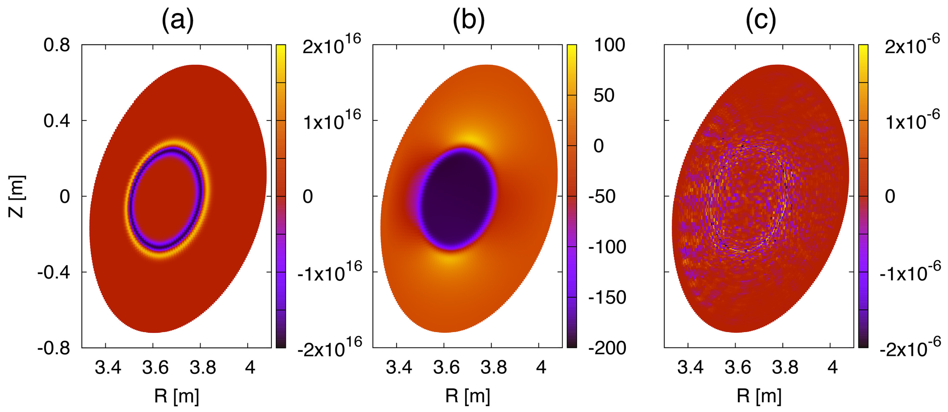
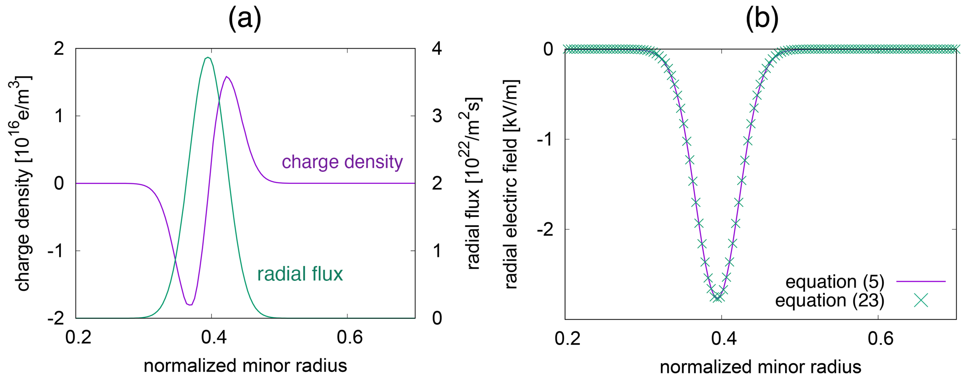
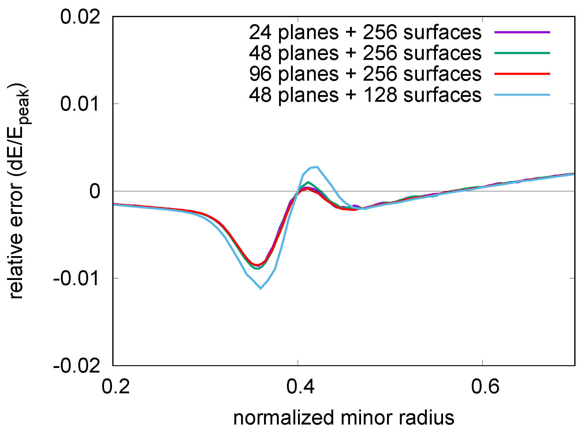
5.3. Field Calculation on Non-Axisymmetric Triangular Mesh

Finite difference and finite element calculations in the “field” process are validated by using a model charge density on the triangular mesh. For simplicity, we consider flux surface averaged charge density and resulting radial electric field. The charge density profile is given by a function of normalized minor radius $\rho$,

$$\begin{array}{ccc}\hfill q(\rho )& =& q_0(\rho +\delta \rho )(V(\rho )/V(\rho +\delta \rho ))-q_0(\rho ),\hfill \end{array}$$

(21)

$$\begin{array}{ccc}\hfill q_0(\rho )& =& {10}^{17}[e/m^3]\exp (-{((\rho -{\rho }_0)/{\rho }_L)}^2),\hfill \end{array}$$

(22)

where $\delta \rho =7.8\times {10}^{-3}$, ${\rho }_0=0.4$, and ${\rho }_L=0.04$. e stands for the elementary charge. $V(\rho )$ is the total volume occupied by the triangle nodes on a flux surface with a normalized minor radius. This profile corresponds to the outward displacement of a uniform charge density on the flux surface. Constant number density $n=3.04\times {10}^{19}({\mathrm{m}}^{-3})$ is assumed. $\delta \rho$, ${\rho }_0$, and ${\rho }_L$ are the displacement, initial position, and width of the charge population, respectively. Figure 11a shows the charge density on the poloidal cross section with $\varphi =1/18(2\pi /10)$. We choose a preconditioned Conjugate Gradient iterative method to solve the linear equations of the finite element Poisson solver with PETSc library. Geometric algebraic multigrid method is used as the preconditioner. Figure 11b shows the obtained electrostatic potential profile. The accuracy of the solution is obtained by evaluating the residual $R\left[\mathsf{\Phi }\right]=\nabla ·((n{m}_i/|B^2|)\nabla \mathsf{\Phi })+q(\rho )$ (see Equation (5)). Figure 11c shows the difference between left hand side (LHS) and right hand side (RHS) terms in the Poisson equation with respect to the basis function in the finite element solver. The color indicates the difference normalized to the maximum value of LHS at the position of each basis function. One can see that the residual error is limited within the order of ${10}^{-6}$ in this case.

The electric field is estimated by the finite difference of the electrostatic potential. This includes finite difference calculation on the triangular mesh and along the magnetic field line in the toroidal direction. Radial component of the electric field from flux-averaged electrostatic can be alternatively estimated by the one-dimensional radial Ampere’s law,

$$\begin{array}{c}\hfill \langle \frac{c^2}{v_A^2}{|\nabla \rho |}^2|\rangle {ϵ}_0\frac{\partial E_r(\rho )}{\partial t}=-q\langle \mathsf{\Gamma }(\rho )\rangle ,\end{array}$$

(23)

where $\mathsf{\Gamma }$ and $v_A$ are flux-averaged radial flux and Alfvén velocity, respectively. $\langle \rangle$ denotes a flux-average operator. A minor term, ${\langle |\nabla \rho |}^2|\rangle {ϵ}_0\partial E_r(\rho )/\partial t$, is neglected in LHS. This equation is analytically equivalent to the gyrokinetic Poisson equation (Equation (5)) for flux-averaged values. The three-dimensional geometry is included in the $\langle c^2/v_A^2|\nabla \rho {|}^2|\rangle$ term. The radial Ampere’s law with the minor term has been employed in neoclassical transport simulations for stellarators using Fortec-3D [40]. For a small $\delta \rho$, radial flux corresponding to the charge density profile in Equation (22) is given by

$$\begin{array}{c}\hfill \mathsf{\Gamma }(\rho )=q_0(\rho +0.5\delta \rho )(V(\rho +0.5\delta \rho )/V(\rho ))\delta \rho /dt.\end{array}$$

(24)

Figure 12a shows profiles of the charge density in Equation (21) and the radial flux in Equation (24). Figure 12b shows the comparison between radial electric field profiles resulting from the Poisson solver and the one-dimensional equation. The former (purple line) is derived by the spatial difference of electrostatic potential, $\mathsf{\Phi }$, which is the solution of the Poisson equation shown in Figure 11b. The latter (green dots) is derived from Equation (23) by substituting the radial flux in the absence of initial electric field. As shown in the figure, these two estimations are in agreement with each other, indicating that the non-axisymmetric configuration is correctly included in three-dimensional derivative calculations of the electrostatic potential.

Figure 13 shows the relative differences between radial electric field profiles resulting from Equations (5) and (23). These are normalized to the peak value of the radial electric field. We perform simulations with different triangle meshes and toroidal resolutions. The triangle meshes have 256 flux surfaces (mesh A: 102,529 mesh vertices per plane) or 128 flux surfaces (mesh B: 25,665 mesh vertices per plane). 24, 48 or 96 poloidal planes are employed per helical field period. Purple, green, red and cyan lines give the differences resulting from mesh A × 24 planes, mesh A × 48 planes, mesh A × 96 planes and mesh B × 48 planes, respectively. In all cases, the differences are comparable to or less than $1\%$ independently of the toroidal resolution. Main differences around $\rho =0.4$ depend on the triangle mesh resolution. This small discrepancy could be caused dominantly by difference between finite difference schemes on the triangle mesh (Equation (5)) and those in the radial direction (Equation (23)).

The finite element solver is also tested in the entire region of the LHD. We could combine two meshes for the core and edge regions with the same triangle nodes along the LCFS. We consider a uniform charge density for the field calculation including the edge region where flux surfaces are not defined, while the charge density profile defined by normalized minor radius is assumed to compared with the field Equation (23) for the core region. Figure 14a shows the electrostatic potential profile obtained for a charge density of ${10}^{15}(e/{\mathrm{m}}^3)$ by assuming constant density and magnetic field, $\left|\mathbf{B}\right|=2(\mathrm{T})$ and $\mathrm{n}={10}^{20}(1/{\mathrm{m}}^3)$. We employ a boundary condition so that the electrostatic potential is equal to zero at the vacuum vessel. The green line in the figure indicates the LCFS where these two meshes are connected to each other. A smooth potential profile is obtained according to the vacuum vessel, independently of the LCFS. The residual error in the Poisson solver is given in Figure 14b. The solver converges within a small residual error ∼$O({10}^{-7})$ in the entire region. These results suggest that the combined triangular mesh works well as a unified mesh in the finite element solver even though mesh generation schemes are quite different in the core and edge regions.

We have illustrated capacity of the triangular mesh to apply to the stellarator edge region satisfying the basic requirements for whole-volume modeling, such as continuity of solutions of the finite element solver and approximate field-following mesh vertices consistent with continuous equilibrium magnetic field. A short fall in the present work is not to solve the gyrokinetic Poisson equation (Equation (5)) in the stellarator edge region with self-consistent charge density from the simulation. This work is on-going and will be reported in the future. Since kinetic plasma dynamics in a stellarator edge region are not understood theoretically, direct comparison with experiments would be needed to validate the simulation code. This is one of the final goals of our work and beyond the scope of this manuscript.

5.4. Benchmark Test on Collisionless Damping of Electric Field Perturbation in LHD

We perform a benchmark calculation of collisionless damping of oscillatory radial electric field perturbations, geodesic acoustic modes (GAMs) [41] in LHD using the field-aligned mesh and Equation (23) [42]. The small initial perturbation of the radial electric field tends to be dissipated into a steady state with a finite residual electric field perturbation [43]. Wavenumber and amplitude of the initial perturbation are $k{\rho }_i=0.7$ and $E_0=1\mathrm{eV}$, respectively. Temperature and density are $1.49\mathrm{keV}$ and $3.04\times {10}^{19}$${\mathrm{m}}^{-3}$, respectively. Simulation results are compared with the results of local analytical theory [44] and another gyrokinetic simulation using GT5D [45]. GT5D is a global Vlasov gyrokinetic code using a flux coordinate system. Figure 15a shows the time evolution of radial electric field averaged on a flux surface with a normalized minor radius $\rho \sim 0.51$ obtained from the present simulation code (blue), GT5D (red) and the analytical theory (green). Collisionless damping of the GAM is observed to have a very similar time scale ∼$10R_{ax}/v_{ti}$ with comparable residual field (∼0.1–0.15$E_0$). Here, $v_{ti}$ is ion thermal velocity. As discussed in [45], the difference between the results of the gyrokinetic simulations and the analytical theory might come from the use of global magnetic field geometry in the simulations. The steady state after the GAM has decayed is sustained by zonal flow along the flux surface (see, Figure 15b) due to $E\times B$ drift motion from the small residual electric field (potential energy is ∼${10}^{-4}$ of the ion thermal energy). Therefore accurate representation of flux surface structures in the unstructured mesh is necessary to demonstrate the steady state.

6. Conclusions and Discussions

A gyrokinetic particle-in-cell simulation code for whole-volume modeling of stellarators has been developed by extending XGC, which was originally developed for tokamaks. The following features are newly implemented to deal with non-axisymmetric geometries and stochastic field line structure in the edge region:

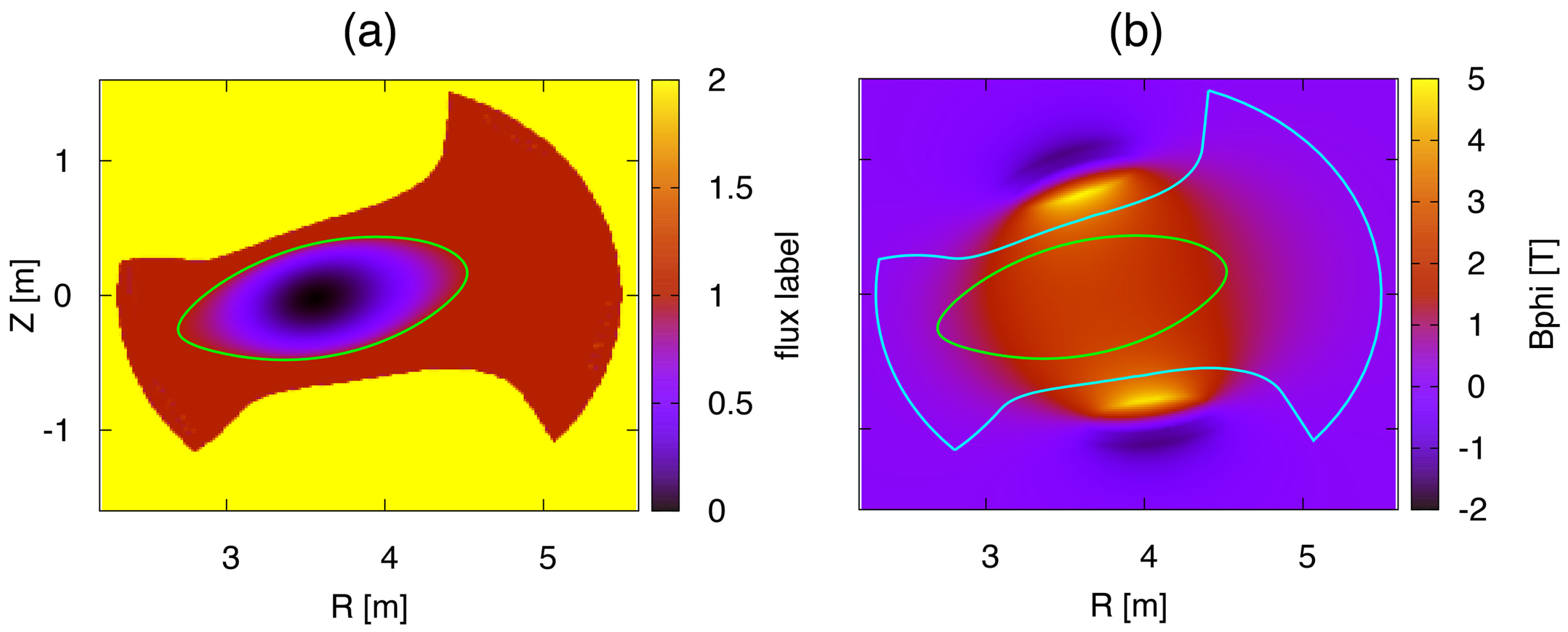
• The magnetic field profiles in the core region are defined by three-dimensional VMEC equilibrium data. The equilibrium data are discretized in the cylindrical coordinate. Three-dimensional spline interpolation is used to obtain magnetic field values at an arbitrary position.
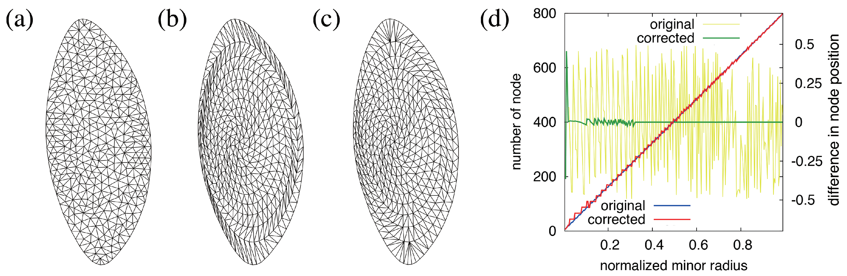
• Non-axisymmetric triangular meshes are generated in the flux coordinate so as to include flux surface structures and follow field lines. Triangular unstructured meshes are employed to define perturbed values such as electrostatic field, charge density, and other plasma fluid moments on planes of constant toroidal angle. The field-aligned mesh is useful to reduce numerical dissipation in particle-mesh interpolation and to enhance numerical efficiency in the field solve.
• The VMEC equilibria are smoothly extended to the edge region of LHD using a virtual casing method. The edge magnetic field is estimated from the surface current of the core region as well as the external coils. The magnetic field in the core region is identical to the VMEC equilibrium, and therefore compatible to the triangular mesh in the core region.
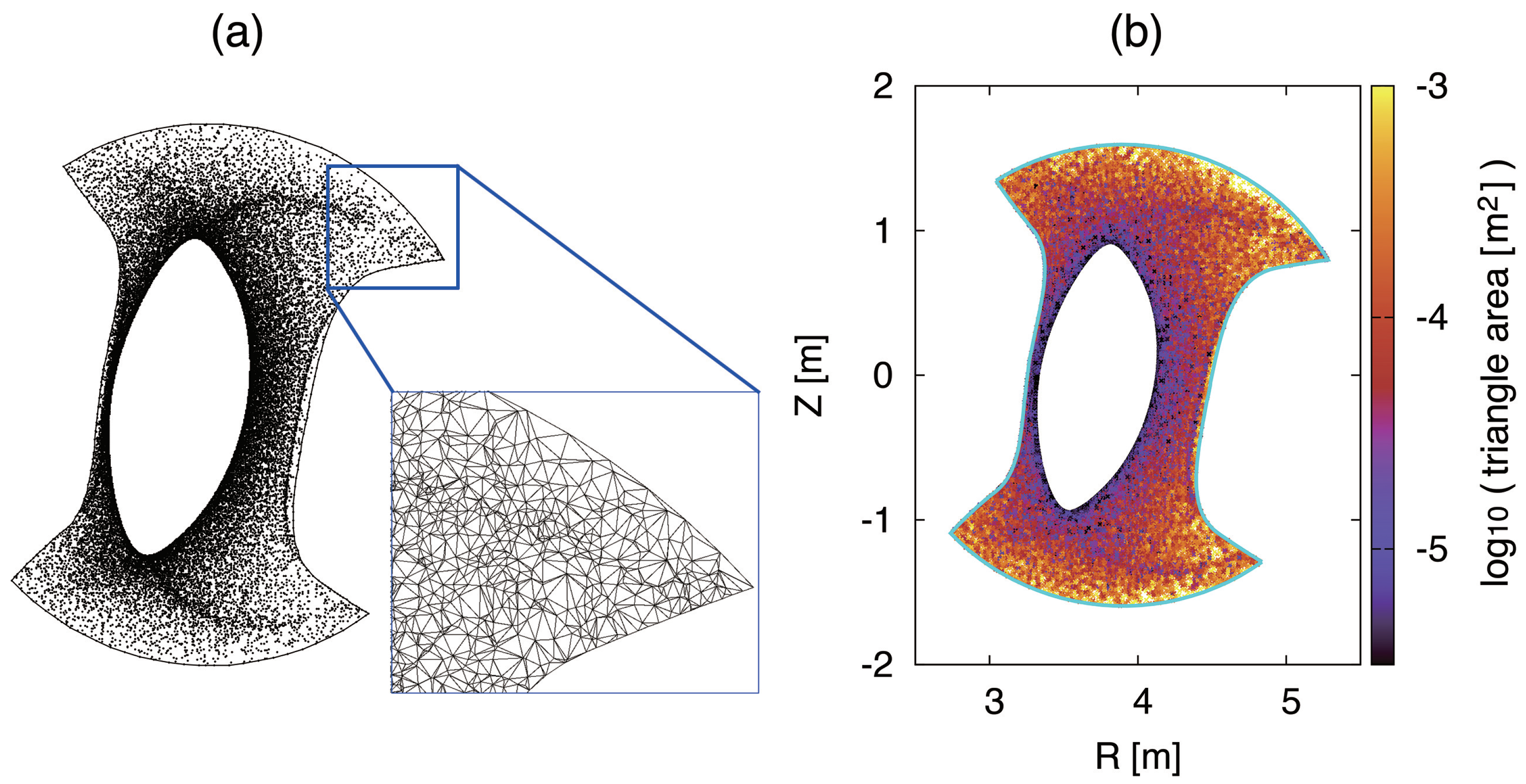
• Field-aligned triangular mesh in the edge region is generated by numerical field line tracing in the extended equilibrium. The generated mesh is automatically refined in the stochastic region and divertor legs. The mesh can relate plasma dynamics to global field line structure through the particle-mesh interpolation.

Benchmark tests for the implemented schemes are performed for each calculation step, “push”, “gather”, “scatter”, and “field”:

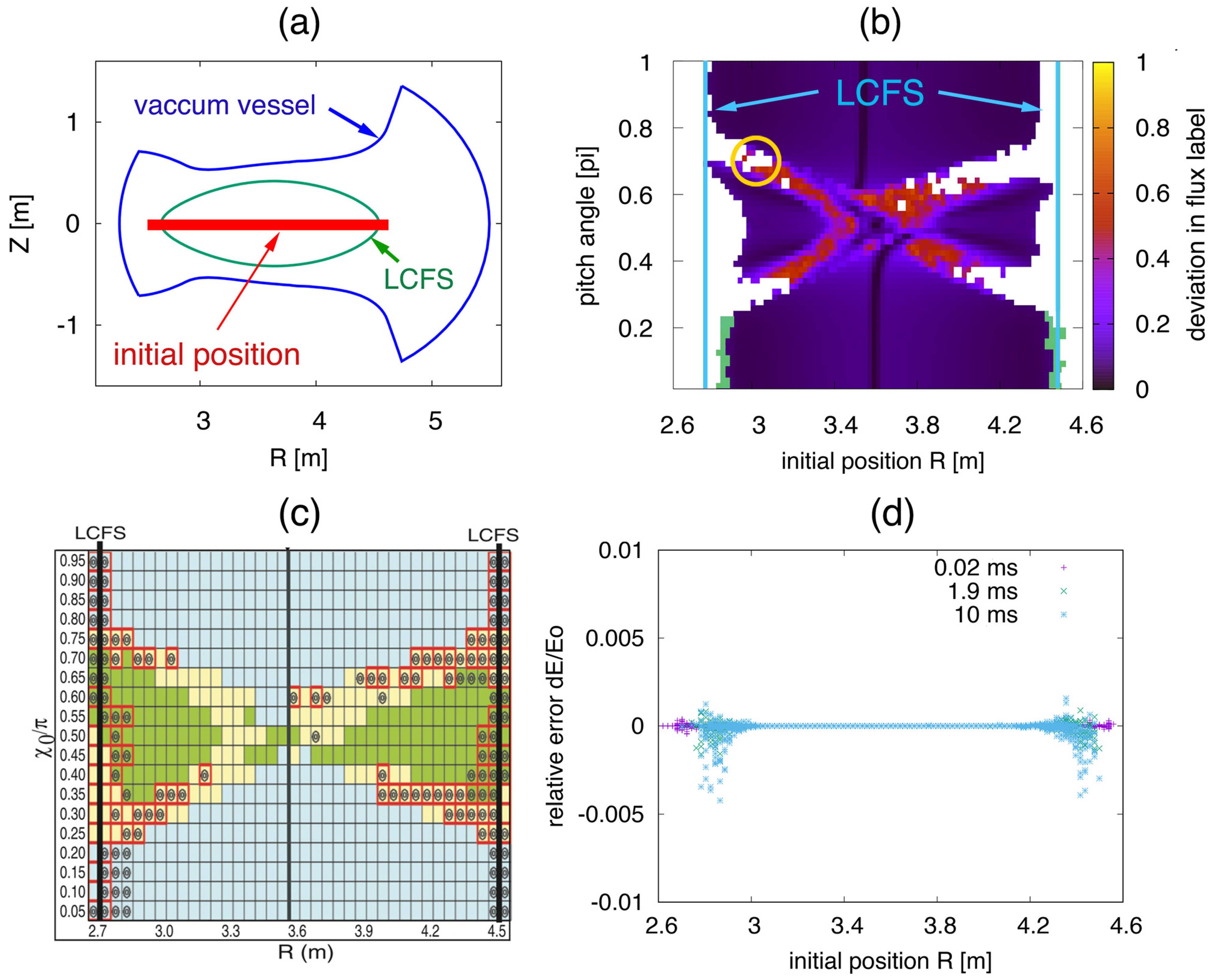
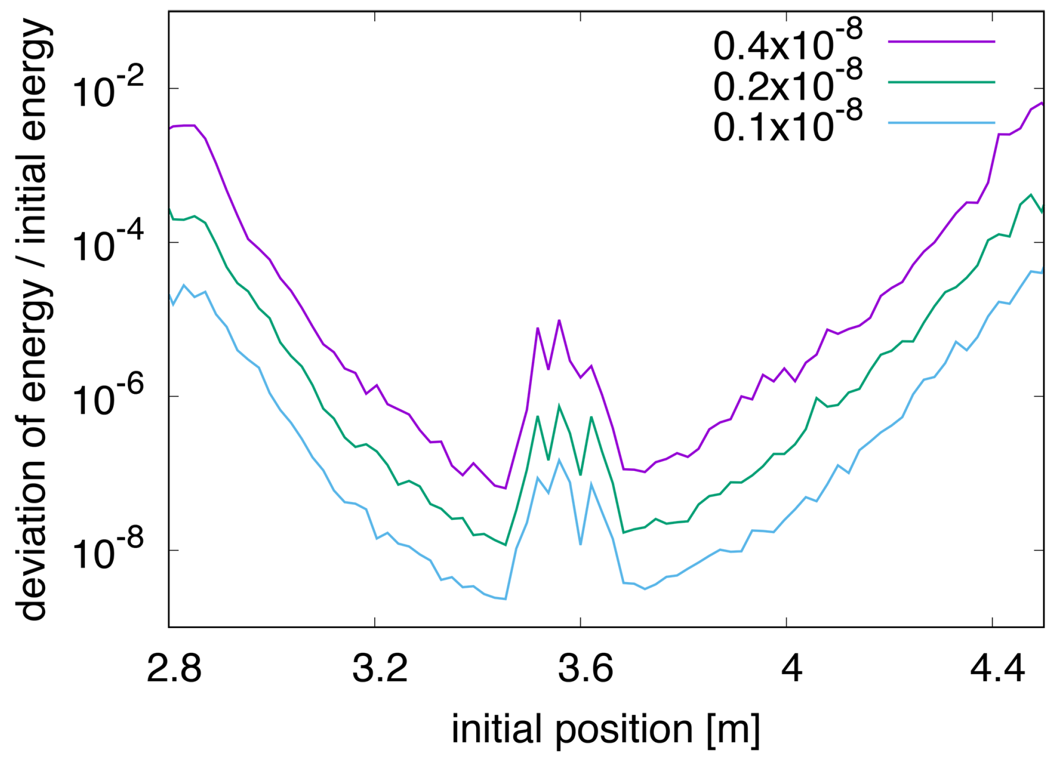
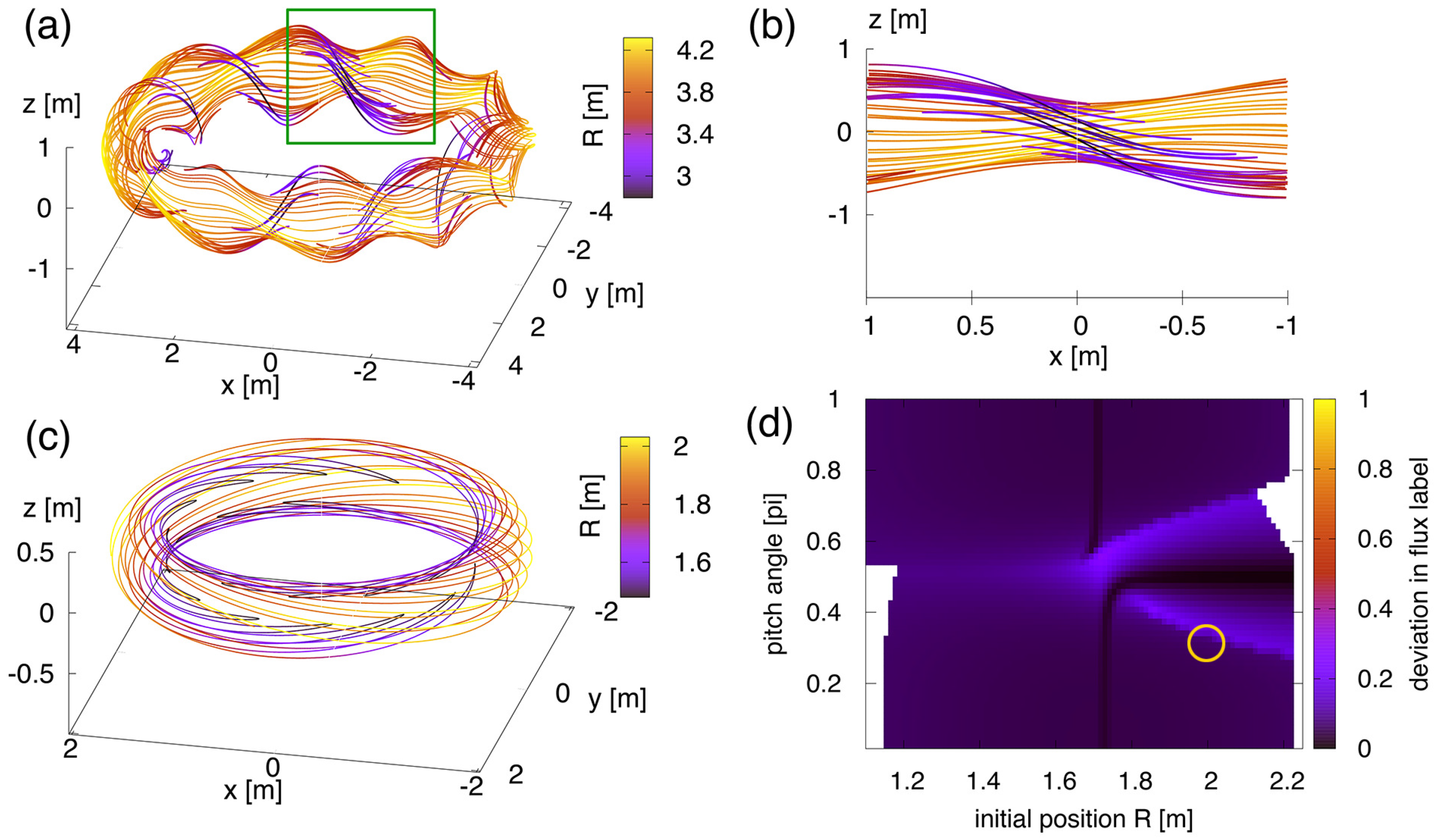
• For the “push” step, particle orbits are calculated in the extended VMEC equilibrium. The relationship between particle loss at the vessel boundary and initial condition (position and pitch angle) is in good agreement with a previous simulation study using a HINT equilibrium. This agreement indicates that the “push” process using three-dimensional spline interpolation can trace particle orbits accurately in the extended VMEC equilibrium.
• For the “field” step, the finite-element Poisson solver is applied to a model charge density profile on the triangular mesh. We confirm that the Poisson solver converges within a small residual level. The flux-surface averaged electrostatic potential evaluated from the alternative equation (radial Ampere’s law) is almost indistinguishable from that obtained from the finite-element gyrokinetic Poission equation. The finite element Poisson solver also converges on the unified triangular mesh including the core and the edge regions to obtain a smooth solution independently of the interface of the two meshes at the last closed flux surface.
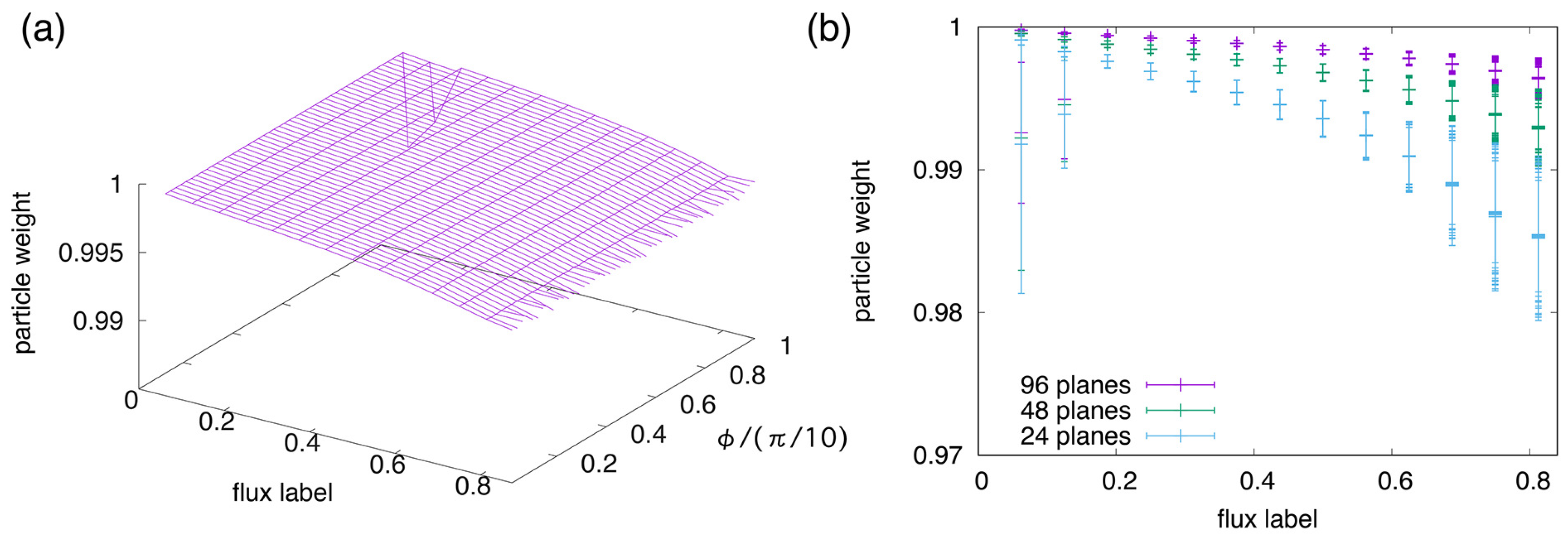
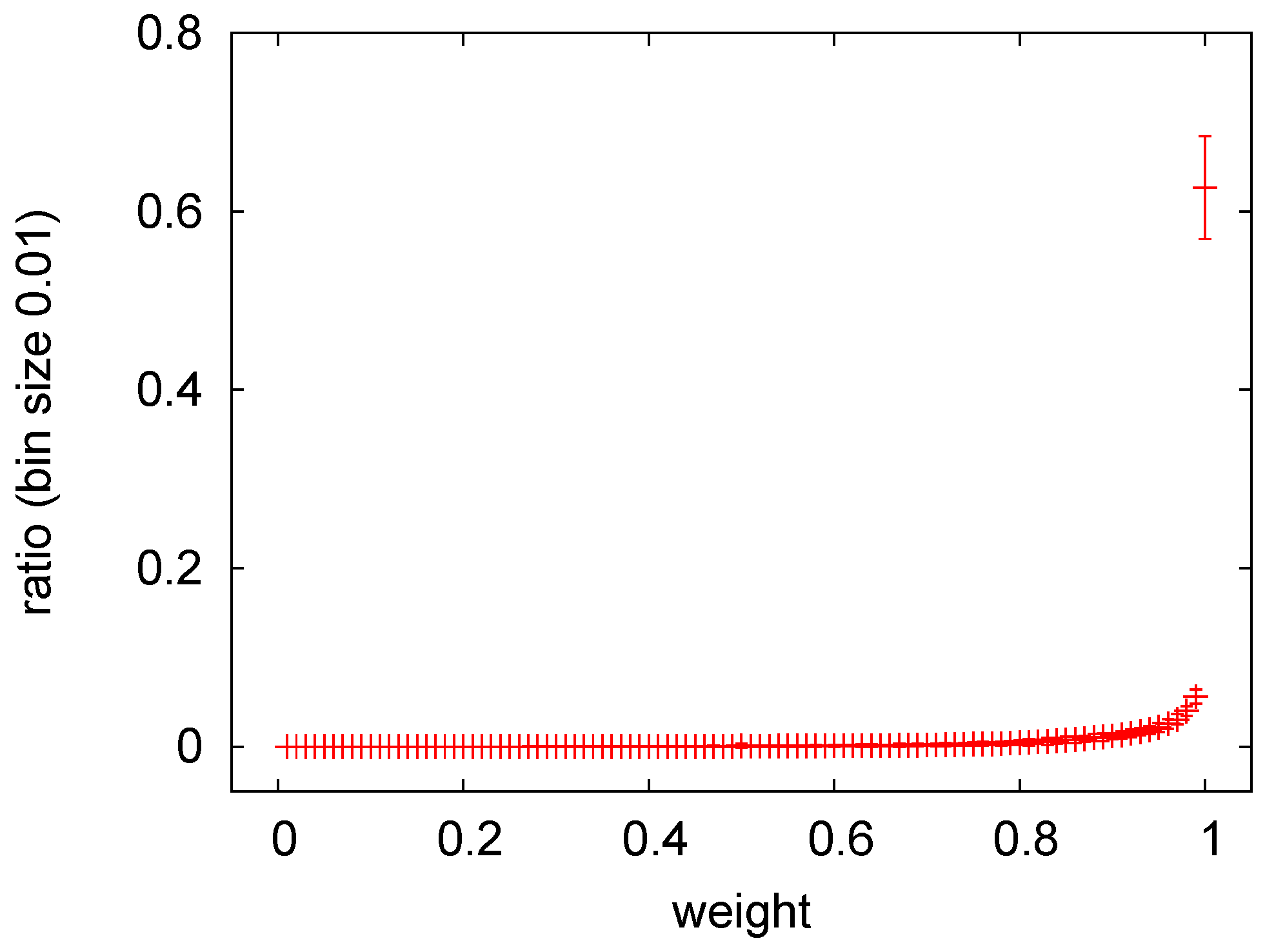
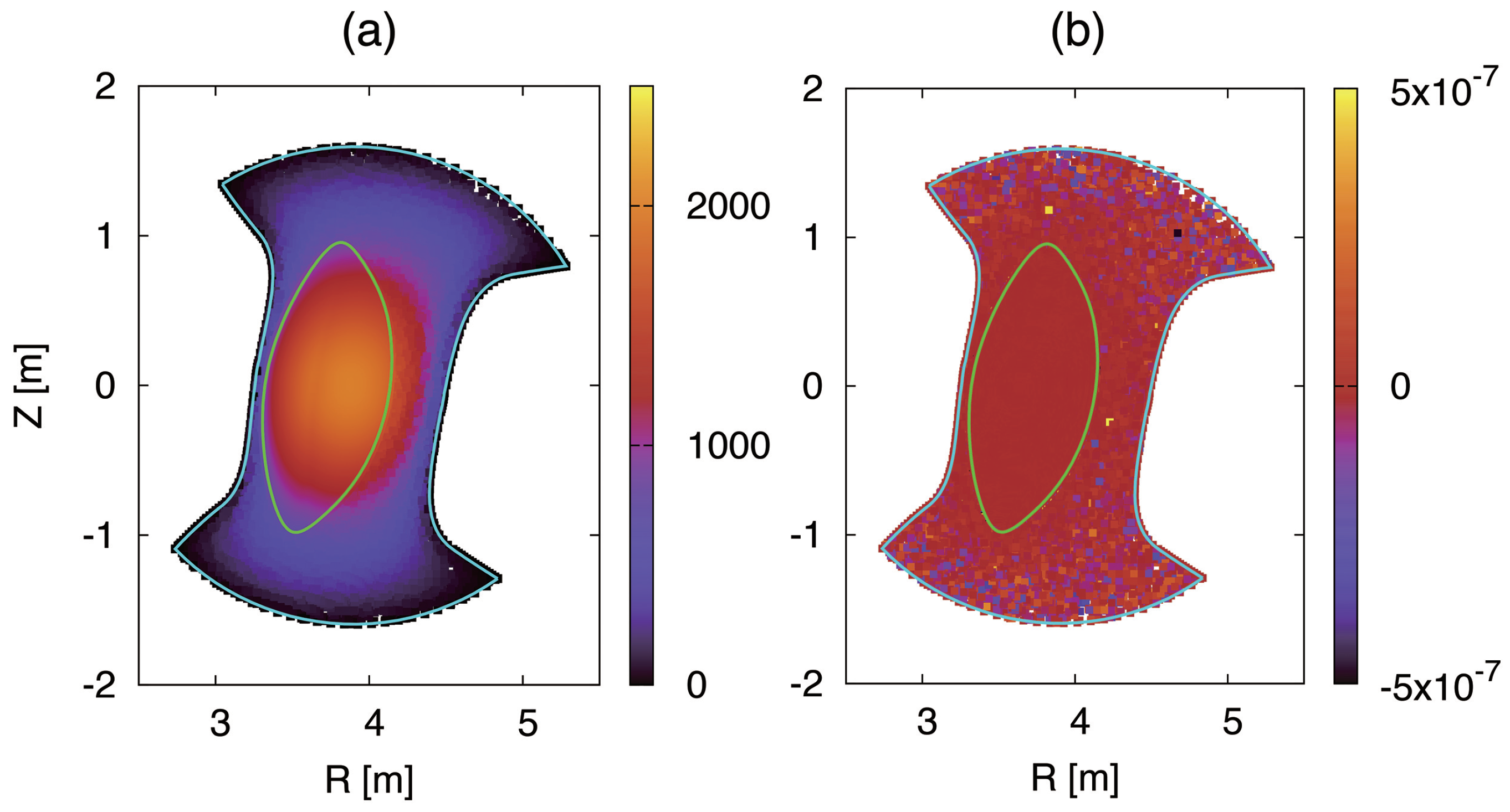
• The particle-mesh interpolation in “gather” and “scatter” processes is applied to a marker particle on the triangular mesh. The field-following interpolation in these procedures is observed to be confined within a certain number of triangle vertices. The particle weight is recovered by gathering the scattered weight without numerical dissipation related to the field following interpolation.

We have presented separate benchmark tests between the single-particle and the field calculations using equilibrium data for LHD. The developed code successfully demonstrates collisionless damping of geodesic acoustic modes and steady states with residual zonal flow in LHD [42]. In this benchmark test, we have considered only flux averaged plasma dynamics relevant to fundamental neoclassical transport phenomena. We will apply the extended XGC code to turbulent transport phenomena and demonstrate linear growth of ion temperature gradient instability [46] in the next step [47].

References

1. Federici, G.; Skinner, C.H.; Brooks, J.N.; Coad, J.P.; Grisolia, C.; Haasz, A.A.; Hassanein, A.; Philipps, V.; Pitcher, C.S.; Roth, J.; et al. Plasma-material interactions in current tokamaks and their implications for next step fusion reactors. Nucl. Fusion 2001, 41, 1967–2137. [Google Scholar] [CrossRef]
2. Wagner, F.; Becker, G.; Behringer, K.; Campbell, D.; Eberhagen, A.; Engelhardt, W.; Fussmann, G.; Gehre, O.; Gernhardt, J.; Gierke, G.; et al. Regime of Improved Confinement and High Beta in Neutral-Beam-Heated Divertor Discharges of the ASDEX Tokamak. Phys. Rev. Lett. 1982, 49, 1408–1412. [Google Scholar] [CrossRef]
3. Kim, E.J.; Diamond, P.H. Zonal Flows and Transient Dynamics of the L-H Transition. Phys. Rev. Lett. 2003, 90, 185006. [Google Scholar] [CrossRef] [PubMed]
4. Loarte, A.; Saibene, G.; Sartori, R.; Riccardo, V.; Andrew, R.; Paley, J.; Fundamenski, W.; Eich, T.; Herrmann, A.; Pautasso, G.; et al. Transient heat loads in current fusion experiments, extrapolation to ITER and consequences for its operation. Phys. Scr. 2007, 222, 115021. [Google Scholar] [CrossRef]
5. Ku, S.; Chang, C.S.; Diamond, P. Full-f gyrokinetic particle simulation of centrally heated global ITG turbulence from magnetic axis to edge pedestal top in a realistic tokamak geometry. Nucl. Fusion 2009, 49, 115021. [Google Scholar] [CrossRef]
6. Chang, C.S.; Ku, S.; Loarte, A.; Parail, V.; Köchl, F.; Romanelli, M.; Maingi, R.; Ahn, J.-W.; Gray, T.; Hughes, J.; et al. Gyrokinetic projection of the divertor heat-flux width from present tokamaks to ITER. Nucl. Fusion 2017, 57, 116023. [Google Scholar] [CrossRef]
7. Ku, S.; Hager, R.; Chang, C.S.; Kwon, J.M.; Parker, S.E. A new hybrid-Lagrangian numerical scheme for gyrokinetic simulation of tokamak edge plasma. J. Comput. Phys. 2016, 315, 467–475. [Google Scholar] [CrossRef]
8. Yoon, E.S.; Chang, C.S. A Fokker-Planck-Landau collision equation solver on two-dimensional velocity grid and its application to particle-in-cell simulation. Phys. Plasmas 2014, 21, 032503. [Google Scholar] [CrossRef]
9. Hager, R.; Yoon, E.S.; Ku, S.; D’Azevedo, E.F.; Worley, P.H.; Chang, C.S. A fully non-linear multi-species Fokker-Planck-Landau collision operator for simulation of fusion plasma. J. Comput. Phys. 2016, 315, 644–660. [Google Scholar] [CrossRef]
10. Zhang, F.; Hager, R.; Ku, S.; Chang, C.S.; Jardin, S.C.; Ferraro, N.M. Mesh generation for confined fusion plasma simulation. Eng. Comput. 2016, 32, 285–293. [Google Scholar] [CrossRef]
11. PETSc: Portable, Extensible Toolkit for Scientific Computation. Available online: https://www.mcs.anl.gov/petsc/ (accessed on 9 May 2019).
12. Spitzer, L. The stellarator concept. Phys. Fluids 1958, 1, 253–264. [Google Scholar] [CrossRef]
13. “XGC” DOE CODE 12570. Available online: https://www.osti.gov/doecode/biblio/12570-xgc (accessed on 9 May 2019).
14. XGC0. Available online: https://epsi.pppl.gov/computing/xgc-0 (accessed on 9 May 2019).
15. XGCa. Available online: https://epsi.pppl.gov/computing/xgca (accessed on 9 May 2019).
16. XGC1. Available online: https://epsi.pppl.gov/computing/xgc-1 (accessed on 9 May 2019).
17. Ku, S.; Chang, C.S.; Hager, R.; Churchill, R.M.; Tynan, G.R.; Cziegler, I.; Greenwald, M.; Hughes, J.; Parker, S.E.; Adams, M.F.; et al. A fast low-to-high confinement mode bifurcation dynamics in the boundary-plasma gyrokinetic code XGC. Phys. Plasmas 2018, 25, 056107. [Google Scholar] [CrossRef]
18. D’Azevedo, E.; Stephen Abbott, S.; Koskela, T.; Worley, P.; Ku, S.; Ethier, S.; Yoon, E.; Shephard, M.; Hager, R.; Lang, J.; et al. Chapter 24. The Fusion Code XGC: Enabling Kinetic Study of Multiscale Edge Turbulent Transport in ITER”. In Exascale Scientific Applications: Scalability and Performance Portability; CRC Press: Boca Raton, FL, USA, 2017. [Google Scholar]
19. Ohyabu, N.; Watanabe, T.; Ji, H.; Akao, H.; Ono, T.; Kawamura, T.; Yamazaki, K.; Akaishi, K.; Inoue, N.; Komori, A. The Large Helical Device (LHD) helical divertor. Nucl. Fusion 1994, 34, 387–399. [Google Scholar] [CrossRef]
20. Toi, K.; Watanabe, F.; Ohdachi, S.; Morita, S.; Gao, X.; Narihara, K.; Sakakibara, S.; Tanaka, K.; Tokuzawa, T.; Urano, H.; et al. L-H Transition and Edge Transport Barrier Formation on LHD. Fusion Sci. Technol. 2010, 58, 61–69. [Google Scholar] [CrossRef]
21. Lao, L.L.; John, H.S.; Stambaugh, R.D.; Kellman, A.G.; Pfeiffer, W. Reconstruction of current profile parameters and plasma shapes in tokamaks. Nucl. Fusion 1985, 25, 1611–1622. [Google Scholar] [CrossRef]
22. Hirshman, S.P.; Whitson, J.C. Steepest-descent moment method for three-dimensional magnetohydrodynamic equilibria. Phys. Fluids 1983, 26, 3353–3568. [Google Scholar] [CrossRef]
23. Lazerson, S.A. The virtual-casing principle for 3D toroidal systems. Plasma Phys. Control. Fusion 2012, 54, 12202. [Google Scholar] [CrossRef]
24. Yamada, H.; The LHD experiment Group. Overview of results from the Large Helical Device. Nucl. Fusion 2011, 51, 094021. [Google Scholar] [CrossRef]
25. Adams, M.F.; Ku, S.; Worley, P.H.; D’ Azevedo, E.; Cummings, J.C.; Chang, C.S. Scaling to 150K cores: Recent algorithm and performance engineering developments enabling XGC1 to run at scale. J. Phys. Conf. Ser. 2009, 180, 012036. [Google Scholar] [CrossRef]
26. Hahm, T.S. Nonlinear gyrokinetic equations for tokamak microturbulence. Phys. Fluids 1988, 31, 2670–2673. [Google Scholar] [CrossRef]
27. Lee, W. Gyrokinetic particle simulation model. J. Comput. Phys. 1987, 72, 243–269. [Google Scholar] [CrossRef]
28. PSPLINE: Princeton Spline and Hermite Cubic Interpolation Routines. Available online: https://w3.pppl.gov/ntcc/PSPLINE/ (accessed on 9 May 2019).
29. Hariri, F.; Ottaviani, M. A flux-coordinate independent field-aligned approach to plasma turbulence simulations. Comput. Phys. Commun. 2013, 184, 2419–2429. [Google Scholar] [CrossRef]
30. Lee, W. Gyrokinetic approach in particle simulation. Phys. Fluids 1983, 26, 556–562. [Google Scholar] [CrossRef]
31. Birdsall, C.K.; Langdon, A.B. Plasma Physics via Computer Simulation; The Adam Hilger Series on Plasma Physics; Taylor and Francis: New York, NY, USA, 1985. [Google Scholar]
32. Sugama, H. Modern gyrokinetic formulation of collisional and turbulent transport in toroidally rotating plasmas. Rev. Mod. Plasma Phys. 2017, 1, 9. [Google Scholar] [CrossRef]
33. Triangle: A Two-Dimensional Quality Mesh Generator and Delaunay Triangulator. Available online: https://www.cs.cmu.edu/~quake/triangle.html (accessed on 9 May 2019).
34. McMillan, M.; Lazerson, S.A. BEAMS3D Neutral Beam Injection Model. Plasma Phys. Control. Fusion 2014, 56, 095019. [Google Scholar] [CrossRef]
35. Spong, D.A.; Hirshman, S.P.; Berry, L.A.; Lyon, L.F.; Fowler, R.H.; Strickler, D.J.; Cole, M.J.; Nelson, B.N.; Williamson, D.E.; Ware, A.S.; et al. Physics issues of compact drift optimized stellarators. Nucl. Fusion 2001, 41, 711–716. [Google Scholar] [CrossRef]
36. Lazerson, S. “STELLOPT“ DOE CODE 12551. Available online: https://www.osti.gov/doecode/biblio/12551-stellopt (accessed on 9 May 2019).
37. Seki, R.; Matsumoto, Y.; Suzuki, Y.; Watanabe, K.; Itagaki, M.T. Particle Orbit Analysis in the Finite Beta Plasma of the Large Helical Device using Real Coordinates. Plasma Fusion Res. 2008, 3, 016. [Google Scholar] [CrossRef]
38. Suzuki, Y.; Nakajima, N.; Watanabe, K.; Nakanura, Y.; Hayashi, T. Development and application of HINT2 to helical system plasmas. Nucl. Fusion 2006, 46, L19. [Google Scholar] [CrossRef]
39. Egedal, J. Drift orbit topology of fast ions in tokamaks. Nucl. Fusion 2000, 40, 1597. [Google Scholar] [CrossRef]
40. Satake, S.; Okamoto, N.; Nakajima, N.; Sugama, H.; Yokoyama, M.; Beidler, C.D. Non-local neoclassical transport simulation of geodesic acoustic mode. Nucl. Fusion 2005, 45, 1362–1368. [Google Scholar] [CrossRef]
41. Winsor, N.; Johnson, J.; Dawson, J. Geodesic Acoustic Waves in Hydromagnetic Systems. Phys. Fluids 1968, 11, 2448–2450. [Google Scholar] [CrossRef]
42. Moritaka, T.; Hager, R.; Cole, M.D.J.; Laserzon, S.; Satake, S.; Chang, C.S.; Ku, S.; Matsuoka, S.; Ishiguro, S. Gyrokinetic Modelling with an Extended Magnetic Equilibrium Including the Edge Region of Large Helical Device. In Proceedings of the 27th IAEA Fusion Energy Conference, Gandhinagar, India, 22–27 October 2018. [Google Scholar]
43. Rosenbluth, M.N.; Hinton, F.L. Poloidal Flow Driven by Ion-Temperature-Gradient Turbulence in Tokamaks. Phys. Rev. Lett. 1998, 80, 724–727. [Google Scholar] [CrossRef]
44. Sugama, H.; Watanabe, T.-H. Collisionless damping of zonal flows in helical systems. Phys. Plasmas 2005, 13, 012501. [Google Scholar] [CrossRef]
45. Matsuoka, S.; Idomura, Y.; Satake, S. Neoclassical transport benchmark of global full-f gyrokinetic simulation in stellarator configurations. Phys. Plasmas 2018, 25, 022510. [Google Scholar] [CrossRef]
46. Horton, W. Drift waves and transport. Rev. Mod. Phys. 1999, 71, 735–778. [Google Scholar] [CrossRef]
47. Cole, M.D.J.; Moritaka, T.; Chang, C.S.; Hager, R.; Ku, S.-H.; Lazerson, S. Confinement in Stellarators with the Global Gyrokinetic Code XGC. In Proceedings of the 27th IAEA Fusion Energy Conference, Gandhinagar, India, 22–27 October 2018. [Google Scholar]
Figure 1. Schematic view of particle-mesh interpolation. (a) Triangular mesh in the ( j + 1 )/2-th cross section. The field-following projected position of a particle at X j m and the corresponding nearest vertices X j n d are given by red and green points in the top panel, respectively. Blue points indicate triangle vertices at which the particle weight is scattered when combining field-following projection (red arrow) and gyro-averaging (green circles). These are scattered to (b) j-th and (c) ( j + 1 )-th cross sections along the field lines (blue points) and distributed onto the triangle nodes on these cross sections (red points). In the gather process, physical quantities on these nodes may be distributed to a wider area surrounded by the red line on the half-integer cross section as shown in the bottom of panel (a).
Plasma 02 00014 g001
Figure 2. Examples of triangular mesh in the core region of the Large Helical Device (LHD). The resolution is reduced to show mesh structures clearly. (a) Fully unstructured mesh; (b) Field-aligned triangular mesh; (c) Field-aligned mesh after triangle shape correction; (d) Number of nodes along the flux surface as a function of normalized minor radius (red). Difference of poloidal angle between the nodes on the 1st poloidal cross section and the positions projected from the nodes on ( k m a x ) -th poloidal cross sections along field lines (yellow for the original mesh and green for the corrected mesh). Smaller difference means higher accuracy of the field-line following interpolation.
Plasma 02 00014 g002
Figure 3. Spatial profile of (a) flux label and (b) magnetic field B ϕ on the poloidal cross section ϕ = 16 / 36 × π / 10 used for three-dimensional spline interpolation. Green and blue lines indicate the last closed flux surface and the vacuum vessel boundary, respectively. The value outside the last closed flux surface in panel (a) corresponds to the vessel boundary.
Plasma 02 00014 g003
Figure 4. (a) Triangle nodes and elements (bounded area) in the edge region obtained from numerical field line tracing. (b) Triangle areas ( m 2 ) in each triangular mesh.
Plasma 02 00014 g004
Figure 5. (a) Initial positions of particles on the poloidal cross section at ϕ = ( 2 π / 10 ) / 2 . (b) Result of the particle tracing benchmark at t = 10.0 ( ms ) . Color coded plot indicates deviation in flux label along the particle orbits as a function of the initial condition, position R (m) and pitch angle. White and green parts represents the lost particles that reach the material boundary and the re-entered particles. Cyan vertical lines indicate the positions of the last closed flux surface (LCFS) on the horizontal axis. The yellow circle indicates initial condition of the particle in Figure 6a,b. (c) Results of another particle tracing calculation [37]. Reprinted from R. Seki, et al., Plasma and Fusion Research, 3, 016 (2008) with permission from JSPF. (d) Deviation of particle energy at t = 0.02 ms (purple), t = 1.9 ms (green), and t = 10.0 ms (blue) as a function of the initial position.
Plasma 02 00014 g005
Figure 6. Deviation of particle energy as a function of the initial position obtained using different time step size. The deviation is averaged over the initial pitch angle and normalized to the initial particle energy, 100 [keV].
Plasma 02 00014 g006
Figure 7. (a) Particle orbit with chaotic motion in LHD. (b) Particle orbit in the green box in panel (a). (c) Typical particle orbit in a circular tokamak. (d) Deviation in flux label along the particle orbits in a circular tokamak as a function of the initial condition, position in R and pitch angle. White parts stand for initial conditions of particles that escape outside LCFS.
Plasma 02 00014 g007
Figure 8. Spatial profiles of particle weight scattered/gathered on two different types of unstructured mesh: (a) fully unstructured mesh and (b) mesh with field-aligned triangle nodes. The green bar is the original particle weight (=1). The orange and red bars are the particle weight scattered on integer and half-integer poloidal cross sections, respectively. (c) Particle weight gathered from triangle nodes after the scatter process estimated for randomly placed particles.
Plasma 02 00014 g008
Figure 9. (a) Particle weight after the gather process as a function of toroidal angle and flux label. The weights are averaged in flux label bins. The bin size is 1 / 16 . (b) Particle weights obtained with 96 (purple), 48 (green) and 24 (blue) poloidal cross sections. The weights are averaged in flux label bins. The error bars stand for standard deviation of particle weight in the bins.
Plasma 02 00014 g009
Figure 10. Statistics of particle weight after the scatter/gather process in the edge region. Weight bin size is 0.01. Error bar indicates standard deviation of the ratio on poloidal cross sections.
Plasma 02 00014 g010
Figure 11. (a) Spatial profile of flux-averaged charge density (e/m 3 ) substituted to the Poisson equation. (b) Electrostatic potential profile (V) as a solution of the Poisson equation using finite element method. (c) Relative error between right hand side and left hand side terms in the converged solution.
Plasma 02 00014 g011
Figure 12. (a) Flux-averaged charge density (purple) and corresponding radial flux (green) evaluated in the field equations. (b) Radial electric field profile resulting from two-dimensional Poisson equation, Equation (5) (purple line) and the one-dimensional equation, Equation (23) (green crosses).
Plasma 02 00014 g012
Figure 13. Difference between radial electric field profiles obtained with Equations (5) and (23) normalized to the peak electric field. Purple, green, red and cyan lines denote the results using mesh A × 24 planes, mesh A × 48 planes, mesh A × 96 planes and mesh B × 48 planes, respectively.
Plasma 02 00014 g013
Figure 14. (a) Potential profile obtained from finite element Poisson solver on the unified mesh for a constant charge density. (b) Residual level of the relative error in the Poisson solver.
Plasma 02 00014 g014
Figure 15. (a) Time evolution of radial electric field resulting from the present simulation code (blue), another gyrokinetic code, GT5D (red), and the analytical theory (green). (b) Schematic picture of flux surface and zonal flow in LHD.
Plasma 02 00014 g015