The Effect of Magnetic Field Strength and Geometry on the Deposition Rate and Ionized Flux Fraction in the HiPIMS Discharge

Abstract

We explored the effect of magnetic field strength $\left|\mathbf{B}\right|$ and geometry (degree of balancing) on the deposition rate and ionized flux fraction $F_{\mathrm{flux}}$ in dc magnetron sputtering (dcMS) and high power impulse magnetron sputtering (HiPIMS) when depositing titanium. The HiPIMS discharge was run in two different operating modes. The first one we refer to as “fixed voltage mode” where the cathode voltage was kept fixed at 625 V while the pulse repetition frequency was varied to achieve the desired time average power (300 W). The second mode we refer to as “fixed peak current mode” and was carried out by adjusting the cathode voltage to maintain a fixed peak discharge current and by varying the frequency to achieve the same average power. Our results show that the dcMS deposition rate was weakly sensitive to variations in the magnetic field while the deposition rate during HiPIMS operated in fixed voltage mode changed from 30% to 90% of the dcMS deposition rate as $\left|\mathbf{B}\right|$ decreased. In contrast, when operating the HiPIMS discharge in fixed peak current mode, the deposition rate increased only slightly with decreasing $\left|\mathbf{B}\right|$. In fixed voltage mode, for weaker $\left|\mathbf{B}\right|$, the higher was the deposition rate, the lower was the $F_{\mathrm{flux}}$. In the fixed peak current mode, both deposition rate and $F_{\mathrm{flux}}$ increased with decreasing $\left|\mathbf{B}\right|$. Deposition rate uniformity measurements illustrated that the dcMS deposition uniformity was rather insensitive to changes in $\left|\mathbf{B}\right|$ while both HiPIMS operating modes were highly sensitive. The HiPIMS deposition rate uniformity could be 10% lower or up to 10% higher than the dcMS deposition rate uniformity depending on $\left|\mathbf{B}\right|$ and in particular the magnetic field topology. We related the measured quantities, the deposition rate and ionized flux fraction, to the ionization probability ${\alpha }_{\mathrm{t}}$ and the back attraction probability of the sputtered species ${\beta }_{\mathrm{t}}$. We showed that the fraction of the ions of the sputtered material that escape back attraction increased by 30% when $\left|\mathbf{B}\right|$ was reduced during operation in fixed peak current mode while the ionization probability of the sputtered species increased with increasing $\left|\mathbf{B}\right|$, due to increased discharge current, when operating in fixed voltage mode.

1. Introduction

Conventional dc magnetron sputtering (dcMS) suffers from a low degree of ionization of the sputtered material. High power impulse magnetron sputtering (HiPIMS) has emerged as a promising alternative, providing a highly ionized material flux, while being compatible with conventional magnetron sputtering deposition systems [1]. HiPIMS operation is characterized by a pulsed high peak power in the range of several kW/cm${}^2$ and consequently a high plasma density of up to ${10}^{19}$ m${}^{-3}$ in the cathode target vicinity, which is up to three orders of magnitude higher than in dcMS [2]. Such discharge conditions result in a significant increase of ionization of the sputtered neutrals, where ionized flux fractions $F_{\mathrm{flux}}$ well above 50% have been reported [3,4,5]. However, a high ionized flux fraction commonly comes at a cost of lower deposition rate, which has thus far limited the use of HiPIMS in industry [1,6].

Several reports demonstrate the lower deposition rate in (mainly non-reactive) HiPIMS when compared to dcMS operated at the same average power [1,7]. The seminal work of Kouznetsov et al. [3] reports up to 80% lower deposition rate for HiPIMS than for dcMS. Samuelsson et al. [8] compared the deposition rates from eight metal targets (Ti, Cr, Zr, Al, Cu, Ta, Pt, and Ag) in pure Ar for both dcMS and HiPIMS discharges applying the same average power. They observed HiPIMS deposition rates in the range of 30–85% of the dcMS rates depending on target material.

There are several suggestions on the cause of the lower deposition rate observed in HiPIMS deposition [2,7]. It is generally agreed on by the scientific community that back attraction of ionized sputtered material to the target, quantified as back attraction probability ${\beta }_{\mathrm{t}}$, plays a major role in the reduction of the amount of sputtered particles reaching the substrate [9]. The reason is that atoms ionized in the cathode region are likely to be back-attracted to the target due to strong electric fields in the presheath and extended presheath [10,11]. Spatial measurements of the plasma potential in HiPIMS discharges [11,12,13,14] have shown that there commonly is a potential uphill, from the cathode sheath edge and reaching far outside the ionization region (several cm), that can vary in the range 7–100 V.

Several attempts have been made to increase the deposition rate in HiPIMS. This includes varying the pulse length [15,16,17], varying the magnetic field strength $\left|\mathbf{B}\right|$ [13,18,19], modifying the magnetic field geometry [20,21,22], adding an external magnetic field in the target vicinity [23], chopping the pulse into a train of shorter pulses [24,25], and increasing the target temperature [26]. Several of these reports propose that modifying the magnetic field, using either permanent magnets or electromagnets [13,18,19,27], is one of the most promising approaches. For example, Čapek et al. [18] showed that lowering $\left|\mathbf{B}\right|$ in HiPIMS can have a profound effect on increasing the deposition rate. Using spacers of different thicknesses behind the cathode to reduce $\left|\mathbf{B}\right|$ at the target (and also increasing the average discharge voltages to achieve nominally similar power levels), the deposition rate of Nb was increased by roughly a factor of 5. Similarly, Mishra et al. [13] found a six-fold increase in the deposition rate of Ti by weakening $\left|\mathbf{B}\right|$ by 33%. Bradley et al. [19] reported on a deposition rate increase by a factor of 2 for a Ti target when the magnetic field strength at the target was reduced by 45%. In addition, while weakening $\left|\mathbf{B}\right|$ by 82% a factor of 2.6 higher deposition rate was observed while depositing vanadium films by HiPIMS, although for the weaker magnetic field the films exhibited significantly higher surface roughness and were not as dense [28].

There have also been a few attempts to modify the magnetic field geometry in order to improve the deposition rate. This includes the work of Yu et al. [20], who used a 36 cm diameter magnetron with a spiral-shaped magnet pack assembly to increase the plasma uniformity in the substrate vicinity and to improve target utilization. More recently, Raman et al. [22] modified the magnetic field topology of a HiPIMS discharge, which increased the deposition rate by up to a factor of 2 [22,29]. In the cited studies, the modified magnet pack had a strong magnetic field region over three concentric race track regions (referred to as a TriPack magnetron assembly), but the magnetic field strength fell off more steeply than for a conventional magnet pack when moving away from the target surface. However, those designs encounter some difficulties when scaled down to a smaller cathode size.

The combined effect of weakening $\left|\mathbf{B}\right|$, the correlation between the deposition rate increase and the lower ionized flux fraction to the substrate, is still poorly understood. One reason is that most HiPIMS studies on ionization indeed quantify $F_{\mathrm{flux}}$, but have so far not focused on changing the magnetic field strength/topology. For example, Lundin et al. [5] explored the ionized flux fraction for Al, C and Ti targets using a gridless ion meter. For a Ti target, they found an increase in the ionized flux fraction from roughly 20% to 68% with increased peak discharge current density in the range of 0.7–2.5 A/cm${}^2$. These values are in line with the work of Poolcharuansin et al. [30] (30–50%) and Kubart et al. [4] (20–60%) for current densities in the range 1–2.5 A/cm${}^2$. Another reason is that the studies on $F_{\mathrm{flux}}$ did not in parallel systematically investigate the deposition rate (or the change thereof). The exception is the study of Raman et al. [31], who, in addition to the previously discussed deposition rate study, also estimated the ionized flux fraction during HiPIMS operation using conventional and TriPack magnetrons. They recorded an ionized flux fraction of Cu of approximately 5% for the conventional magnetron and 16% utilizing the TriPack magnetron assembly, which indicates that optimization of the magnetic field can in fact result in increased deposition rate as well as increased ionized flux fraction.

In the present study, we therefore systematically investigated the relationships among $\left|\mathbf{B}\right|$, the magnetic field geometry (level of balancing), the deposition rate, and the ionized flux fraction during HiPIMS and dcMS operation. Such an approach enabled us to study the combined effects of HiPIMS pulse parameters and magnetic configurations. In the analysis, we used the well known materials pathway model [9,32] to assess both the ionization probability ${\alpha }_{\mathrm{t}}$ and the back attraction probability ${\beta }_{\mathrm{t}}$ from the experimental data. Finally, we attempted to explain our observations based on the physics behind the transport of charged particles in these devices.

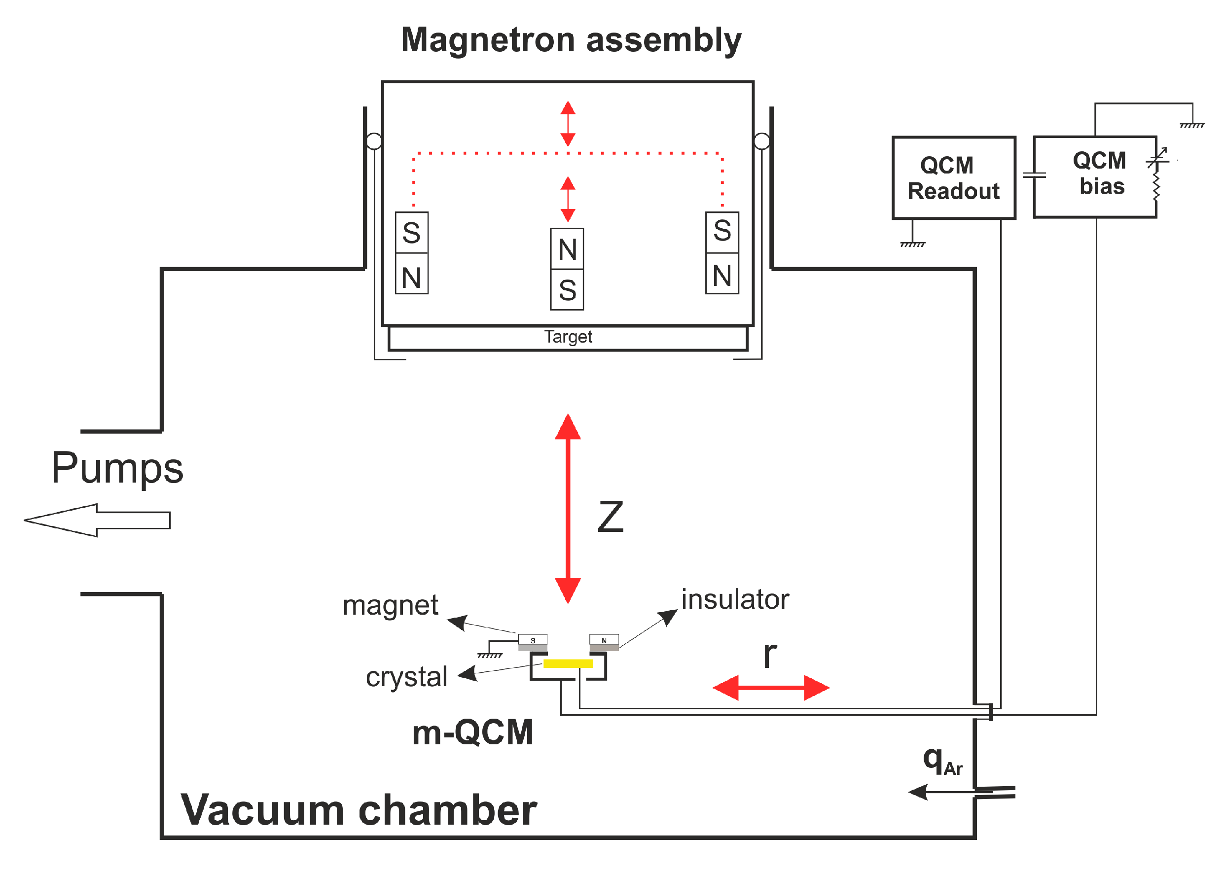
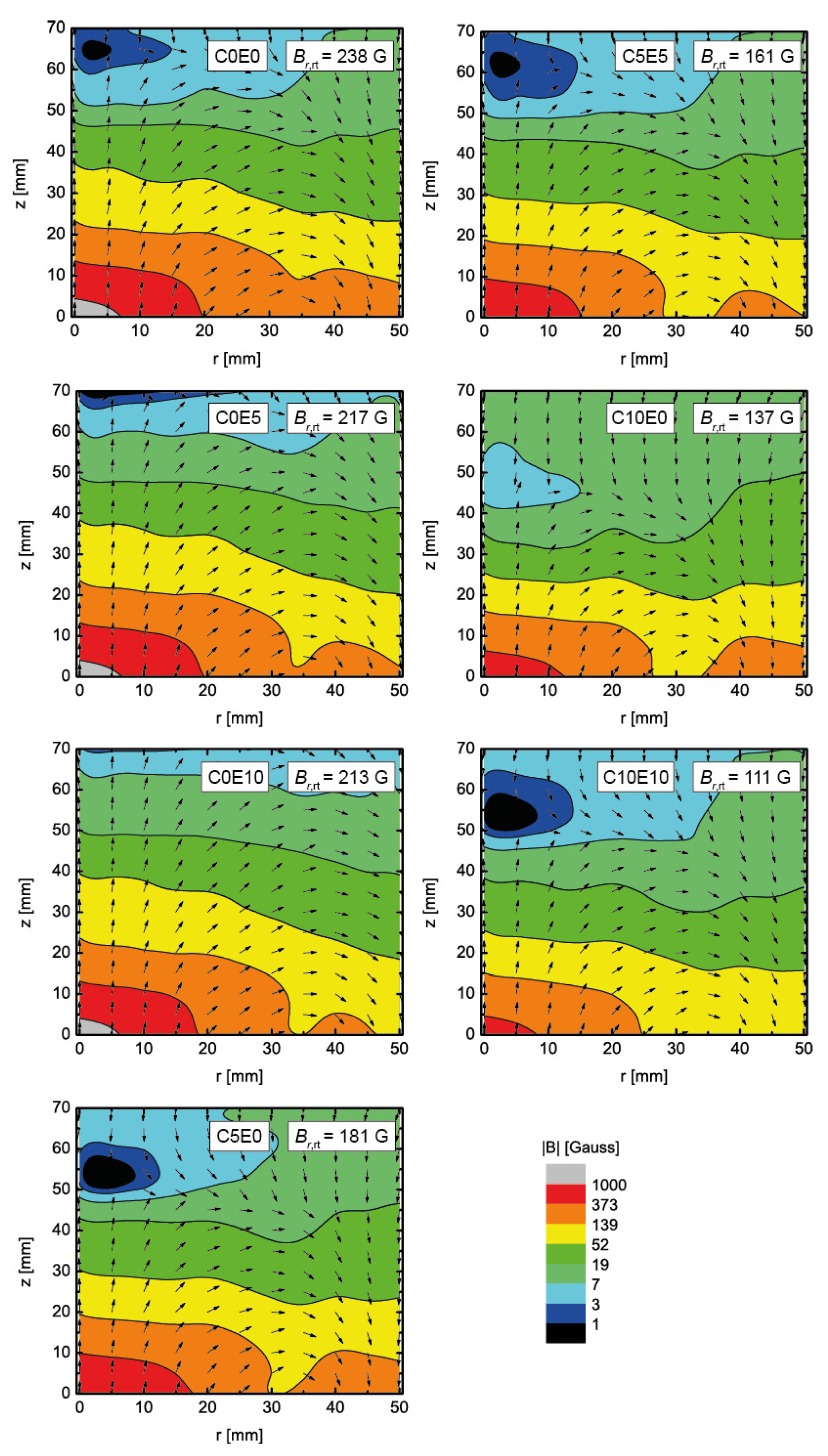
2. Materials and Methods

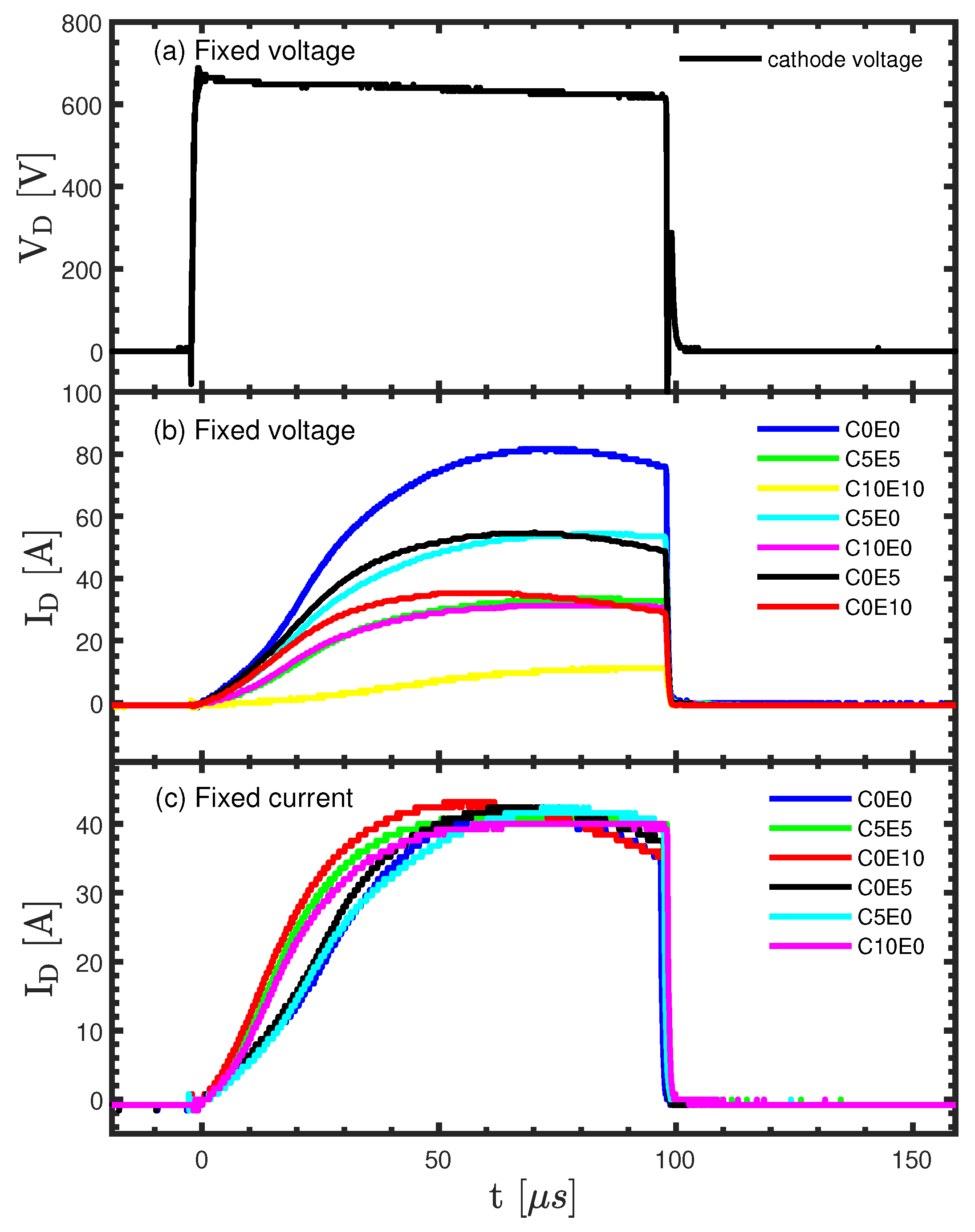
All experiments were carried out in a custom-built cylindrical vacuum chamber (height 50 cm and diameter 45 cm) made of stainless steel. A base pressure of $4\times {10}^{-6}$ Pa was achieved using a turbo molecular pump backed by a roughing pump. The working gas pressure was adjusted to 1 Pa by injecting 50 sccm Ar into the chamber and adjusting a butterfly valve located between chamber and the turbo pump. The deposition system was equipped with a circular 4 inch diameter VTec Magnetron assembly (Gencoa, Liverpool, UK). The magnetron assembly, as well as a probe holder used during measurements, was mounted on movable bellows controlled with millimeter precision, as shown in Figure 1. This made it possible to perform radial as well as axial scans with high precision. The absolute magnetic field strength $\left|\mathbf{B}\right|$ as well as the geometry of the magnetic field (degree of balancing) above the magnetron target was varied by displacing the center magnet (C) and the outer ring magnet at the target edge (E) using two micrometer screws located on the outer side of the magnetron assembly. We refer to each configuration using the displaced distance (in mm) of each magnet from the target backing plate. Thus, the notation C0E0 refers to a magnetron configuration where the center and outer magnets touch the backing plate (zero displacement, i.e., the strongest magnetic field above the target).

In this work, we investigated seven different magnet configurations: C0E0, C5E5 and C10E10, C0E5, C0E10, C5E0, and C10E0. For all of these configurations, the magnetic field above the target was mapped using a Lake Shore 425 Gauss meter (Lake Shore Cryotronics, Westerville, OH, USA) equipped with a Hall probe. The magnetic field distribution above the target for each configuration is shown in Figure 2. Axial symmetry was assumed. For the configurations investigated, it was found that a magnetic null point was always present, which means that all configurations ware categorized as unbalanced type II [33]. The magnetic null was used as a measure of the degree of balancing. The magnetic null point for the different cases was located at 43–74 mm from the target surface above the target center and is given in

Table 1. Discharge operating parameters for the investigated dcMS and HiPIMS discharges in fixed voltage and in fixed peak current modes. The average discharge power was kept at 300 W for all the discharges. For HiPIMS discharges, the pulse length was 100 $\mathsf{\mu }$s while the pulse frequency was varied to maintain a constant averaged power. The absolute magnetic field strength and the degree of balancing was varied by displacing the center magnet (C) and the outer ring magnet at the target edge (E). Each configuration is referred to using the displaced distance (in mm) of each magnet from the target backing plate. In this notation, C0E0 refers to a magnetron configuration where the center and outer magnets touch the backing plate.

	Magnet		dcMS		HiPIMS			HiPIMS			HiPIMS
					Fixed Voltage			Fixed Peak Current			Fixed Peak Current
	${\mathit{B}}_{\mathit{r},\mathbf{rt}}$	${\mathbf{z}}_{\mathbf{null}}$	${\mathit{V}}_{\mathbf{D}}$	${\mathit{I}}_{\mathbf{D}}$	${\mathit{V}}_{\mathbf{D}}$	${\mathit{I}}_{\mathbf{D}\mathbf{,}\mathbf{peak}}$	${\mathit{f}}_{\mathbf{pulse}}$	${\mathit{V}}_{\mathbf{D}}$	${\mathit{I}}_{\mathbf{D},\mathbf{peak}}$	${\mathit{f}}_{\mathbf{pulse}}$	${\mathit{V}}_{\mathbf{D}}$	${\mathit{I}}_{\mathbf{D}\mathbf{,}\mathbf{peak}}$	${\mathit{f}}_{\mathbf{pulse}}$
	[Gauss]	[mm]	[V]	[A]	[V]	[A]	[Hz]	[V]	[A]	[Hz]	[V]	[A]	[Hz]
C0E0	238	66	339	0.885	625	80	54	510	40	143	555	80	60
C0E5	217	70	308	0.974	625	54	76	565	40	123	580	80	56
C0E10	213	74	311	0.964	625	35	115	650	40	111
C5E0	181	53	317	0.946	625	53	80	557	40	129	582	80	58
C5E5	161	59	334	0.926	625	36	97	655	40	97	649	80	295
C10E0	137	43	312	0.961	625	31	134	660	40	99	636	80	295
C10E10	111	52	330	0.909	625	12	450

for each configuration. Note, however, that the case C0E10 was only weakly unbalanced, i.e., close to being balanced ($z_{\mathrm{null}}=74$ mm), whereas C10E0 was the most strongly unbalanced ($z_{\mathrm{null}}=43$ mm). Table 1 also lists the radial component of the magnetic field strength next to the target surface over the race track $|B_{r,\mathrm{rt}}|$. These values were recorded at $z=11$ mm, which was the closest distance that could be probed for the $B_r$ component.

A dc power supply (SR1.5-N-1500, Technix, Créteil, France) and a HiPIMS power supply (HiPSTER 1, Ionautics, Linköping, Sweden) were used to ignite the discharge in dc and HiPIMS modes, respectively. For both cases, an average discharge power was maintained at 300 W. The HiPIMS pulse was always kept at constant length of 100 $\mathsf{\mu }$s and the discharge was regulated in two different ways. The first mode is referred to as fixed voltage mode, and was realized by keeping the cathode voltage fixed at 625 V and varying the pulse frequency to achieve the desired average power. The second mode is referred to as fixed peak current mode and was realized by changing the cathode voltage to maintain the peak discharge current at $I_{\mathrm{D},\mathrm{peak}}$ = 40 A, corresponding to current density $J_{\mathrm{D},\mathrm{peak}}$ = 0.5 A/cm${}^2$ for the ionized flux fraction measurements, and $I_{\mathrm{D},\mathrm{peak}}$ = 80 A and $J_{\mathrm{D},\mathrm{peak}}$ = 1.0 A/cm${}^2$ for the measurements of deposition rate. Again, the pulse frequency was varied to achieve the desired average power. The discharge parameters are summarized in Table 1 for dcMS operation and both operating modes of HiPIMS for all the seven magnet configurations investigated.

We captured the discharge current–voltage ($I_{\mathrm{D}}$–$V_{\mathrm{D}}$) waveforms when operating the HiPIMS discharges at different magnet configurations. Figure 3a depicts the cathode voltage and Figure 3b the discharge current for all seven magnetic field configurations explored when operating in fixed voltage mode. When moving both the central and outer magnets together, $I_{\mathrm{D},\mathrm{peak}}$ changed from 80 A to 36 A to finally 12 A for the C0E0, C5E5 and C10E10 magnet configurations, respectively. Figure 3b shows that $I_{\mathrm{D},\mathrm{peak}}$ occurred before the pulse end using the C0E0 configuration while for two other magnet configurations the discharge current waveforms had an ascending trend over the entire pulse length. The value of $I_{\mathrm{D},\mathrm{peak}}$ was more sensitive to the absolute strength of the magnetic field than to the degree of balancing. The C5E0 and C0E5 configurations gave $I_{\mathrm{D},\mathrm{peak}}$ = 53–54 A and the C10E0 and C0E10 configurations 31–35 A. Figure 3c depicts the discharge current waveforms captured at fixed peak current mode with various magnet configurations. Although $I_{\mathrm{D},\mathrm{peak}}$ was very similar in all cases, the current rise rate was different and as a result the discharge current peaked at different times. Note that different cathode voltages were applied to achieve the same $I_{\mathrm{D},\mathrm{peak}}$ (see Table 1), but the voltage was not correlated to the time of peak current. For example, the C5E5 magnet configuration exhibited sharper current rise than C0E0 while the corresponding cathode voltage was 150 V higher than for the C0E0 magnet. In contrast, looking at discharge current waveforms for the C5E0 and C10E0 magnets showed that using the C5E0 magnet resulted in sharper current rise than the C10E0 magnet, although the corresponding cathode voltage was approximately 100 V lower.

A quartz crystal micro-balance (QCM) with native frequency of 5 MHz and gold coated surface was used to measure the deposition rate. It was mounted on the probe holder shown in Figure 1. By moving the probe holder and/or the magnetron assembly, it was possible to investigate a region defined by $0\le r\le 50$ and $20\le z\le 70$ mm, where r is the radial coordinate parallel to the target surface and z is the axial coordinate perpendicular to the target surface, and $(r,z)=(0,0)$ marks the center of the target surface. The center of the target race track was located at approximately $(r,z)=(30,0)$ mm. In this work, only axial material fluxes were investigated, i.e., mimicking a conventional sputtering setup with a substrate facing the target surface.

The QCM sensor was also used as a main component in the ion meter (or gridless QCM/m-QCM) used for measuring the ionized flux fraction $F_{\mathrm{flux}}$. The device is described in detail in a previous work [4] and is here only summarized. The ion meter can measure either the deposition rate from ions and neutrals or from neutrals only by varying a voltage applied to the biased top QCM electrode, allowing for fast (roughly 1 min) determination of the ionized fraction of material flux to the sensor head. The gridless sensor uses a magnetic field configuration consisting of a ferromagnetic yoke and magnetic pole pieces (cylindrical SmCo magnets with a diameter of 8 mm and a length of 5 mm) placed in front of the sensor. This configuration produces a localized homogeneous magnetic field of about 4000 Gauss, which does not significantly affect the magnetic field of the magnetron assembly [4]. The QCM control unit with the oscillator was connected directly to the crystal electrode. The electrode was either grounded for measurements of both ions and neutrals, or biased to +40 V to collect only the neutrals without positive ions. The dc bias voltage was connected to the QCM collecting electrode through a 1 k$\mathsf{\Omega }$ resistor, to protect the crystal in case of arcing, and the ground of the oscillator and the readout unit were connected to the crystal collecting electrode through a 150 nF capacitor such that dc current was blocked while rf current could flow from the crystal through this capacitor back to the ground of the oscillator and give a readout (see Figure 1). In this configuration, the top crystal electrode could be readily biased without any influence on the QCM operation. The ionized fraction of the metal flux

$$F_{\mathrm{flux}}=\frac{R_{\mathrm{t}}-R_{\mathrm{n}}}{R_{\mathrm{t}}},$$

(1)

was determined from the total mass deposition rate $R_{\mathrm{t}}$ and the mass deposition rate of neutral metal atoms $R_{\mathrm{n}}$, as discussed by Wu et al. [34]. The deposition rates were recorded by manually recording the film thickness at a chosen time on a readout unit connected to the QCM. In addition, we tried to minimize errors due to the QCM crystal heating up during the process by making short measurements (typically less than 120 s). The total error of $F_{\mathrm{flux}}$ was estimated to be up to 15% for a single result mainly based on the accuracy of the mass deposition rate determination. Since the QCM electrode was grounded during the measurement of the total deposition rate, no significant collimation of the ions [35] was expected at this stage due to the low plasma potential, which potentially could introduce additional errors in the measurements. The ion meter was mounted on the probe holder shown in Figure 1 and could thereby map out the same region of interest as the standard QCM. However, due to interference with the plasma discharge, it was not possible to move it closer than $z\ge 30$ mm. In addition, high peak currents in the HiPIMS mode sometimes resulted in strong fluctuations of $(R_{\mathrm{t}}-R_{\mathrm{n}})$, which meant that the HiPIMS series with fixed peak current had to be limited to $I_{\mathrm{D},\mathrm{peak}}$ = 40 A ($J_{\mathrm{D},\mathrm{peak}}$ = 0.5 A/cm${}^2)$ when measuring $F_{\mathrm{flux}}$.

3. Results

The deposition rates as well as the ionized flux fractions for each of the magnetron configurations shown in Figure 2 and listed in Table 1 are presented here. For the deposition rate results, we chose to focus on the data recorded at a typical target-to-substrate distance of $z=70$ mm, which also includes three radial points ($r=0,25,50$ mm) to determine the expected film thickness profile at that axial distance. However, the deposition rate was also recorded closer to the target and comparisons were made where appropriate. Concerning the ionized flux fraction at $z=70$ mm, we only show data recorded above the target center, i.e., $(r,z)=(0,70)$ mm, although all radial positions were used in the analysis. We also show the flux fractions at $(r,z)=(25,30)$ mm due to the interest in comparing with other reports of $F_{\mathrm{flux}}$, which are typically recorded at the outer edge of the ionization region (the dense plasma region) above the target race track. We refer to the region where the substrate is typically located as the diffusion region.

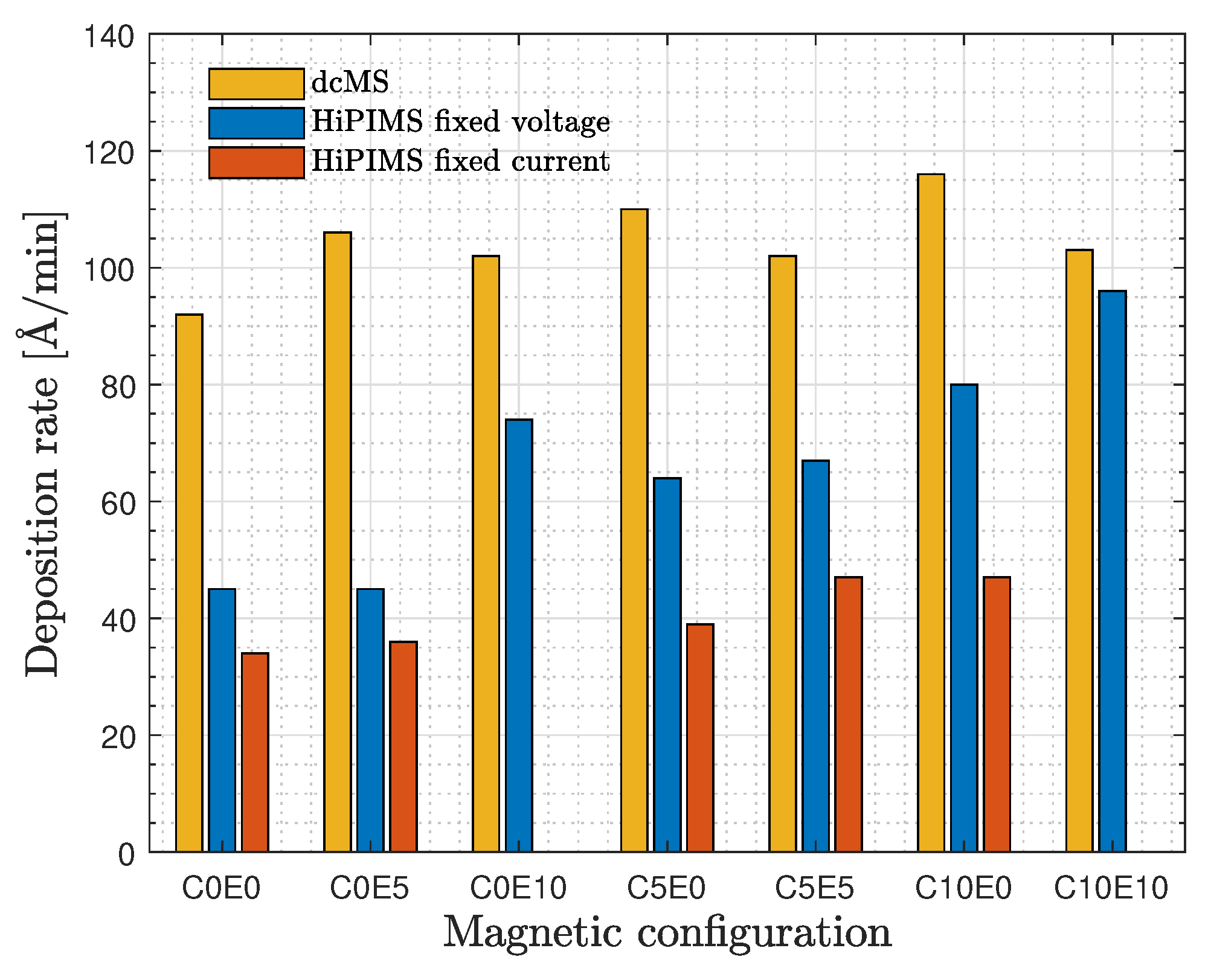
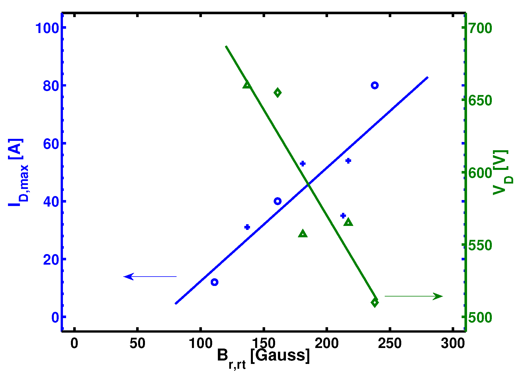
3.1. Deposition Rate

The deposition rates measured above the center of the target ($r=0$ mm) at an axial distance of 70 mm (substrate position) are plotted as a bar chart in Figure 4 for the different discharge types as well as all magnetic configurations investigated. The magnet configurations on the x-axis are ordered from highest $\left|\mathbf{B}\right|$ at the left to the lowest $\left|\mathbf{B}\right|$ on the right. We have here used the recorded $|B_{r,\mathrm{rt}}|$ value above the race track as a measure of $\left|\mathbf{B}\right|$. Overall, the dcMS discharges exhibited the highest deposition rates independent of magnetron configuration, with deposition rates in a rather narrow range (92–116 Å/min). Much larger differences were observed for the HiPIMS discharge operated in the fixed voltage mode, where the deposition rate varied between 45 Å/min and 96 Å/min. However, for the fixed peak discharge current mode, the deposition rate varied between 34 Å/min and 47 Å/min with an increasing trend of 38% larger deposition rate at the weakest $\left|\mathbf{B}\right|$ compared to the strongest $\left|\mathbf{B}\right|$.

Let us start by comparing the three cases C0E0, C5E5, and C10E10, exhibiting the same magnetic topology but approximately a reduction of 63% of the absolute magnetic field strength at the center of the target surface and a reduction of $|B_{r,\mathrm{rt}}|$ by 53% (configurations C0E0 and C10E10). For the dcMS discharges, only small differences were found. The strongest magnetic field (C0E0) showed the lowest deposition rate (92 Å/min) and the weakest magnetic field (C10E10) showed the highest deposition rate (103 Å/min), i.e., a deposition rate increase of 11%. The HiPIMS discharges operated in fixed voltage mode showed a much more pronounced deposition rate dependence on changes in $\left|\mathbf{B}\right|$, where a weaker $\left|\mathbf{B}\right|$ resulted in a considerably higher deposition rate. For example, C0E0 exhibited the lowest deposition rate (45 Å/min) and C10E10 the highest deposition rate (96 Å/min), i.e., a rate increase of 113%. It was also observed that this latter HiPIMS case resulted in a deposition rate, which was around 90% of the dcMS rate, i.e., a significantly higher value than what is commonly reported for HiPIMS, as discussed in the Introduction. In contrast, the HiPIMS discharges operated in fixed peak current mode exhibited smaller changes in the measured deposition rate when $\left|\mathbf{B}\right|$ was varied, as observed when comparing cases C0E0 and C5E5 (no data from C10E10), about 38% increase of the deposition rate when weakening $\left|\mathbf{B}\right|$. In this discharge mode, the HiPIMS deposition rate was around 40% of the dcMS rate for the equivalent magnetron configurations, which was closer to the value of 30% reported by Samuelsson et al. [8].

For completeness, it is also noted that a significant deposition rate increase could be achieved at closer target-to-substrate distances, as expected. The highest deposition rate values, independent of discharge type and magnet configuration, were recorded at the closest axial distance investigated, $z=20$ mm, with on the average, 2.3, 2 and 1.9 times higher values for dcMS, fixed voltage and fixed peak current HiPIMS discharges, respectively, compared to the values measured at $z=70$ mm (results not shown here). In general, similar trends in the deposition rate for the different configurations investigated were observed at all distances from the target. However, the closer was the distance to the target, the larger was the radial variation in the recorded deposition rates, which is generally not desired in thin film deposition.

To address the issue of the expected radial film thickness profile at the substrate position, the relative standard deviation (RSD) of the deposition rate was calculated from recorded deposition rates at three radial points, $r=0,25,50$ mm at $z=70$ mm from the target surface. RSD is a standardized measure of dispersion of a probability distribution or frequency distribution. It is often expressed as a percentage, and is defined as

$$\mathrm{RSD}=100\frac{\sigma }{\mu }$$

(2)

where $\sigma$ is the standard deviation and $\mu$ is the mean of the dataset. The standard deviation of the deposition rates was calculated as the square root of its variance. Overall, we found a weak trend of decreasing RSD with increasing degree of magnetic balancing. This is illustrated in Figure 5, where the magnet configurations on the x-axis are ordered with increasing $z_{\mathrm{null}}$ (increasing degree of magnetic balancing) from left to right (see Table 1).

In addition, the dcMS discharges exhibited the lowest sensitivity to $\left|\mathbf{B}\right|$, as can be seen when comparing the three cases C0E0, C5E5, and C10E10. Note that this does not imply that the coating uniformity was the best since RSD was still rather high. Changing the magnet configuration from weakly to strongly unbalanced configurations (C0E5 to C5E0 and C0E10 to C10E0) barely affected the dcMS deposition rate uniformity, which remained in the range of 16% to 19%.

The deposition rate of a HiPIMS discharge operated in fixed voltage mode exhibited the most uniform deposition rate profile of all cases investigated when using the C5E0 magnetic field geometry with RSD of $12\%$. The C0E5 and C0E10 configurations led to similar RSDs (15%). The lowest uniformity (highest RSD) achieved was observed for C10E0, just below 20%, i.e., similar to the corresponding dcMS value. In the fixed peak current mode, the maximum RSD recorded was 22% for C10E0 and C5E5, while using C0E5 and C5E0 resulted in RSD values of 14% and 16%, respectively. A similar analysis of the fixed voltage HiPIMS mode showed that the highest RSD was 23% when using the C10E10 configuration and the lowest RSD was 12% with the C5E0 configuration. For the strongest $\left|\mathbf{B}\right|$ case C0E0, the deposition rate profile was similar to the dcMS case. However, the RSD values found for the fixed peak current HiPIMS mode were generally higher with RSD of $19\%$ for C0E0 and RSD of $22\%$ for C5E5. Overall, the deposition uniformity was more dependent on the magnetic configuration than the discharge type. Moving closer to the target ($z=20$ mm), the deposition rate became significantly less uniform (about two times higher RSD values) compared to a typical substrate position ($z=70$ mm).

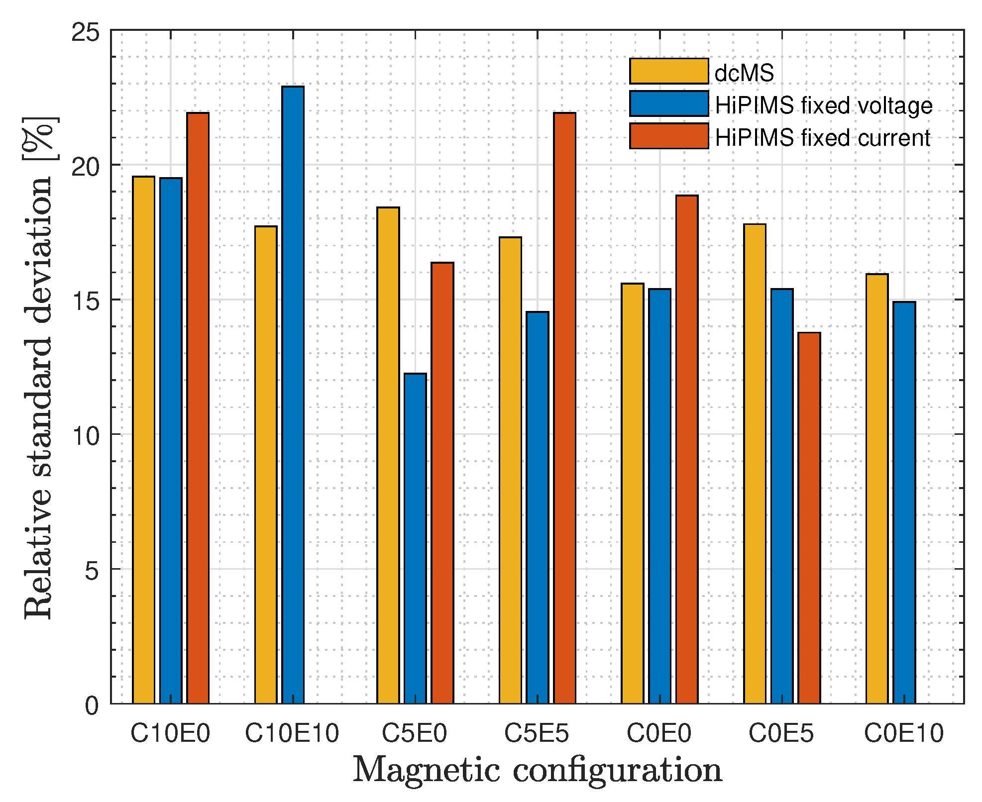
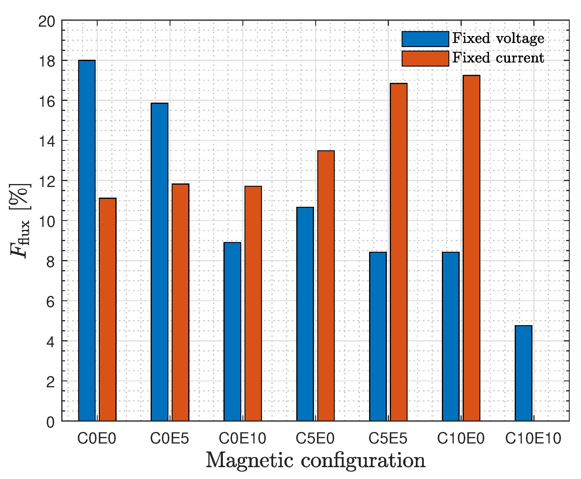
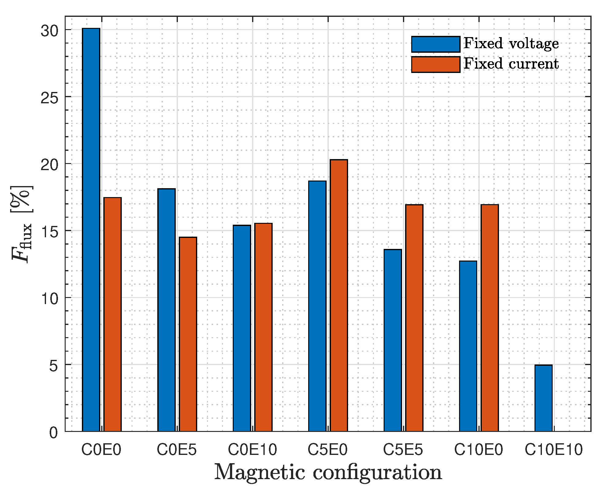
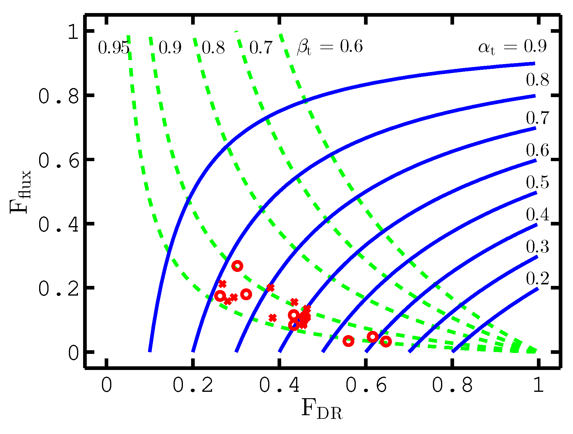
3.2. Ionized Flux Fraction

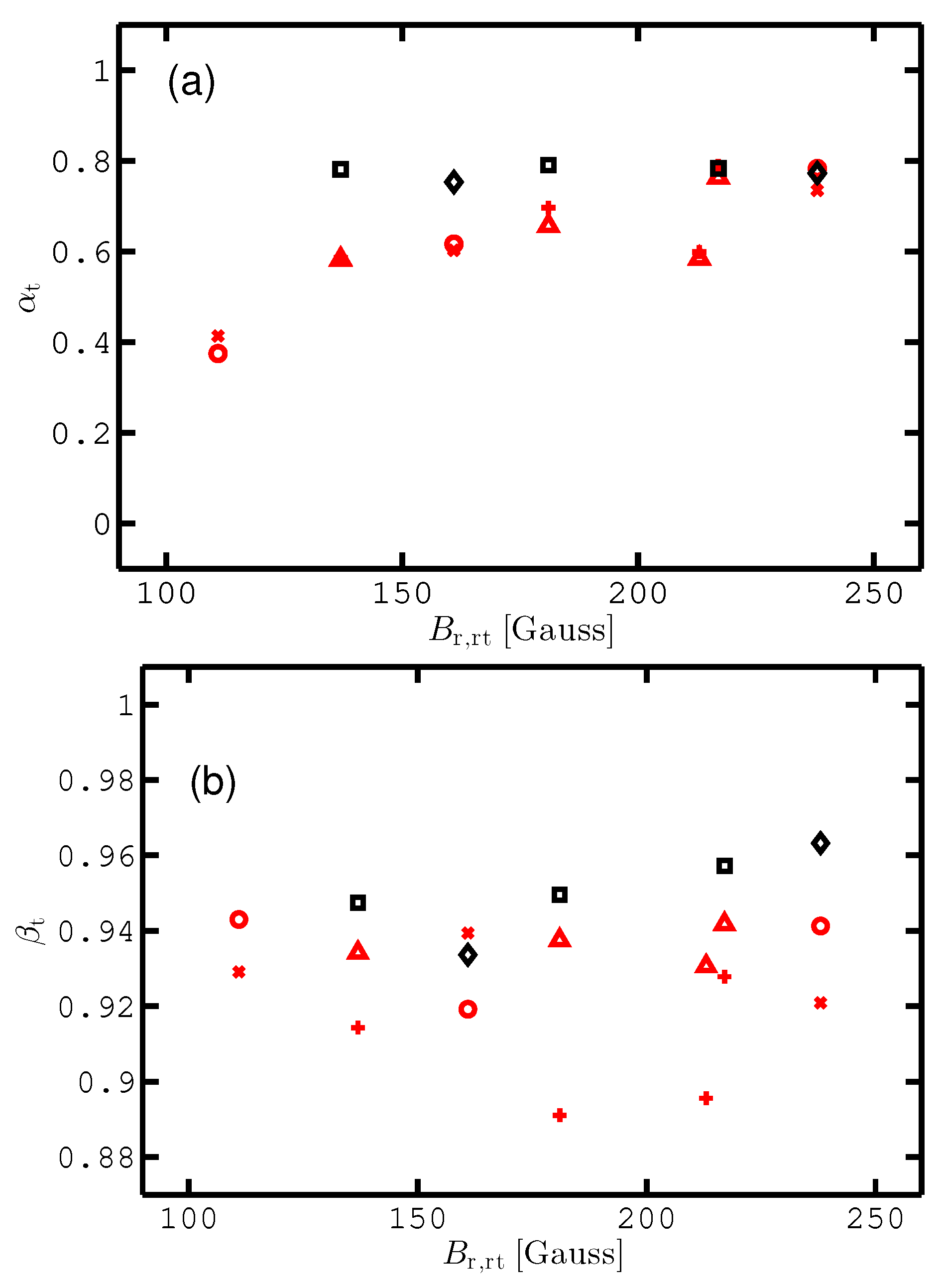
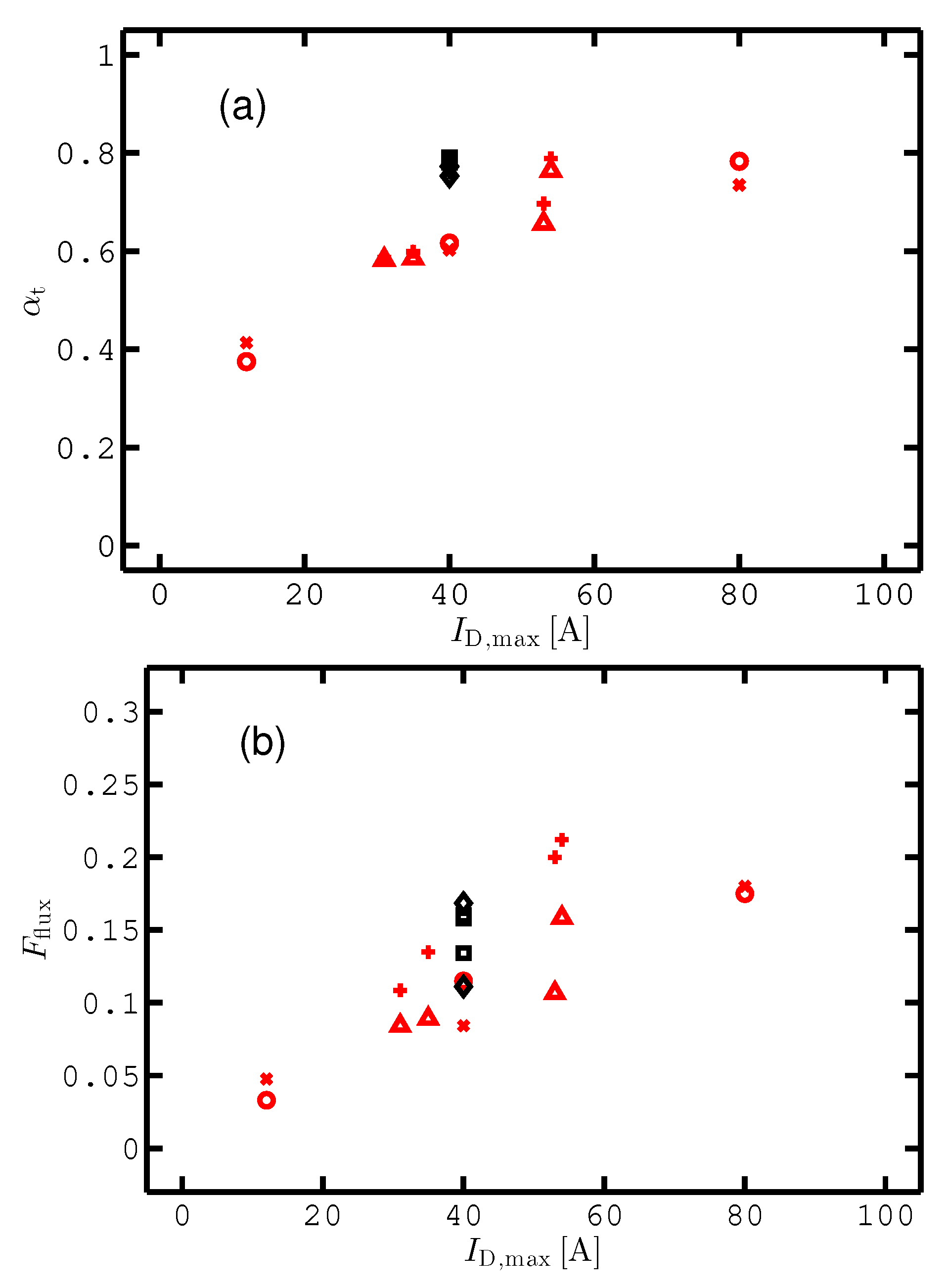
The ionized flux fractions $F_{\mathrm{flux}}$ measured above the center of the target ($r=0$ mm) at an axial distance of $z=70$ mm are plotted as a bar chart in Figure 6 for the two HiPIMS operating modes (fixed voltage and fixed peak current modes) as well as for all magnet configurations investigated. Note that the magnet configurations on the x-axis are now ordered from highest $\left|\mathbf{B}\right|$ at the left to the lowest $\left|\mathbf{B}\right|$ on the right where, again, $|B_{r,\mathrm{rt}}|$ from Table 1 was used as a suitable indicator of $\left|\mathbf{B}\right|$. No dcMS values are presented here, since $F_{\mathrm{flux}}$ was always very close to 0%, i.e., within the margin of error, and thus in line with the results reported by Kubart et al. [4] using the same technique.

Figure 6 shows that the ionized flux fraction decreased with decreasing $\left|\mathbf{B}\right|$ when the HiPIMS discharge was operated in fixed voltage mode. For the HiPIMS discharges operated in fixed voltage mode, significant differences were found when comparing the three cases C0E0, C5E5, and C10E10 (reduced absolute magnetic field strength $\left|\mathbf{B}\right|$, while maintaining the same magnet topology). The strongest magnetic field (C0E0) showed the highest $F_{\mathrm{flux}}$ (18%) and the weakest magnetic field (C10E10) showed the lowest $F_{\mathrm{flux}}$ (4.7%). In the fixed voltage mode, $F_{\mathrm{flux}}$ seemed to decrease with the decreased absolute magnetic field strength $\left|\mathbf{B}\right|$ which is correlated with the peak discharge current presented above in Figure 3. This is analyzed in more detail in the next section. However, the corresponding HiPIMS discharges operated in fixed peak current mode clearly did not exhibit such a behavior. Instead, the ionized flux fraction $F_{\mathrm{flux}}$ increased slightly with decreasing $\left|\mathbf{B}\right|$. The ionized flux fraction increased from 11% to 16.8% when comparing cases C0E0 and C5E5 (no data from C10E10), i.e., by a factor 1.5 when decreasing $\left|\mathbf{B}\right|$.

When focusing on changes in the degree of balancing, i.e., comparing the configuration pairs C0E5/C5E0 and C0E10/C10E0, the following observations could be made. For the HiPIMS discharges operated in fixed voltage mode, it was somewhat surprising that the highest $F_{\mathrm{flux}}$ was recorded for the weakly unbalanced C0E5 configuration (16%), whereas the most strongly unbalanced configuration C10E0 exhibited a much lower value (8.5%), although there was only a small difference compared to C5E0 and C0E10. Any influence on $F_{\mathrm{flux}}$ from the unbalance was masked by the strong influence of the peak discharge current values on $F_{\mathrm{flux}}$. For the HiPIMS discharges operated in fixed peak current mode, the trend observed for $F_{\mathrm{flux}}$ (Figure 6) was somewhat more expected. The more strongly unbalanced cases exhibited higher $F_{\mathrm{flux}}$ with a maximum of 17.2% for C10E0.

In addition, by making radial scans of $F_{\mathrm{flux}}$, we attained radial profiles at $z=70$ mm in the fixed voltage mode (not shown here). In general, only minor differences compared to the results at $r=0$ mm were observed. The maximum $F_{\mathrm{flux}}$ was commonly reached above the target race track position, and it was approximately 2–5 precentage points higher compared to the values reported in Figure 6. However, a few exceptions are worth noting. For the strong $\left|\mathbf{B}\right|$ configuration C0E0, there was a sudden jump in $F_{\mathrm{flux}}$ towards the region above the target edge ($r=50$ mm). Here, $F_{\mathrm{flux}}$ increased to 27% compared to just below 20% above the target center and race track. In addition, the configuration C5E5 exhibits a striking increase in $F_{\mathrm{flux}}$ compared to the result presented in Figure 6, and $F_{\mathrm{flux}}$ peaks at 11.5% above the target race track compared to 8.5% above the target center.

We now turn to investigate $F_{\mathrm{flux}}$ in the ionization region, since this would provide a better basis for comparison with other reports of the ionized flux fraction, as discussed in the Introduction. Furthermore, these values were indispensable for our ongoing modeling efforts of the internal parameters in HiPIMS using the ionization region model [36,37]. Measurements were therefore taken above the target race track at $(r,z)=(25,30)$ mm and a summary is shown in Figure 7.

For HiPIMS discharges operated in fixed voltage mode, we observed the same general trend as shown in Figure 6 but with approximately a 72% increase in $F_{\mathrm{flux}}$ for C0E10 and C5E0, 66% increase for C0E0, 55% increase for C5E5 and C10E0, 12% increase for C0E5, and almost no change for C10E10 compared to $F_{\mathrm{flux}}$ measured at $(r,z)=(0,70)$ mm. However, HiPIMS discharges operated in fixed peak current mode clearly did not exhibit such a behavior. Instead $F_{\mathrm{flux}}$ using C0E0 showed 55% increase and reached 17% while $F_{\mathrm{flux}}$ of C5E5 remained at 17% with no change compared to our measurements at 70 mm (Figure 6). By focusing on changes in the degree of balancing, 17%, 34% and 54% increases in $F_{\mathrm{flux}}$ were observed using C0E5, C0E10, C5E0, respectively, while C10E0 showed negligible change compared to what is shown in Figure 6. As a consequence, the C5E0 configuration led to the highest $F_{\mathrm{flux}}$ (20.5%) over the race track and $z=30$ mm. In the fixed peak discharge current mode with peak current density of $J_{\mathrm{D},\mathrm{peak}}=0.5$ A/cm${}^2$, the measured values were in the range 14.2–20.5%. For comparison, Lundin et al. [5] reported ionized flux fraction in the range 22–31%, over the race track 40 mm from the target surface, increasing with increased working gas pressure in the range 0.5–2 Pa for a Ti target when operating at peak current density of $J_{\mathrm{D},\mathrm{peak}}=0.5$ A/cm${}^2$, pulse length 100 $\mathsf{\mu }$s, and time averaged power of 200 W. Similarly, Kubart et al. [4] reported ionized flux fraction of 24% 43 mm above the target race track for a Ti target with argon as the working gas at 1 Pa and operating at peak current density of $J_{\mathrm{D},\mathrm{peak}}=0.5$ A/cm${}^2$ for 100 $\mu$s long pulses and time averaged power of 200 W. The values reported here were thus somewhat lower than the values reported in these earlier studies.

4. Discussion

4.1. Discharge Physics

As a background to how the magnetic field influences the ionized flux fraction and the deposition rate, let us discuss how it influences the discharge physics. The magnetic field in sputtering magnetrons makes the discharge more efficient through two mechanisms, Ohmic heating and electron confinement. Ohmic heating [38,39] allows for energizing the large majority of the electrons, those that are created by ionization within the plasma discharge, in addition to the energization through acceleration across the cathode sheath of the small minority of electrons that are created by secondary emission at the target [40]. Electron confinement adds further to the efficiency by reducing the loss of the energetic electrons out of the discharge volume (the ionization region). The magnetic field therefore enables more ionization for a given input energy. Since most of the discharge current at the target surface is carried by ions [36], this results in a higher discharge current for a given voltage. This effect was clearly observed in our experiments. Figure 8 shows two sets of data, both plotted as functions of the magnetic field strength at the race track center, i.e. $|B_{r,\mathrm{rt}}|$ in Table 1: the peak discharge current when operating at fixed voltage, and the discharge voltage when operating at fixed peak current. Let us first look at the fixed voltage case. The peak discharge current varied with $\left|\mathbf{B}\right|$ as expected, from 12 A for the weakest magnetic field, configuration C10E10, to 80 A for the strongest $\left|\mathbf{B}\right|$ configuration, C0E0 (Figure 3b). Extrapolation to weaker $\left|\mathbf{B}\right|$ indicated that, below about 50 Gauss, it would not be possible to ignite a discharge at the set pressure. The fixed peak discharge current case confirmed this picture. A higher voltage was needed to drive the discharge for weaker $\left|\mathbf{B}\right|$, and, for the weakest $\left|\mathbf{B}\right|$, a 40 A discharge could not be reached due to the voltage limitation of the power supply.

A consequence of these effects was that the peak power in the individual HiPIMS pulses varied between the different magnetic field configurations. This variation was around 50% in the fixed peak current studies, and almost an order of magnitude in the fixed voltage studies. For a normalization of the deposition rates to dcMS, it was most practical to operate at constant average power. This was achieved by varying the pulse repetition frequency $f_{\mathrm{pulse}}$, as given in Table 1. This variation of the discharge impedance between the magnetic field configurations and our compensation by adjusting $f_{\mathrm{pulse}}$ to have constant power are important to keep in mind in the analysis presented below. The most important consequence is that, even if both the cathode voltage and the average power were kept constant, the peak discharge current could vary by almost an order of magnitude between the different magnetic field configurations. This implies a variation of the plasma density of the same order, which in turn implies a large variation in the probability of ionization of the sputtered material as it passes through the plasma [5].

4.2. Deposition Rate and Ionized Flux Fraction

Figure 4 shows that, for HiPIMS operated in the fixed voltage mode, the deposition rate increased with decreasing $\left|\mathbf{B}\right|$. For dcMS operation, there was only a small change in the deposition rate when $\left|\mathbf{B}\right|$ was varied. However, when operating the HiPIMS discharge in fixed peak current mode, there was a slight increase in the deposition rate as the $\left|\mathbf{B}\right|$ was decreased, as shown in Figure 4. Bradley et al. [19] recently explored the difference in the discharge behavior between dcMS and HiPIMS operation with changing $\left|\mathbf{B}\right|$. For dcMS and pulsed-dc operation they found that the deposition rate decreases by 25–40% when decreasing $\left|\mathbf{B}\right|$. They found the opposite for HiPIMS operation and the deposition rate increases significantly with decreasing $\left|\mathbf{B}\right|$. They used a simple phenomenological model (pathway model) to relate the sputtered particle fluxes and the measured deposition rates to find the combined probabilities of ionization ${\alpha }_{\mathrm{t}}$ and subsequent back attraction ${\beta }_{\mathrm{t}}$ of the ions of the sputtered species ${\alpha }_{\mathrm{t}}{\beta }_{\mathrm{t}}$ as $\left|\mathbf{B}\right|$ is varied. They found a drop in ${\alpha }_{\mathrm{t}}{\beta }_{\mathrm{t}}$ with decreasing $\left|\mathbf{B}\right|$ and proposed it being due to the weakening of the electrostatic ion back attraction, due to a potential hill seen by the ions of the sputtered material. A fall in ${\alpha }_{\mathrm{t}}{\beta }_{\mathrm{t}}$ gives higher deposition rates.

Here, we expanded on the approach of Bradley et al. [19] and explore how the measured parameters, the deposition rate and the ionized flux fraction $F_{\mathrm{flux}}$, depend separately on the probability of ionization ${\alpha }_{\mathrm{t}}$ and back attraction of the sputtered species ${\beta }_{\mathrm{t}}$. We derived a few general equations that relate the measured quantities to the parameters ${\alpha }_{\mathrm{t}}$ and ${\beta }_{\mathrm{t}}$. Let us call the total flux (atoms/s) of atoms sputtered from the target ${\mathsf{\Gamma }}_0$ and the flux of sputtered species (ions and neutrals) that leave the ionization region (IR) towards the diffusion region (DR) ${\mathsf{\Gamma }}_{\mathrm{DR}}$. The useful fraction of the sputtered species becomes

$$F_{\mathrm{DR}}=\frac{{\mathsf{\Gamma }}_{\mathrm{DR}}}{{\mathsf{\Gamma }}_0}=\left(1-{\alpha }_{\mathrm{t}}{\beta }_{\mathrm{t}}\right).$$

(3)

Note that this equation does not need to take into account ion focusing (or spreading) en route towards the substrate [37]. This equation indicates a reduced fraction of the sputtered species reaching the substrate when the ionization of the sputtered material increases. Recall that the main drawback using HiPIMS is the low deposition rate. As can be seen in Equation (3), the fraction of the sputtered species leaving the ionization region $F_{\mathrm{DR}}$ and thus the deposition rate can be increased by decreasing the product ${\alpha }_{\mathrm{t}}{\beta }_{\mathrm{t}}$. Two different mechanisms can achieve this: decrease the probability of ionization of the sputtered atoms ${\alpha }_{\mathrm{t}}$, and/or decrease the ion back attraction probability ${\beta }_{\mathrm{t}}$. There is experimental support for both approaches. Mishra et al. [13] showed that the back attracting electric field $E_z$ in front of the target decreases with a decreasing $\left|\mathbf{B}\right|$ and thus reduces ${\beta }_{\mathrm{t}}$. In addition, a lower $\left|\mathbf{B}\right|$ with a fixed discharge voltage generally leads to lower peak discharge currents and thus lower ${\alpha }_{\mathrm{t}}$. We also show in Figure 3b that, when operating in the fixed voltage mode, the peak discharge current $I_{\mathrm{D},\mathrm{peak}}$ decreased as $\left|\mathbf{B}\right|$ decreased. This was a consequence of lower magnetic confinement, which led to lower plasma density. For our three magnetic field configurations, where the magnetic pack was moved as a whole, the peak discharge currents were 80 A for the strongest $\left|\mathbf{B}\right|$ (C0E0 configuration), 36 A for the intermediate (C5E5 configuration), and 12 A for the weakest $\left|\mathbf{B}\right|$ (C10E10 configuration). The lower discharge currents at weaker $\left|\mathbf{B}\right|$ corresponded to lower plasma densities in front of the target, which should reduce the probability of ionizing sputtered atoms that pass through the ionization region, i.e., reduce ${\alpha }_{\mathrm{t}}$. As pointed out by Bradley et al. [19], poorer magnetic confinement, lower plasma densities, and lower discharge currents give rise to increased deposition rates. However, this increased deposition rate is at the cost of decreased ionized flux fraction, as discussed in Section 3.2. Thus, decreased discharge current and lower plasma density lead to decreased ionization probability of the sputtered material ${\alpha }_{\mathrm{t}}$. The fraction of the sputtered species reaching the substrate, which is proportional to $(1-{\alpha }_{\mathrm{t}}{\beta }_{\mathrm{t}})$, then increases if ${\beta }_{\mathrm{t}}$ remains roughly fixed, which is explored in more detail below in the fixed voltage mode. In the fixed peak current mode, we could assume that the plasma density remained fixed, thus ${\alpha }_{\mathrm{t}}$ and decreasing ${\beta }_{\mathrm{t}}$ with decreasing $\left|\mathbf{B}\right|$ gave increased deposition rate, which was also examined.

A relationship between the ionization flux fraction $F_{\mathrm{flux}}$ and the parameters ${\alpha }_{\mathrm{t}}$ and ${\beta }_{\mathrm{t}}$ has been derived from the pathway model [32,37]

$$F_{\mathrm{flux}}=\frac{{\mathsf{\Gamma }}_{\mathrm{DR},\mathrm{ions}}}{{\mathsf{\Gamma }}_{\mathrm{DR}}}=\frac{{\mathsf{\Gamma }}_0{\alpha }_{\mathrm{t}}(1-{\beta }_{\mathrm{t}})}{{\mathsf{\Gamma }}_0(1-{\alpha }_{\mathrm{t}}{\beta }_{\mathrm{t}})}=\frac{{\alpha }_{\mathrm{t}}(1-{\beta }_{\mathrm{t}})}{(1-{\alpha }_{\mathrm{t}}{\beta }_{\mathrm{t}})}$$

(4)

where no additional ionization of the sputtered material in the diffusion region is assumed. Note that that there is a slight difference from the equation derived by Butler et al. [37] as here we neglected ion focusing. Our goal was to assess how much $\left|\mathbf{B}\right|$ and the magnetic field structure influence ${\alpha }_{\mathrm{t}}$ and ${\beta }_{\mathrm{t}}$, respectively. To this purpose, we plot a graph that shows $F_{\mathrm{DR}}$ on the horizontal axis, and $F_{\mathrm{flux}}$ on the vertical axis in Figure 9. In this graph, we have used Equations (3) and (4) to plot two sets of lines: (i) lines of constant ${\beta }_{\mathrm{t}}$ with ${\alpha }_{\mathrm{t}}$ varied from 0 to 1 (green dashed lines in Figure 9); and (ii) lines of constant ${\alpha }_{\mathrm{t}}$, with ${\beta }_{\mathrm{t}}$ varied from 0 to 1 (blue solid lines in Figure 9). This gives us a coordinate system (${\alpha }_{\mathrm{t}}$,${\beta }_{\mathrm{t}}$) transformed into the ($F_{\mathrm{DR}}$,$F_{\mathrm{flux}}$) plane. Plotting the experimentally determined combinations of $F_{\mathrm{DR}}$ and $F_{\mathrm{flux}}$ in this plane gives us estimates of the corresponding values of ${\alpha }_{\mathrm{t}}$ and ${\beta }_{\mathrm{t}}$. The ionized flux fraction $F_{\mathrm{flux}}$ generally increases with increasing ionization probability ${\alpha }_{\mathrm{t}}$, as shown in Figure 9 (blue solid lines). Thus, for a fixed ${\beta }_{\mathrm{t}}$, we found that, for decreased ionization probability ${\alpha }_{\mathrm{t}}$, the ionized flux fraction decreased. This is indeed what we observed for the fixed voltage mode operation. In the HiPIMS discharge, $F_{\mathrm{flux}}$ was lower than ${\alpha }_t$ because only a small fraction of the ions left in the direction of the substrate as ${\beta }_{\mathrm{t}}$ was high [37]. At high ${\alpha }_t$, the flux of neutrals was reduced due to high ionization and this flux was only partially replaced by ions since most of the ions were drawn back to the target.

For an exact calculation of $F_{\mathrm{DR}}$ from Equation (3), we needed the total flux of sputtered atoms that (before ionization) were headed towards the position $(r,z)$ where the deposition flux ${\mathsf{\Gamma }}_{\mathrm{DR}}$ is measured. This is not a measured quantity, but it can be estimated from the measured deposition rates in a dcMS discharge operated at the same average power ${\mathsf{\Gamma }}_{\mathrm{dcMS}}$ as follows. First, we note that all discharges studied here were run at the same average power. This means that the average discharge current obeyed the relation $I_{\mathrm{D},\mathrm{dcMS}}{V}_{\mathrm{D},\mathrm{dcMS}}=\langle I_{\mathrm{D},\mathrm{HiPIMS}}\rangle V_{\mathrm{D},\mathrm{HiPIMS}}$ which gives

$$\frac{\langle I_{\mathrm{D},\mathrm{HiPIMS}}\rangle }{I_{\mathrm{D},\mathrm{dcMS}}}=\frac{V_{\mathrm{D},\mathrm{dcMS}}}{V_{\mathrm{D},\mathrm{HiPIMS}}}$$

(5)

where $\langle I_{\mathrm{D},\mathrm{HiPIMS}}\rangle$ is the time averaged discharge current of the HiPIMS discharge. We neglect the small contribution of secondary electron emission to the current at the target surface, and also assume only singly charged ions. In the dcMS discharge, all the sputtering was due to ions of the working gas, the primary ions. The flux of the sputtered material in the dcMS case was then

$${\mathsf{\Gamma }}_{\mathrm{sput},\mathrm{dcMS}}=\frac{I_{\mathrm{D},\mathrm{dcMS}}}{e}{Y}_{\mathrm{tg}}\left(V_{\mathrm{D},\mathrm{dcMS}}\right)$$

(6)

where $Y_{\mathrm{tg}}\left(V_{\mathrm{D},\mathrm{dcMS}}\right)$ is the sputter yield for Ar${}^{+}$ ions at the ion energy ${\mathcal{E}}_{{\mathrm{Ar}}^{+}}=e{V}_{\mathrm{D},\mathrm{dcMS}}$. The situation in the HiPIMS discharge was more complex and both ions of the working gas and ions of the target material participated in the sputter process [41]. In the HiPIMS case, a fraction $\zeta =I_{\mathrm{D},{\mathrm{Ar}}^{+}}/I_{\mathrm{D},\mathrm{i}}$ of the total ion current to the target was due to ions of the working gas and sputtered the target with sputter yield $Y_{\mathrm{tg}}\left(V_{\mathrm{D},\mathrm{HiPIMS}}\right)$, and the remaining discharge current fraction $(1-\zeta )$ was due to ions of the target material (self sputtering) with sputter yield $Y_{\mathrm{SS}}\left(V_{\mathrm{D},\mathrm{HiPIMS}}\right)$. This gives the total flux of sputtered species from the target

$${\mathsf{\Gamma }}_0=\frac{\langle I_{\mathrm{D},\mathrm{HiPIMS}}\rangle }{e}\left(\zeta Y_{\mathrm{tg}}\left(V_{\mathrm{D},\mathrm{HiPIMS}}\right)+(1-\zeta )Y_{\mathrm{SS}}\left(V_{\mathrm{D},\mathrm{HiPIMS}}\right)\right).$$

(7)

Using Equation (5) to replace currents with voltages in Equations (6) and (7) then gives

$${\mathsf{\Gamma }}_0={\mathsf{\Gamma }}_{\mathrm{sput},\mathrm{dcMS}}\frac{V_{\mathrm{D},\mathrm{dcMS}}}{V_{\mathrm{D},\mathrm{HiPIMS}}}\frac{\zeta Y_{\mathrm{tg}}\left(V_{\mathrm{D},\mathrm{HiPIMS}}\right)+(1-\zeta )Y_{\mathrm{SS}}\left(V_{\mathrm{D},\mathrm{HiPIMS}}\right)}{Y_{\mathrm{tg}}\left(V_{\mathrm{D},\mathrm{dcMS}}\right)}\equiv {\mathsf{\Gamma }}_{\mathrm{sput},\mathrm{dcMS}}\mathsf{\Psi }$$

(8)

All the parameters in this expression were known and easily accessible except the fraction $\zeta$ of the ion current to the target that was carried by Ar${}^{+}$ ions. We used the concept of a critical discharge current introduced by Huo et al. [42] along with the generalized recycling model [41] to estimate this fraction. With argon as the working gas, a gas temperature of 300 K, and the approximation that the race track area $S_{\mathrm{RT}}$ was half the full target area $S_{\mathrm{T}}$, the critical discharge current could be approximated as [42]

$$I_{\mathrm{crit}}\approx 0.2p_{\mathrm{g}}{S}_{\mathrm{T}}$$

(9)

where $p_{\mathrm{g}}$ is the working gas pressure in Pa and $S_{\mathrm{T}}$ is the target area in cm${}^2$. In our case, $p_{\mathrm{g}}=1$ Pa and $S_{\mathrm{T}}\approx 80$ cm${}^2$, giving a critical current of 16 A. At the critical current, about half the ion current was carried by the working gas ions, and the other half by self-sputter recycling [42]. The discharge current waveforms and peak discharge currents, for the different cases studied here, are given in Figure 3. With only one exception, they were above 30 A, far above $I_{\mathrm{crit}}$. In this current range, the ion current was carried mainly by recycled ions, of both the working gas and of the sputtered material. The relative fraction of these depends mainly on the self-sputter yield of the target material [41]. For a Ti target, with argon as working gas, the fraction was typically $\zeta \approx 50$% when $I_{\mathrm{D}}\ge I_{\mathrm{crit}}$ [36,41]. We assumed here that the titanium was only singly charged, neglecting the fact that, for HIPIMS discharges with Ti target, significant amounts of multiply charged titanium ions are known to exist [36,43,44].

For Ar${}^{+}$ ions sputtering titanium, the sputter yield is $Y_{\mathrm{tg}}=0.0425\times {\mathcal{E}}_{{\mathrm{Ar}}^{+}}^{0.443}$ and for Ti${}^{+}$ ions sputtering titanium (self-sputtering) the sputter yield is $Y_{\mathrm{SS}}=0.0285\times {\mathcal{E}}_{{\mathrm{Ti}}^{+}}^{0.484}$ [7]. The ratio $\mathsf{\Psi }={\mathsf{\Gamma }}_0/{\mathsf{\Gamma }}_{\mathrm{sput},\mathrm{dcMS}}$ for the fixed voltage case can be calculated using Equation (8) and the discharge voltages during dcMS and HiPIMS operation given in Table 1. For the case of 50/50 Ar${}^{+}$/Ti${}^{+}$ ions sputtering the target, this ratio is $\mathsf{\Psi }=0.66$. For solely Ar${}^{+}$ ions, the ratio is 0.61 and, for solely Ti${}^{+}$ ions, it is 0.71. The experimental data $F_{\mathrm{flux}}$ versus $F_{\mathrm{DR}}={\mathsf{\Gamma }}_{\mathrm{DR}}/{\mathsf{\Gamma }}_0={\mathsf{\Gamma }}_{\mathrm{DR}}/\left({\mathsf{\Gamma }}_{\mathrm{sput},\mathrm{dcMS}}\mathsf{\Psi }\right)$ from the fixed voltage operation and taken 70 mm from the target are plotted in Figure 9 for all three locations, center $(r=0)$ mm, over the race track $(r=25$ mm), and edge $(r=50$ mm). We assumed here that 50% of the ions were Ar${}^{+}$ and the other 50% were Ti${}^{+}$ and $\mathsf{\Psi }=0.66$. We note that all the experimental data fall in a narrow range for the back attraction probability ${\beta }_{\mathrm{t}}$ = $0.90-0.95$ while they span a wide range in ionization probability ${\alpha }_{\mathrm{t}}$ or 0.38–0.8. Thus, in the fixed voltage mode, ${\beta }_{\mathrm{t}}$ was almost constant while ${\alpha }_{\mathrm{t}}$ was varied by varying the magnetic field strength. For the fixed current case, the ratio $\mathsf{\Psi }$ was in the range 0.64–0.74 assuming 50/50 Ar${}^{+}$/Ti${}^{+}$ ions sputtering the target and the variation was due to variation in the discharge voltage.

Finally, we can derive an equation that gives the back attraction probability ${\beta }_{\mathrm{t}}$ as a function of the measured quantities $F_{\mathrm{flux}}$ and $F_{\mathrm{DR}}$. An expression in which ${\alpha }_{\mathrm{t}}$ is eliminated from Equations (3) and (4) allows estimating ${\beta }_{\mathrm{t}}$ directly from the measured quantities:

$${\beta }_{\mathrm{t}}=\frac{1-F_{\mathrm{DR}}}{1-F_{\mathrm{DR}}(1-F_{\mathrm{flux}})}$$

(10)

and similarly we can derive an equation that gives ${\alpha }_{\mathrm{t}}$ as a function of the measured quantities

$${\alpha }_{\mathrm{t}}=1-F_{\mathrm{DR}}(1-F_{\mathrm{flux}}).$$

(11)

The ionization probability and back attraction probability for the ions of the sputtered species calculated using the measured quantities $F_{\mathrm{flux}}$ and $F_{\mathrm{DR}}$ are shown in Figure 10a,b, respectively, versus the magnetic field strength above the race track for various combination of operating modes, magnetic field configurations and locations over the target surface.

Figure 10a shows the ionization probability ${\alpha }_{\mathrm{t}}$ above the race track $(r=25$ mm) and in the target center $(r=0$ mm) versus the magnetic field strength over the race track. When operating in the fixed voltage mode, the ionization probability increased with increased magnetic field strength. The back attraction probability was always high, in the range 0.89–0.96, over the entire range of $B_{r,\mathrm{rt}}$ shown in Figure 10b. In the fixed current mode, ${\beta }_{\mathrm{t}}$ increased slightly with increased $\left|\mathbf{B}\right|$ in the range 0.93–0.96 while ${\alpha }_{\mathrm{t}}$ was almost constant in a narrow range 0.75–0.79. If we make linear fit of the increase in ${\beta }_{\mathrm{t}}$ with $\left|\mathbf{B}\right|$, the fraction $(1-{\beta }_{\mathrm{t}})$ was roughly 30% higher at the highest $\left|\mathbf{B}\right|$ than at the lowest $\left|\mathbf{B}\right|$. This was important since the total flux of ions of the sputtered material away from the target toward the substrate was ${\mathsf{\Gamma }}_{\mathrm{DR},\mathrm{ions}}={\alpha }_{\mathrm{t}}(1-{\beta }_{\mathrm{t}}){\mathsf{\Gamma }}_0$, as a fraction ${\beta }_{\mathrm{t}}$ of the ions of the sputtered material went back to the target. Recall that, as shown in Figure 4, there was a 38% increase in the deposition rate when $\left|\mathbf{B}\right|$ decreased from 238 to 111 Gauss when operating at fixed peak discharge current. For the fixed peak current mode the ionization probability ${\alpha }_{\mathrm{t}}$ was roughly constant independent of the location of the magnetic null (not shown). In the fixed voltage mode, there was some spread in the ionization probability values independent of the location of the magnetic null and no clear trend observed (not shown). Figure 11a shows the ionization probability ${\alpha }_{\mathrm{t}}$ above the race track and in the target center versus the peak discharge current. We observed that the ionization probability increased roughly linearly with the peak discharge current. Similarly, we observed an increase in the ionized flux fraction with increased peak discharge current in Figure 11b.

Furthermore, Figure 6 shows that, for operation in the fixed voltage mode, the stronger was the magnetic field, the higher was the $F_{\mathrm{flux}}$. We can explain why: Figure 3b shows that higher magnetic field strength led to higher peak discharge current, and Figure 11b that higher discharge current gave higher $F_{\mathrm{flux}}$.

5. Conclusions

The effect of the magnetic confinement on the deposition rate and the ionized flux fraction was explored for both dcMS and HiPIMS deposition from a Ti target. The experimental findings at $z=70$ mm indicate that, for the dcMS case, there was a small, about 10%, decrease in deposition rate as $\left|\mathbf{B}\right|$ was increased from its weakest value to its strongest value. In the dcMS case, the ionized flux fraction was too small to be of interest. For HiPIMS operated in the fixed voltage mode, we found opposing trends with increasing $\left|\mathbf{B}\right|$ in the studied range: a trade-off between the deposition rate (decreased by more than a factor of two) and the ionized flux fraction (increased by a factor of 4–5). The back attraction probability of the ions of the sputtered material in a HiPIMS discharge was found to be high and roughly constant independent of $\left|\mathbf{B}\right|$ and the ionization probability of the sputtered species increased with increasing $\left|\mathbf{B}\right|$ due to a increased discharge current when operating in the fixed voltage mode. For HiPIMS operated in the fixed peak current mode, we found concurring, but smaller trends in the two parameters: Decreasing $\left|\mathbf{B}\right|$ improved both the deposition rate (by 38%) and the ionized flux fraction (by 53%). When operating in the fixed peak current mode, the ionization probability of the sputtered species was roughly constant while the parameter $(1-{\beta }_{\mathrm{t}})$ increased roughly 30% with decreasing $\left|\mathbf{B}\right|$. In short, when operating a HiPIMS discharge in fixed voltage mode, the ionization probability ${\alpha }_{\mathrm{t}}$ varied with $\left|\mathbf{B}\right|$ and ${\beta }_{\mathrm{t}}$ remained roughly constant, while, in the fixed peak current mode, ${\beta }_{\mathrm{t}}$ varied with $\left|\mathbf{B}\right|$ and ${\alpha }_{\mathrm{t}}$ remained roughly constant.

References

1. Helmersson, U.; Lattemann, M.; Bohlmark, J.; Ehiasarian, A.P.; Gudmundsson, J.T. Ionized physical vapor deposition (IPVD): A review of technology and applications. Thin Solid Films 2006, 513, 1–24. [Google Scholar] [CrossRef] [Green Version]
2. Gudmundsson, J.T.; Brenning, N.; Lundin, D.; Helmersson, U. The high power impulse magnetron sputtering discharge. J. Vac. Sci. Technol. A 2012, 30, 030801. [Google Scholar] [CrossRef]
3. Kouznetsov, V.; Macák, K.; Schneider, J.M.; Helmersson, U.; Petrov, I. A novel pulsed magnetron sputter technique utilizing very high target power densities. Surf. Coat. Technol. 1999, 122, 290–293. [Google Scholar] [CrossRef]
4. Kubart, T.; Čada, M.; Lundin, D.; Hubička, Z. Investigation of ionized metal flux fraction in HiPIMS discharges with Ti and Ni targets. Surf. Coat. Technol. 2014, 238, 152–157. [Google Scholar] [CrossRef]
5. Lundin, D.; Čada, M.; Hubička, Z. Ionization of sputtered Ti, Al, and C coupled with plasma characterization in HiPIMS. Plasma Sources Sci. Technol. 2015, 24, 035018. [Google Scholar] [CrossRef]
6. Lundin, D.; Sarakinos, K. An introduction to thin film processing using high power impulse magnetron sputtering. J. Mater. Res. 2012, 27, 780–792. [Google Scholar] [CrossRef]
7. Anders, A. Deposition rates of high power impulse magnetron sputtering: Physics and economics. J. Vac. Sci. Technol. A 2010, 28, 783–790. [Google Scholar] [CrossRef]
8. Samuelsson, M.; Lundin, D.; Jensen, J.; Raadu, M.A.; Gudmundsson, J.T.; Helmersson, U. On the film density using high power impulse magnetron sputtering. Surf. Coat. Technol. 2010, 202, 591–596. [Google Scholar] [CrossRef]
9. Christie, D.J. Target material pathways model for high power pulsed magnetron sputtering. J. Vac. Sci. Technol. A 2005, 23, 330–335. [Google Scholar] [CrossRef]
10. Bradley, J.W.; Thompson, S.; Gonzalvo, Y.A. Measurement of the plasma potential in a magnetron discharge and the prediction of the electron drift speeds. Plasma Sources Sci. Technol. 2001, 10, 490–501. [Google Scholar] [CrossRef]
11. Rauch, A.; Mendelsberg, R.J.; Sanders, J.M.; Anders, A. Plasma potential mapping of high power impulse magnetron sputtering discharges. J. Appl. Phys. 2012, 111, 083302. [Google Scholar] [CrossRef] [Green Version]
12. Sigurjónsson, P. Spatial and Temporal Variation of the Plasma Parameters in a High Power Impulse Magnetron Sputtering (HiPIMS) Discharge. Master’s Thesis, University of Iceland, Reykjavik, Iceland, 2008. [Google Scholar]
13. Mishra, A.; Kelly, P.J.; Bradley, J.W. The evolution of the plasma potential in a HiPIMS discharge and its relationship to deposition rate. Plasma Sources Sci. Technol. 2010, 19, 045014. [Google Scholar]
14. Liebig, B.; Bradley, J.W. Space charge, plasma potential and electric field distributions in HiPIMS discharges of varying configuration. Plasma Sources Sci. Technol. 2013, 22, 045020. [Google Scholar] [CrossRef]
15. Konstantinidis, S.; Dauchot, J.P.; Ganciu, M.; Hecq, M. Influence of pulse duration on the plasma characteristics in high-power pulsed magnetron discharges. J. Appl. Phys. 2006, 99, 013307. [Google Scholar] [CrossRef]
16. Velicu, I.L.; Tiron, V.; Popa, G. Dynamics of the fast-HiPIMS discharge during FINEMET-type film deposition. Surf. Coat. Technol. 2014, 250, 57–64. [Google Scholar] [CrossRef]
17. Ferrec, A.; Kéraudy, J.; Jouan, P.Y. Mass spectrometry analyzes to highlight differences between short and long HiPIMS discharges. Appl. Surf. Sci. 2016, 390, 497–505. [Google Scholar] [CrossRef]
18. Čapek, J.; Hála, M.; Zabeida, O.; Klemberg-Sapieha, J.E.; Martinu, L. Deposition rate enhancement in HiPIMS without compromising the ionized fraction of the deposition flux. J. Phys. D Appl. Phys. 2013, 46, 205205. [Google Scholar]
19. Bradley, J.W.; Mishra, A.; Kelly, P.J. The effect of changing the magnetic field strength on HiPIMS deposition rates. J. Phys. D Appl. Phys. 2015, 48, 215202. [Google Scholar] [CrossRef]
20. Yu, H.; Meng, L.; Szott, M.M.; Meister, J.T.; Cho, T.S.; Ruzic, D.N. Investigation and optimization of the magnetic field configuration in high-power impulse magnetron sputtering. Plasma Sources Sci. Technol. 2013, 22, 045012. [Google Scholar] [CrossRef]
21. Raman, P.; Shchelkanov, I.A.; McLain, J.; Ruzic, D.N. High power pulsed magnetron sputtering: A method to increase deposition rate. J. Vac. Sci. Technol. A 2015, 33, 031304. [Google Scholar] [CrossRef]
22. Raman, P.; Shchelkanov, I.; McLain, J.; Cheng, M.; Ruzic, D.; Haehnlein, I.; Jurczyk, B.; Stubbers, R.; Armstrong, S. High Deposition Rate Symmetric Magnet Pack for High Power Pulsed Magnetron Sputtering. Surf. Coat. Technol. 2016, 293, 10–15. [Google Scholar] [CrossRef]
23. Ganesan, R.; Akhavan, B.; Dong, X.; McKenzie, D.R.; Bilek, M.M.M. External magnetic field increases both plasma generation and deposition rate in HiPIMS. Surf. Coat. Technol. 2018, 352, 671–679. [Google Scholar] [CrossRef]
24. Antonin, O.; Tiron, V.; Costin, C.; Popa, G.; Minea, T.M. On the HiPIMS benefits of multi-pulse operating mode. J. Phys. D Appl. Phys. 2015, 48, 015202. [Google Scholar] [CrossRef]
25. Barker, P.M.; Lewin, E.; Patscheider, J. Modified high power impulse magnetron sputtering process for increased deposition rate of titanium. J. Vac. Sci. Technol. A 2013, 31, 060604. [Google Scholar] [CrossRef]
26. Tesař, J.; Martan, J.; Rezek, J. On surface temperatures during high power pulsed magnetron sputtering using a hot target. Surf. Coat. Technol. 2011, 206, 1155–1159. [Google Scholar] [CrossRef]
27. Alami, J.; Maric, Z.; Busch, H.; Klein, F.; Grabowy, U.; Kopnarsk, M. Enhanced ionization sputtering: A concept for superior industrial coatings. Surf. Coat. Technol. 2014, 255, 43–51. [Google Scholar] [CrossRef]
28. Hajihoseini, H.; Gudmundsson, J.T. Vanadium and vanadium nitride thin films grown by high power impulse magnetron sputtering. J. Phys. D Appl. Phys. 2017, 50, 505302. [Google Scholar] [Green Version]
29. McLain, J.; Raman, P.; Patel, D.; Spreadbury, R.; Uhlig, J.; Shchelkanov, I.; Ruzic, D.N. Linear magnetron HiPIMS high deposition rate magnet pack. Vacuum 2018, 155, 559–565. [Google Scholar] [CrossRef]
30. Poolcharuansin, P.; Bowes, M.; Petty, T.J.; Bradley, J.W. Ionized metal flux fraction measurements in HiPIMS discharges. J. Phys. D Appl. Phys. 2012, 45, 322001. [Google Scholar] [CrossRef]
31. Raman, P.; Weberski, J.; Cheng, M.; Shchelkanov, I.; Ruzic, D.N. A high power impulse magnetron sputtering model to explain high deposition rate magnetic field configurations. J. Appl. Phys. 2016, 120, 163301. [Google Scholar] [CrossRef] [Green Version]
32. Vlček, J.; Burcalová, K. A phenomenological equilibrium model applicable to high-power pulsed magnetron sputtering. Plasma Sources Sci. Technol. 2010, 19, 065010. [Google Scholar]
33. Window, B.; Savvides, N. Charged particle fluxes from planar magnetron sputtering sources. J. Vac. Sci. Technol. A 1986, 4, 196–202. [Google Scholar] [CrossRef]
34. Wu, L.; Ko, E.; Dulkin, A.; Park, K.J.; Fields, S.; Leeser, K.; Meng, L.; Ruzic, D.N. Flux and energy analysis of species in hollow cathode magnetron ionized physical vapor deposition of copper. Rev. Sci. Instrum. 2010, 81, 123502. [Google Scholar] [CrossRef] [PubMed]
35. Green, K.M.; Hayden, D.B.; Juliano, D.R.; Ruzic, D.N. Determination of flux ionization fraction using a quartz crystal microbalance and a gridded energy analyzer in an ionized magnetron sputtering system. Rev. Sci. Instrum. 1997, 68, 4555–4560. [Google Scholar] [CrossRef]
36. Huo, C.; Lundin, D.; Gudmundsson, J.T.; Raadu, M.A.; Bradley, J.W.; Brenning, N. Particle-balance models for pulsed sputtering magnetrons. J. Phys. D Appl. Phys. 2017, 50, 354003. [Google Scholar] [CrossRef]
37. Butler, A.; Brenning, N.; Raadu, M.A.; Gudmundsson, J.T.; Minea, T.; Lundin, D. On three different ways to quantify the degree of ionization in sputtering magnetrons. Plasma Sources Sci. Technol. 2018, 27, 105005. [Google Scholar]
38. Huo, C.; Lundin, D.; Raadu, M.A.; Anders, A.; Gudmundsson, J.T.; Brenning, N. On sheath energization and Ohmic heating in sputtering magnetrons. Plasma Sources Sci. Technol. 2013, 22, 045005. [Google Scholar] [CrossRef]
39. Brenning, N.; Gudmundsson, J.T.; Lundin, D.; Minea, T.; Raadu, M.A.; Helmersson, U. The Role of Ohmic Heating in dc Magnetron Sputtering. Plasma Sources Sci. Technol. 2016, 25, 065024. [Google Scholar]
40. Thornton, J.A. Magnetron sputtering: Basic physics and application to cylindrical magnetrons. J. Vac. Sci. Technol. 1978, 15, 171–177. [Google Scholar] [CrossRef]
41. Brenning, N.; Gudmundsson, J.T.; Raadu, M.A.; Petty, T.J.; Minea, T.; Lundin, D. A unified treatment of self-sputtering, process gas recycling, and runaway for high power impulse sputtering magnetrons. Plasma Sources Sci. Technol. 2017, 26, 125003. [Google Scholar] [CrossRef]
42. Huo, C.; Lundin, D.; Raadu, M.A.; Anders, A.; Gudmundsson, J.T.; Brenning, N. On the road to self-sputtering in high power impulse magnetron sputtering: Particle balance and discharge characteristics. Plasma Sources Sci. Technol. 2014, 23, 025017. [Google Scholar] [CrossRef]
43. Bohlmark, J.; Lattemann, M.; Gudmundsson, J.T.; Ehiasarian, A.P.; Gonzalvo, Y.A.; Brenning, N.; Helmersson, U. The ion energy distributions and ion flux composition from a high power impulse magnetron sputtering discharge. Thin Solid Films 2006, 515, 1522–1526. [Google Scholar] [CrossRef]
44. Andersson, J.; Ehiasarian, A.P.; Anders, A. Observation of Ti4+ ions in a high power impulse magnetron sputtering plasma. Appl. Phys. Lett. 2008, 93, 071504. [Google Scholar]
Figure 1. A schematic of the magnetron sputtering chamber. The magnetron assembly and the probe holder with the m-QCM are mounted on movable bellows that can be controlled with millimeter precision. The red arrows indicate linear motion.
Plasma 02 00015 g001
Figure 2. The measured magnetic field (flux density B ) and field line directions for the various magnetic field configurations. Normalized arrows indicate the magnetic field direction, the color scale indicates the magnitude of the magnetic field | B | = B r 2 + B z 2 . The value of B r above the race track at z = 11 mm is given in the inset for each case.
Plasma 02 00015 g002
Figure 3. The HiPIMS discharge current and voltage waveforms recorded for various magnetic field configurations: (a) the discharge voltage in fixed voltage mode; (b) the discharge current in fixed voltage mode; and (c) discharge current in fixed peak current mode. The Ar pressure was set to 1 Pa. The pulse width was 100 μ s at an average power of 300 W.
Plasma 02 00015 g003
Figure 4. The Ti deposition rate from both dcMS and HiPIMS discharges operated in fixed voltage mode and fixed peak current mode using various magnetic field configurations, measured at 70 mm axial distance over center of cathode. The magnet configurations on the x-axis are ordered from high | B | at the left to low | B | on the right. The recorded | B r , rt | value above the race track was used as a measure of | B | .
Plasma 02 00015 g004
Figure 5. The RSD of Ti deposition rates from both dcMS and HiPIMS discharges operated in fixed voltage mode and fixed peak current mode using various magnetic field configurations. The rates measured at 70 mm axial distance over center, race track and edge of cathode. The magnet configurations on the x-axis are ordered with increasing z null from left to right.
Plasma 02 00015 g005
Figure 6. The Ti ionized flux fraction in a HiPIMS discharge using various magnet configurations measured at 70 mm axial distance over the center of the cathode. The discharge is operated in the HiPIMS fixed voltage and fixed peak current modes. The magnet configurations on the x-axis are ordered from high | B | at the left to low | B | on the right. The recorded | B r , rt | value above the race track was used as a measure of | B | .
Plasma 02 00015 g006
Figure 7. The Ti ionized flux faction in a HiPIMS discharge using various magnet configurations measured at 30 mm axial distance over the center of the cathode. The discharge was operated in the HiPIMS fixed voltage and fixed peak current modes. The magnet configurations on the x-axis are ordered from high | B | at the left to low | B | on the right. The recorded | B r , rt | value above the race track was used as a measure of | B | .
Plasma 02 00015 g007
Figure 8. The peak discharge current (left y-axis) when operating in fixed voltage mode ( V D = 625 V) and the discharge voltage (right y axis) when operating in fixed peak discharge current mode ( I D , max = 40 A) as a function of the magnetic field strength over the race track ( B r , rt in Table 1). o all magnets moved together (C0E0, C5E5, and C10E10) and fixed voltage operation, + magnets mixed (C0E5, C5E0, C10E0 and C0E10) and fixed voltage operation, all magnets moved together (C0E0, C5E5, and C10E10) and fixed peak current operation, and magnets mixed (C0E5, C5E0, C10E0 and C0E10) and fixed peak current operation.
Plasma 02 00015 g008
Figure 9. Experimentally determined combinations of F DR and F flux at z = 70 mm, for all three radial positions, and for all magnetic field configurations. The configurations C0E0, C5E5, and C10E10 are denoted by o corresponding to variable | B | when all the magnets were moved together. The configurations C0E5, C5E0, C10E0 and C0E10 where the two magnets were moved relative to each other are denoted by x. The discharges were operated at constant voltage and constant average power. Lines of constant α t (solid blue lines) and constant β t (dashed green lines), calculated using Equations (3) and (4), respectively, give approximate estimate of these parameters for the studied discharges.
Plasma 02 00015 g009
Figure 10. (a) The ionization probability α t and (b) the back attraction probability β t for the ions of the sputtered species versus the magnetic field strength above the race track ( r = 25 mm). o both magnets moved together (C0E0, C5E5, and C10E10) over race track in fixed voltage operation, x both magnets moved together (C0E0, C5E5, and C10E10) over center in fixed voltage operation, + magnets mixed (C0E5, C5E0, C10E0 and C0E10) over race track in fixed voltage operation, magnets mixed (C0E5, C5E0, C10E0 and C0E10) over center in fixed voltage operation, ◇ both magnets moved together (C0E0, C5E5, and C10E10) over center in fixed peak current operation, and □ magnets mixed (C0E5, C5E0, C10E0 and C0E10) over center in fixed peak current operation.
Plasma 02 00015 g010
Figure 11. (a) The ionization probability of the sputtered species; and (b) the ionized flux fraction above the race track versus the peak discharge current. o both magnets moved together (C0E0, C5E5, and C10E10) over the race track in fixed voltage operation, x both magnets moved together (C0E0, C5E5, and C10E10) over center in fixed voltage operation, + magnets mixed (C0E5, C5E0, C10E0 and C0E10) over race track in fixed voltage operation, magnets mixed (C0E5, C5E0, C10E0 and C0E10) over center in fixed voltage operation, ◇ both magnets moved together (C0E0, C5E5, and C10E10) over center in fixed peak current operation, and □ magnets mixed (C0E5, C5E0, C10E0 and C0E10) over center in fixed peak current operation.
Plasma 02 00015 g011