Meteorological Profiling in the Fire Environment Using UAS


Fire Weather Research Laboratory, Department of Meteorology and Climate Science, San José State University, San Jose, CA 95192, USA
*
Author to whom correspondence should be addressed.
Fire 2020, 3(3), 36; https://doi.org/10.3390/fire3030036
Submission received: 23 June 2020
/
Revised: 23 July 2020
/
Accepted: 29 July 2020
/
Published: 31 July 2020
(This article belongs to the Special Issue Unmanned Aircraft in Fire Research and Management)
Abstract
:With the increase in commercially available small unmanned aircraft systems (UAS), new observations in extreme environments are becoming more obtainable. One such application is the fire environment, wherein measuring both fire and atmospheric properties are challenging. The Fire and Smoke Model Evaluation Experiment offered the unique opportunity of a large controlled wildfire, which allowed measurements that cannot generally be taken during an active wildfire. Fire–atmosphere interactions have typically been measured from stationary instrumented towers and by remote sensing systems such as lidar. Advances in UAS and compact meteorological instrumentation have allowed for small moving weather stations that can move with the fire front while sampling. This study highlights the use of DJI Matrice 200, which was equipped with a TriSonica Mini Wind and Weather station sonic anemometer weather station in order to sample the fire environment in an experimental and controlled setting. The weather station was mounted on to a carbon fiber pole extending off the side of the platform. The system was tested against an RM-Young 81,000 sonic anemometer, mounted at 6 and 2 m above ground levelto assess any bias in the UAS platform. Preliminary data show that this system can be useful for taking vertical profiles of atmospheric variables, in addition to being used in place of meteorological tower measurements when suitable.
1. Introduction
It is well known that the atmosphere influences many aspects of wildfire behavior, and that the fire itself influences the atmosphere. A number of studies [1,2,3] have drawn qualitative correlations between ambient weather variables, such as wind speed and relative humidity (RH), and fire behavior. These studies used vertical profiles of atmospheric parameters to qualitatively predict how the atmosphere affects fire behavior [1,2,3,4]. There are several indices and metrics for quantifying risk related to large fires or extreme fire behavior based on atmospheric parameters. Examples of these indices include the Haines Index, Fosberg Fire Weather (FFWI) and the Hot–Dry–Windy index (HDW) [4,5,6,7]. The Haines Index relies on upper air sounding to calculate the temperature difference between two levels and the dewpoint depression at a specific level, which gives a measure of atmospheric stability [4]. The FFWI non-linearly combines temperature, relative humidity and wind speed, with outputs ranging from 0 to 100, where values represent expected flame length and fuel drying [5,6]. The HDW index combines the maximum of the vapor pressure deficit (VPD), a function of temperature and RH, and wind speed in the lowest 500 m of the atmosphere to create an output that can be used to predict extreme fire weather [7]. Each of these indices attempts to quantify how specific sets of atmospheric variables affect wildfire growth, behavior or ignition.
In an effort to quantify the effects of the atmosphere on fires, the above indices examine weather conditions, creating numerical scales used to estimate fire danger, whereas [8,9,10,11,12] focus on the opposite—quantifying the fire-induced effects on the atmosphere. FireFlux was one of the first experiments that measured the microscale meteorology and turbulence associated with a fire front [10]. This study was able to measure winds induced by the fire that were two to three times stronger than the ambient winds, as well as strong updrafts and downdrafts [10]. The FireFlux experiment became a standard for future experimental burns that included a component focused on fire–atmosphere interactions, such as RxCADRE, FireFlux II and the Fire and Smoke Model Evaluation Experiment (FASMEE), along with various smaller burns [11,12,13]. An important objective of the above studies was to provide a high-quality dataset for the improvement and validation of various fire–atmosphere coupled models. Fire–atmosphere coupled models resolve or parameterize very small-scale processes, which can be very difficult to measure but can have impacts on processes within the model, such as fire behavior, including rate of fire spread and smoke transport. Having observational datasets from many experimental fires is important in order to improve current models and measurement techniques. However, installing tall meteorological towers during experimental prescribed fires is difficult, time consuming and expensive.
This cumbersome technique could be replaced by unmanned aerial systems (UAS), often referred to as unmanned aerial vehicles (UAVs) or drones, which have been used for atmospheric research dating as far back as 1961 [14,15,16]. One application of UAS use for atmospheric research is measuring wind. Two main methods are often used to estimate wind speed and direction with UAS. The direct method, as described in [17], is measuring wind speed and direction directly using some type of anemometer mounted to the platform [17]. The indirect method estimates the wind speed and direction based on the UAS’s change in attitude, measured by an inertial measurement unit (IMU), and has been extensively tested and shown to be a valid measurement technique [17,18]. The direct method, implemented in this project, has been tested extensively with a sonic anemometer mounted directly above the UAS platform to measure 2-dimensional (2D) winds [17,19,20]. These studies all found that the use of sonic anemometers on UAS was feasible, and provided reasonable accuracy when compared to station tower measurements. The ability to replicate tower-based measurements using a UAS platform would allow for mobile and rapid-deployment wind measurements at controlled prescribed wildland fires, and potentially at wildfire incidents.
The use of UAS in the wildland fire environment is relatively sparse, and still very restricted for several reasons. Typically, UAS has been used to remotely sense wildfires and map their perimeters [16,21,22,23]. One of the first cases of using UAS to fly into a smoke plume was presented by [16], who used a manually flown fixed-wing UAS equipped with a radiosonde package. This study showed that the use of UAS at a controlled wildland fire was feasible. More recently, FASMEE laid the groundwork for additional UAS usage at large wildland fires [13]. The use of UAS at wildland fires is made complex primarily due to airspace restrictions caused by manned suppression aircraft within the airspace. Controlled wildland fire experiments, such as FASMEE, help to alleviate this restriction by coordinating flights and maintaining close communication between manned and UAS pilots [13,16,24,25]. The purpose of this proof of concept study is to demonstrate the utility of UAS platforms, that can be used at a controlled wildland fire to sample the vertical wind profile of 3-dimensional (3D) winds measured by multiple sonic anemometers for fire weather observations.
2. Background
The motivation to build and test this platform was to have an alternative to tall tower observations. FASMEE provided an ideal opportunity to test this system due to its similarity to a real wildfire. The controlled burns were stand replacement crown fires, burning more than 300 ha. Due to this being a controlled fire, research UAS flights were designed into the burn operations plan with cooperation between helicopter ignition crews, the United States Forest Service (USFS) and the Desert Research Institute. All UAS operations were conducted under a Certificates of Waiver or Authorization (COA) from the United States Federal Aviation Administration which allowed for flights up to 450 m (~1500 feet) above ground level. The COA allowed for deep vertical profiles to be taken, while integration of the UAS into the burn plan allowed the UAS to operate very close to a large fire without affecting air and ground operations, or safety. In addition to making vertical profiles with the UAS, stationary “tower” flights were planned where the UAS would hover in one location to sample the winds as a replacement for a tower.
3. Methods
The platform chosen was the DJI Matrice 200 version 2 (M200) quadcopter. This commercial, off-the-shelf platform was implemented for several reasons. To allow for future use, the UAS had to be simple to fly, include obstacle avoidance measures and be easy to maintain. Additionally, the M200 had other desirable features, such as adjusting for center of gravity, increased battery life and compatibility with thermal and multispectral cameras. The sensor used to obtain wind measurements was an Anemoment, LLC, TriSonica Mini Weather Sensor. This instrument records three components of wind speed (u, v, w), wind direction, sonic temperature, humidity, pressure, magnetic heading, pitch and roll at rates up to 5 Hz. This sensor is ideal for the UAS due to the output of magnetic heading and accelerometer corrections, as well as its small mass of only 50 g. The sensor was mounted to a boom extending off the side of the UAS platform, while the data logger was fixed to the top of the UAS and was powered by a 5V USB port integrated itno the M200. We decided to mount the TriSonica on an extended boom to minimize any biases caused by rotor wash on the measurements. We also added an additional stabilizing cross-arm to reduce boom vibration. The platform is shown in Figure 1.
To test the accuracy and biases of the system we made multiple flights next to a R.M. Young (RMY) 81,000 3-d sonic anemometer. The RMY anemometer measures wind velocity components (u,v,w) and sonic temperature. These data were logged using a Campbell Scientific, Inc. (Logan, UT, USA), CR1000 data logger at 5 Hz to match the TriSonica data. The RMY and TriSonica specifications are listed in Table 1. Test flights were performed at a remote automatic weather station operated by San José State University. The RMY sonic was mounted at 6 m above ground level (AGL) and the UAS was flown at approximately the same height as the RMY. The UAS has roughly 20 min of flight time per set of batteries, therefore the UAS was flown into position and a 10 min sampling period was used to ensure safety. An additional flight was made to test how the platform preformed in low-wind conditions. This test was done in a similar fashion to the above flights but used a 2 m tripod to mount the RMY. The 5 Hz frequency data were averaged using 1 and 15 s moving average windows. Additionally, data were resampled to 15 s averages for scatter plot comparisons.
4. Results
4.1. Langdon Mountain Burn
The Langdon Mountain prescribed fire was a ~360 ha burn within the Fishlake National Forest, located in central Utah, conducted on 7 November 2019. The UAS access to the Langdon Mountain unit was limited, with the launch area being ~2 km away from the burn unit. Additionally, there was a limited flight window before the burn due to aerial ignition operations, which persisted throughout much of the burn period. This resulted in only two flights being made with the UAS, which provided two vertical profiles. We were unable to sample during the burn, due to the ongoing aerial ignition. The first profile was flown to ~365 m AGL and the second profile was flown to ~175 m AGL, and both profile ascent rates were made at 2 m s−1. The soundings, plotted on a Skew-T diagram in Figure 2, show that the UAS and TriSonica weather station can make high-resolution soundings. Above 725 hPa, the profiles were both approximately dry adiabatic. However, the sounding was able to resolve small-scale structures, such as shallow inversions just above the surface and super adiabatic layers in both profiles. In Figure 3a, the small-scale temperature structures are emphasized, and we can see that the weak inversion at the surface in the sounding is roughly 10 m deep, with a super adiabatic layer above. The super adiabatic layer in both profiles had a lapse rate of approximately 1.5 °C per 10 m. Above the super adiabatic layer at ~25 m AGL was a ~125 m deep isothermal layer, which was observed in both profiles and was collocated with wind maximum (Figure 3b). While these “jets” were still weak, they were 2–4 ms−1 greater than the winds above and below. These profiles demonstrate the utility of a UAS in making high-resolution vertical atmospheric soundings within the wildland fire environment. Soundings taken close to both controlled and wildland fires can provide valuable information about the critical winds that can influence fire behavior, and provide data for various fire-weather indices, as well as how the smoke will transport and disperse.
4.2. Intercomparison Study
This section examines tests between the Trisonica and RMY anemometers, in order to evaluate the performance of the UAS system compared to fixed measurements. The tests were done with two different setups and goals. First a calm, low-wind conditions test performed using a 2 m tower in order to test for any systematic biases in the UAS based measurements caused by rotor wash. The second test case was performed to evaluate how the UAS system would perform in conditions in which the system would be replacing tower-based measurements.
4.2.1. Low-Wind Comparison
In this section, we compared data from a UAS flight in calm conditions at 2 m AGL. These conditions were chosen to determine the impact the rotor has on measurements and if rotor wash creates a systematic bias during weak winds. The time series of the test is shown in Figure 4. In this low-wind speed test, the UAS platform performed exceptionally well when compared to the RMY, with no clear bias. The wind speed and temperature RMSE were 0.34 ms−1 and 0.39 °C, respectively; these RMSE values are very similar to the RMSEs of 0.32 ms−1 and 0.42 °C, observed when the TriSonica was mounted on the 6 m tower (Figure 5d). Additionally, the 5 min averaged wind speeds were within 0.02 ms−1 of each other.
4.2.2. Moderate-Wind Comparison
In this section, two flights are analyzed against the RMY anemometer, in addition to a comparison with the TriSonica anemometer being mounted on the tower next to the RMY anemometer. The conditions for these flights—moderate and variable winds—exemplify the environment in which the UAS system could be used to replace tower-based measurements. Wind speed comparisons from both flights are shown in Figure 5. From both flights, there is an overall positive bias of ~0.5 ms−1 in the UAS-measured wind speeds, compared to the RMY tower measurements. However, this bias is not constant, with periods when UAS wind speeds were 1 ms−1 less than tower wind speeds in both flights. When comparing the two flights against the respective tower observations, the high bias in the UAS measurements becomes more clear (Figure 5c). The RMSE from flight 1 (flight 2) was 0.91 ms−1 (1.11 ms−1), with an RMSE of 0.95 ms−1 for all flight data. Additionally, as seen in Figure 5d, when the anemometers were mounted next to each other, the TriSonica anemometer had a low bias compared to the RMY anemometer. The averaged wind speeds from the UAS and RMY for flight 1 and flight 2 were 5.6 ms−1 and 5.4 ms−1, and 2.0 ms−1 and 1.39 ms−1, respectively.
The time series of sonic temperatures, Figure 6a–c, shows that the TriSonica can accurately measure temperature compared to the RMY. The RMSE from flight 1 (flight 2) was 0.28 °C (0.78 °C), with a combined RMSE of 0.47 °C (Figure 6c). The RMSE of the TriSonica when mounted on the tower was 0.42 °C, which was comparable to that of the flights. These errors are well within the anemometer’s temperature accuracy of ±2 °C.
5. Discussion
The use of UAS at wildland fires could be an improvement to the instrumentation currently available for monitoring the fire environment. UAS regulations are constantly changing, therefore the UAS operations at wildland fires will need to be consistently evaluated in order to keep up with these changes. However, UAS use at both wildland and prescribed fires will likely provide valuable information on local fire meteorology. These data can be used to calculate various fire-weather indices, so as to provide fire behavior and smoke dispersion guidance. Our platform was able to perform high-resolution soundings, revealing small scale temperature and wind structures. Such observations may be missed or smoothed by radiosondes due to their faster ascent rate. Another reason UAS can be beneficial to observations in the fire environment is its ability to make multiple vertical profiles quickly, reducing costs associated with balloons, sondes and helium. UAS based sounding systems may prove to be more cost-effective and user-friendly than radiosonde systems for fire weather monitoring and observations. Another advantages of UAS is that users have control over the entire sounding process, unlike radiosonde balloons, which drift freely, potentially impacting aircraft-based suppression operations.
This platform can also be useful as a mobile temporary weather station. The system can be quickly assembled and launched to hover for 10–15 min at any height and location within the pilot’s visual line of sight. The current setup of our platform can provide wind speed and temperature with accuracy of ±1 ms−1 and 0.5 °C, in addition to RH and pressure observations, which can provide a number of other calculated variables. When data were averaged to that of a typical automatic weather station, this platform excelled in low-wind environments, with errors of 0.02 ms−1, while in moderate wind conditions the errors were ~±0.5 ms−1.
While this platform is useful for atmospheric soundings and weather station-like observations, its limitations prevent it from being useful for directly quantifying fire–atmosphere interactions. With errors (of 1 ms−1 or more) being common with this platform, it may be difficult to determine if changes in the winds are caused by fire-induced circulations, or are errors introduced by the prop wash, blockage or movement of the platform.
This study provides groundwork for future UAS use in atmospheric monitoring of the fire environment; however, further research is needed in order to better understand UAS operations in the operational environment during active wildfire suppression activities. Additionally, more field testing is required to test other various aspects of the platform, such as comparisons of the system’s vertical profiles against other vertical profiling technologies, such as tethersondes, radiosondes or sodar and lidar. This could provide insight into any errors caused by sensor response times, mixing caused by the rotor wash, and any influence the platform body may have on the blocking of winds. Additionally, more flights next to towers may provide better insight into the optimal placement of sensors on the platform to limit sampling errors. Continued research will hopefully allow UAS to become a feasible option for quantifying fire weather conditions during wildfire and prescribed fire events, in addition to being used for fire–atmosphere interactions research.
Author Contributions
Conceptualization, M.J.B. and C.B.C.; methodology, M.J.B. and C.B.C.; validation, M.J.B.; formal analysis, M.J.B.; investigation, M.J.B.; resources, C.B.C., data curation, M.J.B.; writing—original draft preparation, M.J.B.; writing—review and editing, M.J.B. and C.B.C.; visualization, M.J.B.; supervision, C.B.C.; project administration, C.B.C.; funding acquisition, C.B.C. All authors have read and agreed to the published version of the manuscript.
Funding
This research was funded by the National Science Foundation, AGS-1151930, AGS-1807774 and the USFS Pacific Northwest Research Station, 19-CR-11261987-062.
Acknowledgments
The authors thank Adam Watts from the Desert Research Institute, Reno, Nevada, for integrating our research plans into his operational plans and COA. We thank the Fishlake National Forest for accommodating our research objectives as part of the Fire and Smoke Model Evaluation Experiment.
Conflicts of Interest
The authors declare no conflict of interest. The funders had no role in the design of the study; in the collection, analyses, or interpretation of data; in the writing of the manuscript, or in the decision to publish the results.
References
- Byram, G.M. Atmospheric Conditions Related to Blowup Fires; USDA-Forest Service. Southeastern Forest Experiment Station: Asheville, NC, USA, 1954; p. 36.
- Diez, E.L.G.; Soriano, L.R.; de Davila, F.P.; Diez, A.G. An objective forecasting model for the daily outbreak of forest fires based on meteorological considerations. J. Appl. Meteorol. 1994, 33, 519–526. [Google Scholar] [CrossRef] [Green Version]
- Potter, B.E. Atmospheric properties associated with large wildfires. Int. J. Wildland Fire 1996, 6, 71–76. [Google Scholar] [CrossRef]
- Haines, D.A. A lower atmosphere severity index for wildlife fires. Natl. Weather Dig. 1988, 13, 23–27. [Google Scholar]
- Fosberg, M. Weather in Wildland Fire Management: The Fire Weather Index. In Proceedings of the Conference on Sierra Nevada Meteorology, Lake Tahoe, CA, USA, 19–21 June 1978; pp. 1–4. [Google Scholar]
- Goodrick, S.L. Modification of the Fosberg fire weather index to include drought. Int. J. Wildland Fire 2002, 11, 205–211. [Google Scholar] [CrossRef]
- Srock, A.F.; Charney, J.J.; Potter, B.E.; Goodrick, S.L. The Hot-Dry-Windy Index: A new fire weather index. Atmosphere 2018, 9, 279. [Google Scholar] [CrossRef] [Green Version]
- Lareau, N.P.; Clements, C.B. The mean and turbulent properties of a wildfire convective plume. J. Appl. Meteorol. Clim. 2017, 56, 2289–2299. [Google Scholar] [CrossRef]
- Clements, C.B.; Seto, D. Observations of Fire–Atmosphere Interactions and Near-Surface Heat Transport on a Slope. Boundary-Layer Meteorol. 2014, 154, 409–426. [Google Scholar] [CrossRef]
- Clements, C.B.; Zhong, S.; Goodrick, S.; Li, J.; Potter, B.E.; Bian, X.; Heilman, W.E.; Charney, J.J.; Perna, R.; Jang, M.; et al. Observing the Dynamics of Wildland Grass Fires: FireFlux—A Field Validation Experiment. Bull. Am. Meteorol. Soc. 2007, 88, 1369–1382. [Google Scholar] [CrossRef] [Green Version]
- Clements, C.B.; Lareau, N.P.; Seto, D.; Contezac, J.; Davis, B.; Teske, C.; Zajkowski, T.J.; Hudak, A.T.; Bright, B.C.; Dickinson, M.B.; et al. Fire weather conditions and fire-atmosphere interactions observed during low-intensity prescribed fires—RxCADRE 2012. Int. J. Wildland Fire 2016, 25, 90–101. [Google Scholar] [CrossRef]
- Clements, C.B.; Kochanski, A.K.; Seto, D.; Davis, B.; Camacho, C.; Lareau, N.P.; Contezac, J.; Restaino, J.; Heilman, W.E.; Krueger, S.K.; et al. The FireFlux II experiment: A model-guided field experiment to improve understanding of fire-atmosphere interactions and fire spread. Int. J. Wildland Fire 2019, 28, 308–326. [Google Scholar] [CrossRef] [Green Version]
- Prichard, S.; Larkin, N.S.; Ottmar, R.; French, N.H.F.; Baker, K.; Brown, T.; Clements, C.; Dickinson, M.; Hudak, A.; Kochanski, A.; et al. The Fire and Smoke Model Evaluation Experiment—A plan for integrated, large fire-atmosphere field campaigns. Atmosphere 2019, 10, 66. [Google Scholar] [CrossRef] [PubMed] [Green Version]
- Elston, J.; Argrow, B.; Stachura, M.; Weibel, D.; Lawrence, D.; Pope, D. Overview of small fixed-wing unmanned aircraft for meteorological sampling. J. Atmos. Ocean. Technol. 2015, 32, 97–115. [Google Scholar] [CrossRef]
- Houston, A.L.; Argrow, B.; Elston, J.; Lahowetz, J.; Frew, E.W.; Kennedy, P.C. The collaborative Colorado-Nebraska unmanned aircraft system experiment. Bull. Am. Meteorol. Soc. 2012, 93, 39–54. [Google Scholar] [CrossRef] [Green Version]
- Kiefer, C.M.; Clements, C.B.; Potter, B.E. Application of a mini unmanned aircraft system for in situ monitoring of fire plume thermodynamic properties. J. Atmos. Ocean. Technol. 2012, 29, 309–315. [Google Scholar] [CrossRef]
- Palomaki, R.T.; Rose, N.T.; van den Bossche, M.; Sherman, T.J.; De Wekker, S.F.J. Wind estimation in the lower atmosphere using multirotor aircraft. J. Atmos. Ocean. Technol. 2017, 34, 1183–1191. [Google Scholar] [CrossRef]
- Chilson, P.B.; Bell, T.M.; Brewster, K.A.; De Azevedo, G.B.H.; Carr, F.H.; Carson, K.; Doyle, W.; Fiebrich, C.A.; Greene, B.R.; Grimsley, J.L.; et al. Moving towards a network of autonomous UAS atmospheric profiling stations for observations in the earth’s lower atmosphere: The 3D mesonet concept. Sensors 2019, 19, 2720. [Google Scholar] [CrossRef] [Green Version]
- Barbieri, L.; Kral, S.T.; Bailey, S.C.C.; Frazier, A.E.; Jacob, J.D.; Reuder, J.; Brus, D.; Chilson, P.B.; Crick, C.; Detweiler, C.; et al. Intercomparison of small unmanned aircraft system (sUAS) measurements for atmospheric science during the LAPSE-RATE campaign. Sensors 2019, 19, 2179. [Google Scholar] [CrossRef] [Green Version]
- Shimura, T.; Inoue, M.; Tsujimoto, H.; Sasaki, K.; Iguchi, M. Estimation of wind vector profile using a hexarotor unmanned aerial vehicle and its application to meteorological observation up to 1000 m above surface. J. Atmos. Ocean. Technol. 2018, 35, 1621–1631. [Google Scholar] [CrossRef]
- Merino, L.; Caballero, F.; Martínez-de-Dios, J.R.; Maza, I.; Ollero, A. An unmanned aircraft system for automatic forest fire monitoring and measurement. J. Intell. Robot. Syst. 2012, 65, 533–548. [Google Scholar] [CrossRef]
- Moran, C.J.; Seielstad, C.A.; Cunningham, M.R.; Hoff, V.; Parsons, R.A.; Queen, L.; Sauerbrey, K.; Wallace, T. Deriving Fire Behavior Metrics from UAS Imagery. Fire 2019, 2, 36. [Google Scholar] [CrossRef] [Green Version]
- Samiappan, S.; Hathcock, L.; Turnage, G.; McCraine, C.; Pitchford, J.; Moorhead, R. Remote Sensing of Wildfire Using a Small Unmanned Aerial System: Post-Fire Mapping, Vegetation Recovery and Damage Analysis in Grand Bay, Mississippi/Alabama, USA. Drones 2019, 3, 43. [Google Scholar] [CrossRef] [Green Version]
- Kobziar, L.N.; Pingree, M.R.A.; Watts, A.C.; Nelson, K.N.; Dreaden, T.J.; Ridout, M. Accessing the Life in Smoke: A New Application of Unmanned Aircraft Systems (UAS) to Sample Wildland Fire Bioaerosol Emissions and Their Environment. Fire 2019, 2, 56. [Google Scholar] [CrossRef] [Green Version]
- Nelson, K.; Boehmler, J.; Khlystov, A.; Moosmüller, H.; Samburova, V.; Bhattarai, C.; Wilcox, E.; Watts, A. A Multipollutant Smoke Emissions Sensing and Sampling Instrument Package for Unmanned Aircraft Systems: Development and Testing. Fire 2019, 2, 32. [Google Scholar] [CrossRef] [Green Version]
Figure 1.
Photos of UAS system to showing system setup, design and operation. (a) Horizontal view of system while hovering. (b) The TriSonica was mounted on a carbon fiber pole extending 55 cm off the body of the UAS with the data logger fixed to the top of the platform. (c) The profiling flight in the Fishlake National Forest, Utah, 7 November 2019.

Figure 2.
Skew-T logP plot of temperature and dewpoint temperature from vertical profiles taken with the UAS system prior to the Langdon Mountain burn.
Figure 2.
Skew-T logP plot of temperature and dewpoint temperature from vertical profiles taken with the UAS system prior to the Langdon Mountain burn.

Figure 3.
(a) Temperature vs. height AGL for profile 1 in red and profile 2 in blue. Bold profiles indicate 15 s moving average with the semi-transparent profiles indicating 1 s moving average. (b) Wind speed in solid lines and wind direction in dots for profile 1 in red, and profile 2 in blue.
Figure 3.
(a) Temperature vs. height AGL for profile 1 in red and profile 2 in blue. Bold profiles indicate 15 s moving average with the semi-transparent profiles indicating 1 s moving average. (b) Wind speed in solid lines and wind direction in dots for profile 1 in red, and profile 2 in blue.
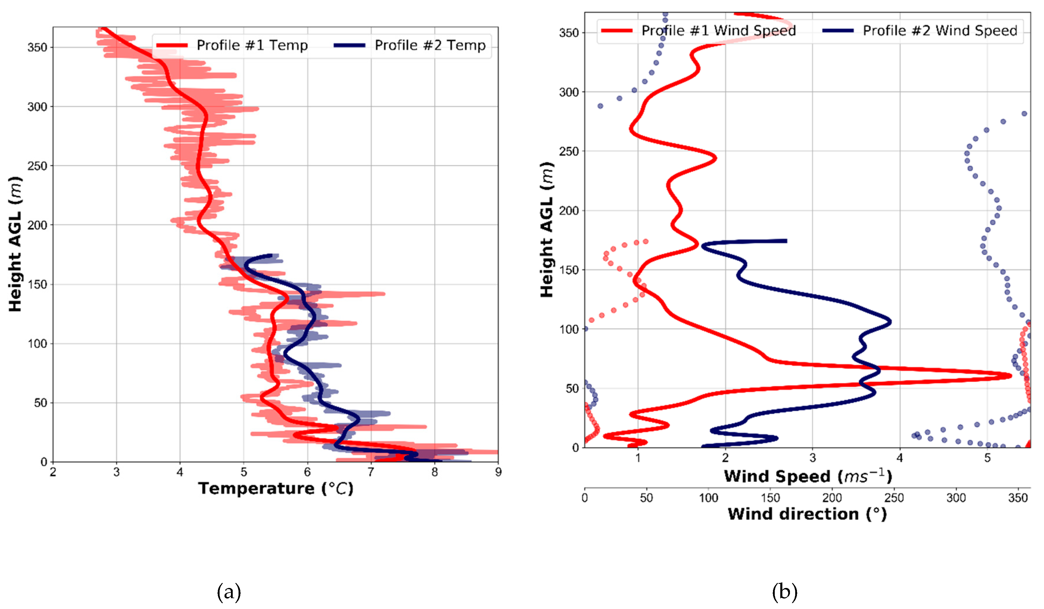
Figure 4.
(a) Low-wind time series of RMY and UAS wind speed in red and blue respectively. Bold lines represent 15 s moving average with semi-transparent representing 1 s moving average. (b) Low-wind time series of RMY and UAS sonic temperature in red and blue respectively, with time averaging noted above.
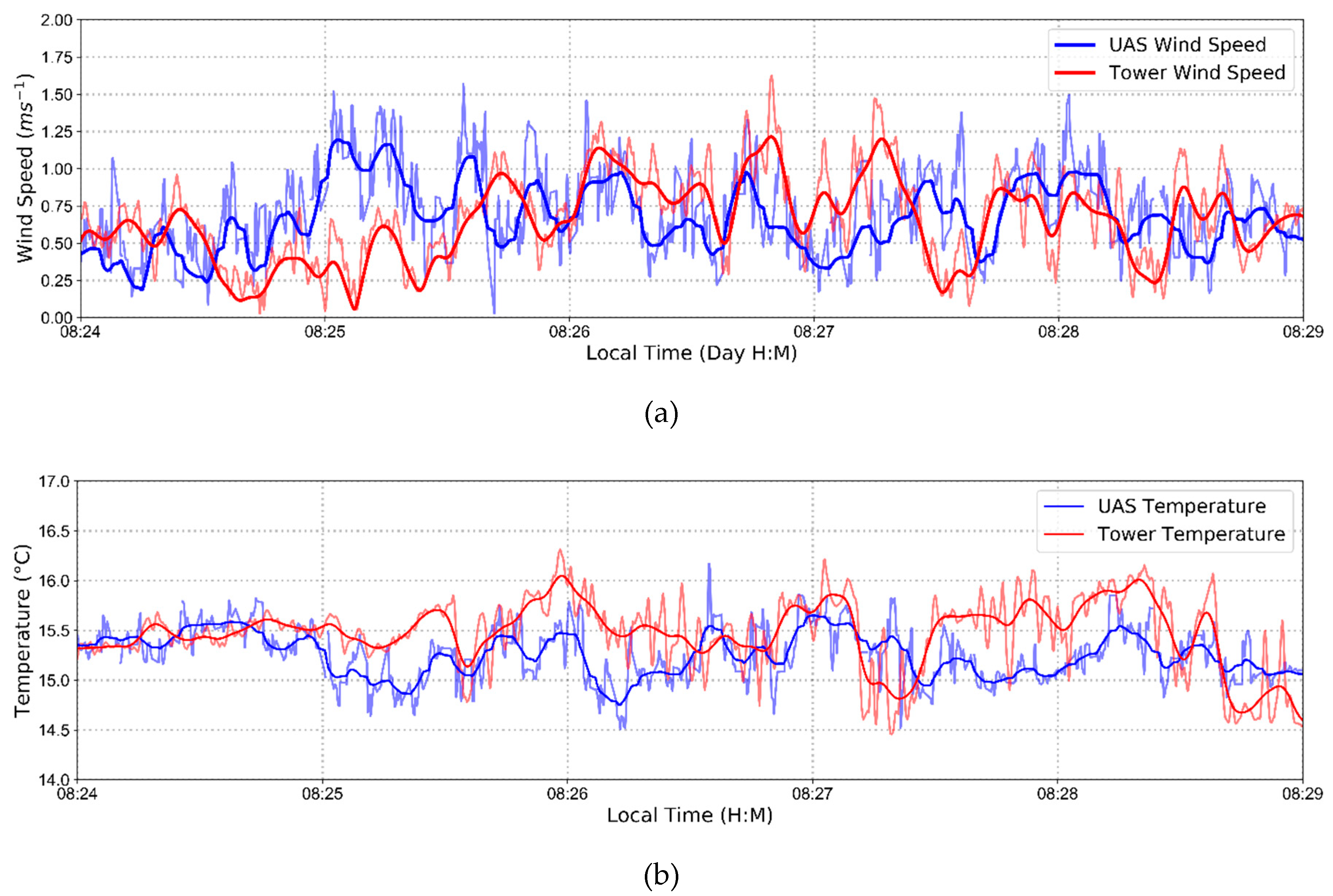
Figure 5.
(a) Flight 1 time series of RMY and UAS wind speed in red and blue, respectively. Bold lines represent 15 s moving average with semi-transparent representing 1 s moving average. (b) Flight 2 time series of RMY and UAS wind speed in red and blue respectively with time averaging noted above. (c) Scatter plot of UAS wind speed versus RMY wind speeds for both flights in blue dots. Linear regression and 95% confidence interval in blue line and shading. (d) Scatter plot of tower-mounted Trisonica wind speed versus RMY wind speeds in blue dots. Linear regression and 95% confidence interval in blue line. Note: Scales on C and D differ so as to highlight ranges of data to emphasize bias.
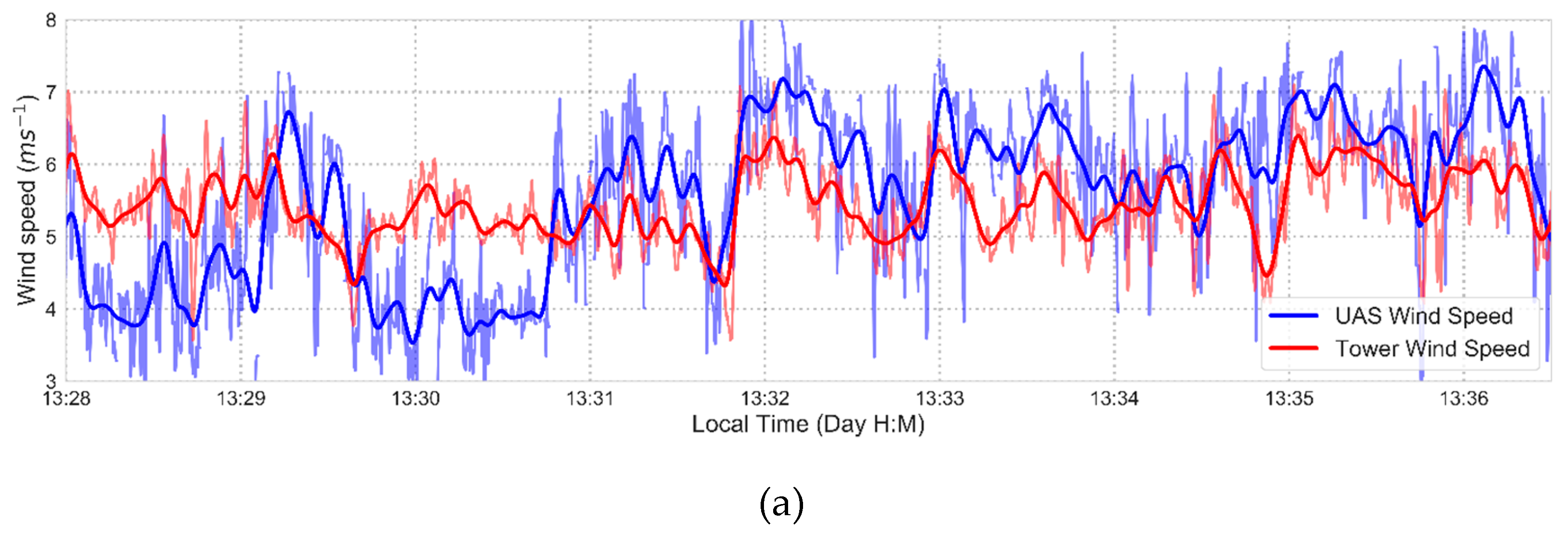

Figure 6.
(a) Flight 1 time series of RMY and UAS sonic temperature in red and blue, respectively. Bold lines represent 15 s moving average with semi-transparent representing 1 s moving average. (b) Flight 2 time series of RMY and UAS sonic temperature in red and blue respectively, with time averaging noted above. (c) Scatter plot of UAS sonic temperature versus RMY wind speeds for both flights in blue dots. Linear regression and 95% confidence interval in blue line and shading.


Table 1.
Specifications of TriSonica and RMY sonic anemometers.
| TriSonica | RMY | |
|---|---|---|
| Wind Speed | Range: 0–50 ms −1 Accuracy: (0–10 ms −1): ±0.1 ms −1 Resolution: 0.1 ms−1 | Range: 0–40 ms−1 Accuracy: (0–30 ms−1): ±1% ±0.05 ms−1 Resolution: 0.01 ms−1 |
| Wind Direction | Range: 0–360° Accuracy: ±1.0° Resolution: 1.0° | Range: 0–360° Accuracy: (0–30 ms−1): ±2° Resolution: 0.1° |
| Sonic Temperature | Range: −40 °C–80 °C Accuracy: ±2 °C Resolution: 0.1 °C | Range: −50 °C–50 °C Accuracy: (0–30 ms−1): ±2 °C Resolution: 0.01 ms−1 |
© 2020 by the authors. Licensee MDPI, Basel, Switzerland. This article is an open access article distributed under the terms and conditions of the Creative Commons Attribution (CC BY) license (http://creativecommons.org/licenses/by/4.0/).
Share and Cite
MDPI and ACS Style
Brewer, M.J.; Clements, C.B. Meteorological Profiling in the Fire Environment Using UAS. Fire 2020, 3, 36. https://doi.org/10.3390/fire3030036
AMA Style
Brewer MJ, Clements CB. Meteorological Profiling in the Fire Environment Using UAS. Fire. 2020; 3(3):36. https://doi.org/10.3390/fire3030036
Chicago/Turabian StyleBrewer, Matthew J., and Craig B. Clements. 2020. "Meteorological Profiling in the Fire Environment Using UAS" Fire 3, no. 3: 36. https://doi.org/10.3390/fire3030036