Sensitivity of the Vertical Response of Footbridges to the Frequency Variability of Crossing Pedestrians


1
Department of Construction and Manufacturing Engineering, University of Oviedo, Campus de Gijón 7.1.21, 33203 Gijón, Spain
2
Department of Construction and Manufacturing Engineering, University of Oviedo, Campus de Gijón 7.1.16, 33203 Gijón, Spain
*
Author to whom correspondence should be addressed.
†
These authors contributed equally to this work.
Vibration 2018, 1(2), 290-311; https://doi.org/10.3390/vibration1020020
Submission received: 10 October 2018
/
Revised: 22 November 2018
/
Accepted: 26 November 2018
/
Published: 30 November 2018
(This article belongs to the Special Issue Vibration Serviceability of Civil Engineering Structures)
Abstract
:Contemporary design codes and guides for vibration serviceability assessment include some simplifications in load modelling. The same statistical distribution of the inter-pedestrian variability of the step interval (frequency) is proposed for all applications. Moreover, walking loads are considered to be periodic. The intra-pedestrian variability of the step interval is neglected. A more realistic load modelling trying to overcome the limitations of the codes is intended in this paper. Instead of a single mean value of the inter-pedestrian distribution of walking speed, a range of possible variation, which account for the real variations that occur in practice depending on the footbridge location and usage, is considered. An enhanced model is proposed in this paper to reproduce statistically both the intra- and inter-pedestrian variability of the step interval as a function of the walking speed distribution. This innovative model is then applied to study the sensitivity of the vertical response of footbridges to the variability of the step interval and to evaluate the influence of the aforementioned simplifications on the predicted characteristic responses. For this purpose, low-frequency footbridges excited by single-pedestrian crossings are chosen. The response is statistically characterized through Monte Carlo numerical simulations including 720 different configurations and 10,000 load cases in each configuration. Results of the study provide an overview of the influence of the footbridge and load parameters on the responses, which can be useful in practical applications where human–structure interactions are negligible. As for the simplifications of the codes, it is found that either using a single distribution to model the inter-pedestrian variability of the spatiotemporal parameters or neglecting the intra-pedestrian variability can lead to a significant underestimation of the characteristic response of footbridges.
1. Introduction
1.1. Motivation
With the use of new materials and innovative configurations, modern structures have become more slender and prone to vibrate. This is the case of footbridges and long-span floors under pedestrian loading. As a consequence, vibration serviceability is a decisive limit state in many cases during the design stage of these kinds of structures. Due to the limitations of the contemporary codes for serviceability assessment [1], the number of structures that exhibit excessive vibration in service has grown exponentially in the last decades. This has motivated the research interest in walking-induced vibration [2]. This paper deals with the modelling of walking loads and their influence on the dynamic response of footbridges.
1.2. Considerations on Walking Modelling and Structural Response
Modelling walking loads is a complex task because they are a function of both time and space, and have a random nature. The randomness encompasses both inter- and intra-pedestrian variability. The former is related to the pedestrian-to-pedestrian variability, while the latter accounts for the variability of the same pedestrian activity at different times, as for example, the step-to-step variability of the walking load of a pedestrian in a given trial [3]. The description of the dynamic response of structures to walking loads is not straightforward because it implies many related variables. It is well known that the unimodal response of a lively structure to a single-pedestrian loading depends mainly on the average value of the step interval (frequency). The closer the step interval to the natural period (frequency) of the structure, the higher the response is. The inter-pedestrian variability of the step interval has therefore strong influence on the structural response. The response is also sensitive to the intra-pedestrian variability of the step interval. The response decreases when the variance of the step interval is increased and the average value of the step interval is close to resonance. Conversely, the response increases when the average value is out of resonance [4]. The step-to-step evolution of the deviations of the step interval with respect to the average values also affects the structural response. This means that two interval sequences having the same averages and variances but different evolutions of the deviations can lead to significant discrepancies of the structural response. This is the case, for example, when comparing the response to a pure random sequence of variations with that of an autoregressive sequence of variations with the same variance. If the evolution of the deviations of the step interval is described by an autoregressive model, the structural response is sensitive to the values of the autoregressive parameters because both the variance and the temporal evolution of the deviations of the step interval vary as a function of these parameters [5]. Considering these features, it can be established that reliable predictions of the structural response to walking loads require accurate models describing the evolution of the step interval in a trial and its inter-pedestrian variability. The value of the walking speed is also significant in the structural response. For example, two walking loads having the same temporal trace but at different walking speeds give rise to different spatial traces and, consequently, different structural responses. This is because the walking load is weighted by the modal shape in the space when integrating the structural response [6]. Thus, an accurate definition of the relationship between walking speed and step interval (or frequency) and its inter-pedestrian variability is additionally essential to obtain reliable structural responses.
1.3. State of the Art
1.3.1. Walking Load Modelling
Models of walking loads have evolved from deterministic periodic formulations to more sophisticated statistical approaches [3]. Several advanced models are available nowadays to simulate the walking loads [7,8,9]. Walking loads with statistical properties equal to that of treadmill experiments at the same walking frequency can be synthesized through these models. In [8], the step length is statistically modelled through a Gaussian distribution, which accounts for the inter-pedestrian variability. The step length, however, is assumed to be independent of the walking frequency. Under this condition, the step frequency becomes a linear function of the walking speed. Model [9] does not explicitly include the relationship between walking frequency and speed. In an application of the model to the interaction between multiple pedestrians [10], in which the walking speed is time-variant, a third-order polynomial is adopted to obtain the walking frequency as a function of the walking speed. This polynomial fits the experimental results better than the aforementioned linear function. However, the inter-pedestrian deviation of the walking frequency with respect to the polynomial trend is not taken into account. As explained in Section 1.2., these aspects have a potential influence on the dynamic response of flexible structures. Thus, these models of walking loads can be improved by refining the description of the relationships between spatiotemporal parameters and their variability. The authors of the present paper have recently developed a statistical model describing the variability of the step interval [11], for which there will be an overview in Section 2. The modelling integrates previous related findings in biomechanics and results of a campaign of treadmill tests. The individual relationship between walking frequency and speed is included in the model. It is formulated as a power law and its inter-pedestrian variability is statistically defined. However, the formulation of the autoregressive parameters of our previous model does not fit the experimental data well. Considering its influence on the structural response, an enhanced definition of the autoregressive parameters will be tried in this paper. Even though walking models are generally formulated as a function of the walking frequency in the civil engineering community, our model is formulated as a function of the walking speed. This is because when a pedestrian walks freely at a given average speed his/her nervous system controls the walking frequency (or step length) in such a manner that the metabolic energy consumption is minimized. From a mathematical point of view, it does not matter whether the walking frequency or speed are chosen as independent variable, as long as their mathematical relationship is included in the model. Moreover, the formulation on walking speed has some practical advantages. The model can be extended to real-life walking, in which the walking speed is time-variant, just by updating its parameters in each step according to the step speed. In addition, it can be applied directly to any inter-pedestrian walking speed distribution. This formulation on the basis of walking speed is very suitable to simulate individual sequences of the step intervals under dense traffic conditions. In this case, the individual walking speed is imposed by the crowd flow, which is commonly formulated as a function of the walking velocity [10,12].
1.3.2. Walking Speed
The individual walking speed distribution, which has a strong influence on the structural response, has been exhaustively studied. Whittle [13] established a typical speed of 1.40 m/s for healthy adults. Zivanovic (2012) [14] performed an experimental campaign on a steel footbridge in Podgorica, Montenegro. The pedestrian traffic was monitored with two video cameras placed at the ends of the footbridge. The average walking speed of each pedestrian was estimated dividing the footbridge length by the crossing time. She found that a normal distribution with a mean of 1.39 m/s and a standard deviation of 0.20 m/s was a close fit for the performed 2019 individual observations. Pachi and Ji [15] carried out a study of frequency and speed of people walking on two footbridges and two shopping floors placed in Manchester, UK. In each case, 100 women and 100 men were randomly selected for the test. The test subjects were not aware that they were observed so as to obtain natural results. The time elapsed for each pedestrian to cover a reference distance was measured through a stopwatch. The speed was computed from these data. They found a global average speed of 1.30 m/s in footbridges, while the average was higher in the shopping floors, with a global value of 1.40 m/s. The averages corresponding to each case were within the range of 1.23–1.43 m/s. The discrepancies with respect to the overall average speed, 1.35 m/s, were and 6%, respectively. As for the standard deviations of the individual speed, the results were within the range of 0.09–0.14 m/s, with an average value of 0.12 m/s. Kasperski and Sahnaci [16] established that for each situation in life there is a corresponding pace of life, which also influences the average walking. In this paper, a study carried out in the centre of 20 German cities is quoted. In each case, around 300 pedestrians were observed. They found that the average walking speed in each city varied within the range of 1.38–1.51 m/s. The corresponding discrepancies with respect to the overall average value, 1.45 m/s, were around . In light of these results, they recommend not to use a single value for the average walking speed when assessing the serviceability of a structure. A range of possible mean values is suggested for the walking speed instead. Chandra and Bharti [17] studied the walking speed distributions in three cities in India at different facilities. Data were collected by videographer. The analysis of results showed that the pedestrian speed was different depending on the location and facility even for the same population. The overall average speed was 1.20 m/s. Each case was within the range of 0.97–1.36 m/s. The standard deviation of an individual walking speed had an average value of 0.21 m/s and was within the range of 0.19–0.22 m/s. In all cases, the pedestrian walking speed followed the normal distribution. In our previous study [11], we measured the time elapsed by test subjects to walk a straight horizontal 35 m long path on a laboratory floor at their natural speed. From these, the corresponding walking speeds were calculated. The statistics from 150 measurements were: mean 1.41 m/s and standard deviation 0.14 m/s. Results are summarized in Table 1.
1.3.3. Sensitivity Analysis
The influence of walking variability on the vertical response of footbridges has been systematically studied by several researchers. Wan et al. [18] proposed the use of design spectra to check the vibration serviceability of footbridges under single pedestrian loading. The spectra were obtained through the probabilistic model defined in [4] considering a variety of footbridge configurations. The model included both the inter- and intra-pedestrian variability of the walking loads. The step frequency and the step length were modelled as normally distributed. However, the step length is considered to be independent from the step frequency. Moreover, the variability of the mean value of the walking frequency is not taken into account. This study proved that the peak acceleration of the response corresponding to a certain level of exceedance is more informative than the deterministic maximum acceleration recommended by the contemporary design codes and guidelines for the assessment of vibration serviceability [19,20,21,22,23,24]. Piccardo and Tubino [25] established simplified procedures to evaluate the vibration serviceability under three different traffic conditions. The procedures were aimed to avoid the computational burden required by the Monte Carlo simulations. The essential parameters governing the dynamic response were characterized through the procedures. The influence of the intra-pedestrian variability, however, is not included in the study. In a comprehensive study, Pedersen and Frier [26] investigated the sensitivity of the dynamic responses to the variability of walking parameters, which was chosen from experimental results available in the literature. Simply supported low-frequency footbridges were analysed by Monte Carlo simulations. A single value of the damping ratio is considered and the intra-pedestrian variability is not taken into account. Caprani [27] also proposed a simplified procedure to check the vibration serviceability, which accounts for both the inter- and intra-pedestrian variability. The response of an ideal footbridge was computed through the procedure and compared with that of a periodic load. The response to the load including variability was found to be significantly less than that of the periodic load. Moreover, the response was dominated by inter- rather than intra-pedestrian variability. These statements, however, cannot be generalized because they are related to a single footbridge configuration. Zivanovic et al. [28] studied the sensitivity of simulated vibration response to the randomness in frequency of jumping loads. A single-degree-of-freedom model was chosen for the simulations. Two different jumping loads were selected. One corresponded to an experimental measurement; another was generated from the measurement by preserving the measured shape and amplitude of the force but enforcing the same interval in each jump, which was set to the average achieved in the test. The response was computed for two models with different natural frequencies. One was in resonance with the second harmonic of the force, while the other was out of resonance. They found that neglecting the randomness in the jumping frequency results in overestimation of the response near resonance and underestimation away from resonance. They suggest completing the study including the sensitivity of the response to the randomness of other parameters.
1.4. Aim
The aim of this paper is twofold. A first objective is the enhancement of our previous model of step interval variability [11], focusing on the modelling of autoregressive parameters. The influence of both the intra- and inter-pedestrian variability of the step interval of human walking on the dynamic response of footbridges will be studied in a second stage through numerical simulations using the enhanced model. The human–structure interactions will not be taken into account in this study. From the sensitivity analysis, practical recommendations to check the serviceability of footbridges under single pedestrian traffic will be proposed.
2. Previous Study
The authors of the present paper carried out previously a campaign of walking tests. A statistical model describing the relationships between spatiotemporal parameters of human walking and their variability was then developed and fitted to the experimental results. Both the experimental campaign and modelling are explained in detail elsewhere [11]. An overview is presented in the next sections.
2.1. Experiments
An instrumented treadmill was used for the walking tests, in which the vertical walking forces were measured and recorded. A series of tests were carried out at six different speeds for each test subject after a warming up exercise. Subjects walked steadily around 100 m in each test. Fifty healthy adult subjects (25 men and 25 women) took part in the experiments. Information pertinent to the subjects is in Table 2. The experiments consisted of 300 tests and more than 30 km walked.
2.2. Statistical Model
In this model, the evolution of the step interval, , in a trial consists of an average value, , plus the deviations with respect to the average, ,
in which i and N denote the step number and the total steps of the trial, respectively. The deviation in a step, , is decomposed into a deterministic part due to asymmetry, , and a random part described by a second-order autoregressive process, , which is modelled as follows:
where stands for the asymmetry parameter, and represent the autoregressive parameters and is a random variable that denotes the disturbances. The average step interval for a given pedestrian, , is modelled as a power law of the walking speed, v,
in which and are the corresponding parameters. The asymmetry parameter normalized by the average step interval, , is considered constant. As for the autoregressive parameters, and , they are considered random variables independent of the walking speed, v, and which vary from trial to trial for the same pedestrian. Finally, the disturbances are considered as random variables, which vary from step to step, with normal distribution having zero mean and standard deviation, . The standard deviation is modelled as a second order polynomial of the walking speed in m/s,
in which stands for the disturbances parameter. This model reproduces the intra-pedestrian variability of the step interval in a trial as a function of the walking speed. It includes six parameters: , , , , and . The inter-pedestrian variability of these parameters is also included in the model. Parameters and are considered to be a bivariate random variable, , modelled through a binormal distribution with the following mean, , and a covariance matrix, ,
The normalized asymmetry parameter, , is modelled as a random variable having a Beta distribution with parameters: and . The autoregressive parameters, and , are considered independent random variables having a Beta distribution after the following linear transformations: , . The parameters of the corresponding Beta distributions are: , and , . This model integrates both the inter-pedestrian and the trial-to-trial variability. The disturbances parameter, , is also modelled through a Beta distribution with parameters: and .
3. Enhanced Model
The refinement of the model is focused on the autoregressive parameters, and . These parameters were estimated through Equation (2) by the least-squares method from the experimental data because the equation is linear in the parameters. Estimates of the parameters, and , for all the tests are depicted in Figure 1 as a function of walking speed.
These parameters had a certain global trend: increased with the walking speed, v, while diminished (Figure 1). In addition, there was noticeable trial-to-trial variability for each test subject. Both the trend and the variability of the identified parameters will be studied in turn in the following paragraphs. The trends of these parameters, and , have been modelled by second-order polynomials. The coefficients of the polynomials were estimated through the least-squares method, giving rise to the following values:
The fitted curves are shown in Figure 2 along with the experimental results.
The average values of the autoregressive parameters are around 0.2. These values imply that a disturbance in the interval of a given step is almost corrected in the subsequent two steps. Physically, this indicates that the step interval is controlled by the neural system in an effective manner. The outcomes also reveal that the evolution of the step interval is a weak autoregressive process. This circumstance can cause the identification of the autoregressive parameters to be inaccurate.
Let and be random variables that represent the deviations of the identified parameters, and , with respect to the experimental trends, and , for the same speed, v, that is:
The experimental realizations of these variables are shown in Figure 3. As a weak correlation was found between these variables, they are considered to be independent hereafter.
The scattering of these variables seems to be quite uniform in the range of measured speed. Consequently, it is assumed hereafter that the variances of and are speed-independent. Under this assumption, the corresponding variances and were computed from all the experimental realizations. The obtained values were: and .
A question arises at this stage: is the trial-to-trial variance of the autoregressive parameters inherent to the pedestrians or/and is it due to identification inaccuracies? To address this issue, 100 numerical simulations of the experiments were performed with the proposed model. These simulations included 30,000 trials. The values identified from the experimental data were chosen for the average step interval, , the asymmetry parameter, , and the variance of the disturbances, , while the autoregressive parameters, and , where set to their quadratic trends, and , for the same speed. Thus, the randomness inherent to the pedestrians is not included in the simulations. From these simulated series, the corresponding autoregressive parameters, and , were identified by the least-squares method. Results of one of these simulations are shown in Figure 4. As expected, the trends of the obtained parameters are very close to that of the experimental data.
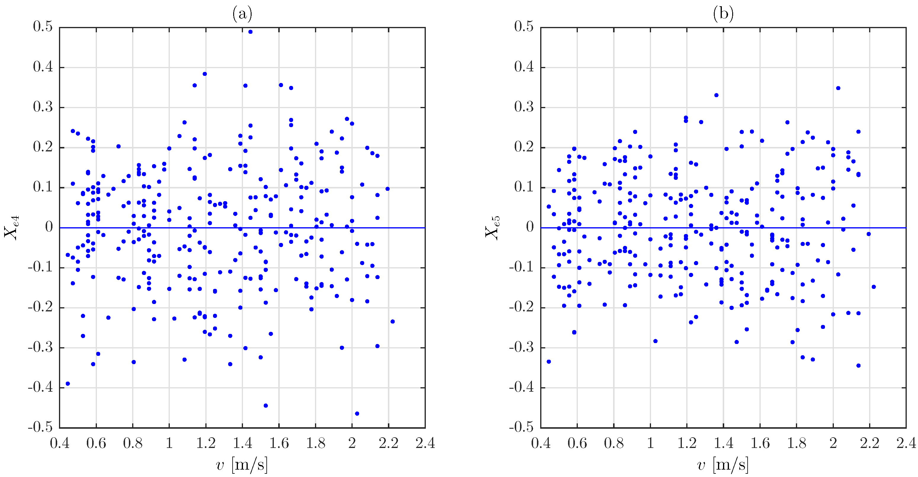
Let and be random variables that represent the deviations of the identified simulated parameters, and , with respect to the experimental trends, and , for the same speed, v, that is:
Figure 5 shows the realizations of these variables corresponding to the simulation depicted in Figure 4.
As the experimental counterpart, the scattering of the obtained deviations, and , was quite uniform and can be considered speed-independent. The variances of these deviations computed from all the simulations were: and . These variances are due exclusively to the identification inaccuracies because the variability inherent to the pedestrians was not present in the simulated data. Results indicate that the identification inaccuracies account for around 25% of the variance of the experimental deviations. The rest of the deviation, , is inherent to the pedestrians. Assuming these two causes of variability are independent, the total experimental deviations, , are equal to the identification component, , plus the inherent component, ,
Under this condition, the relationship between variances is:
From this, the values of can be calculated from the obtained values of and ,
As the realizations of the variables and are within the bounds -0.5 and 0.5 and , and can be reproduced by Beta distributions after the following linear transformation:
The variance of the Beta distribution is [29]:
where a and b are the parameters of the distribution. Results suggest a symmetric distribution. This implies equal parameters, , and the variance becomes:
From this, the parameter of the distribution of can be obtained:
Eventually, the values of the parameters of the symmetric Beta distributions of and , and , can be respectively calculated from the obtained values of (Equation (11)),
Thus, the statistical models describing the autoregressive parameters, and , are:
Statistics theory [5] establishes that the convergence of a second-order autoregressive process requires the following constrains: ; ; . Consequently, the simulations not fulfilling these constrains should be rejected in order to avoid unstable series of step intervals.
For the verification of the model, 100 numerical simulations of the experiments were carried out taking the values identified from the experimental data for the average step interval, , the asymmetry parameter, , and the variance of the disturbances, . As for the autoregressive parameters, they were calculated through the model (18) as a function of the walking speed. From the simulated series, the parameters of the model were identified. In each series of results, the identified autoregressive parameters were fitted to a quadratic polynomial and the variance of the deviations from the trend was calculated.
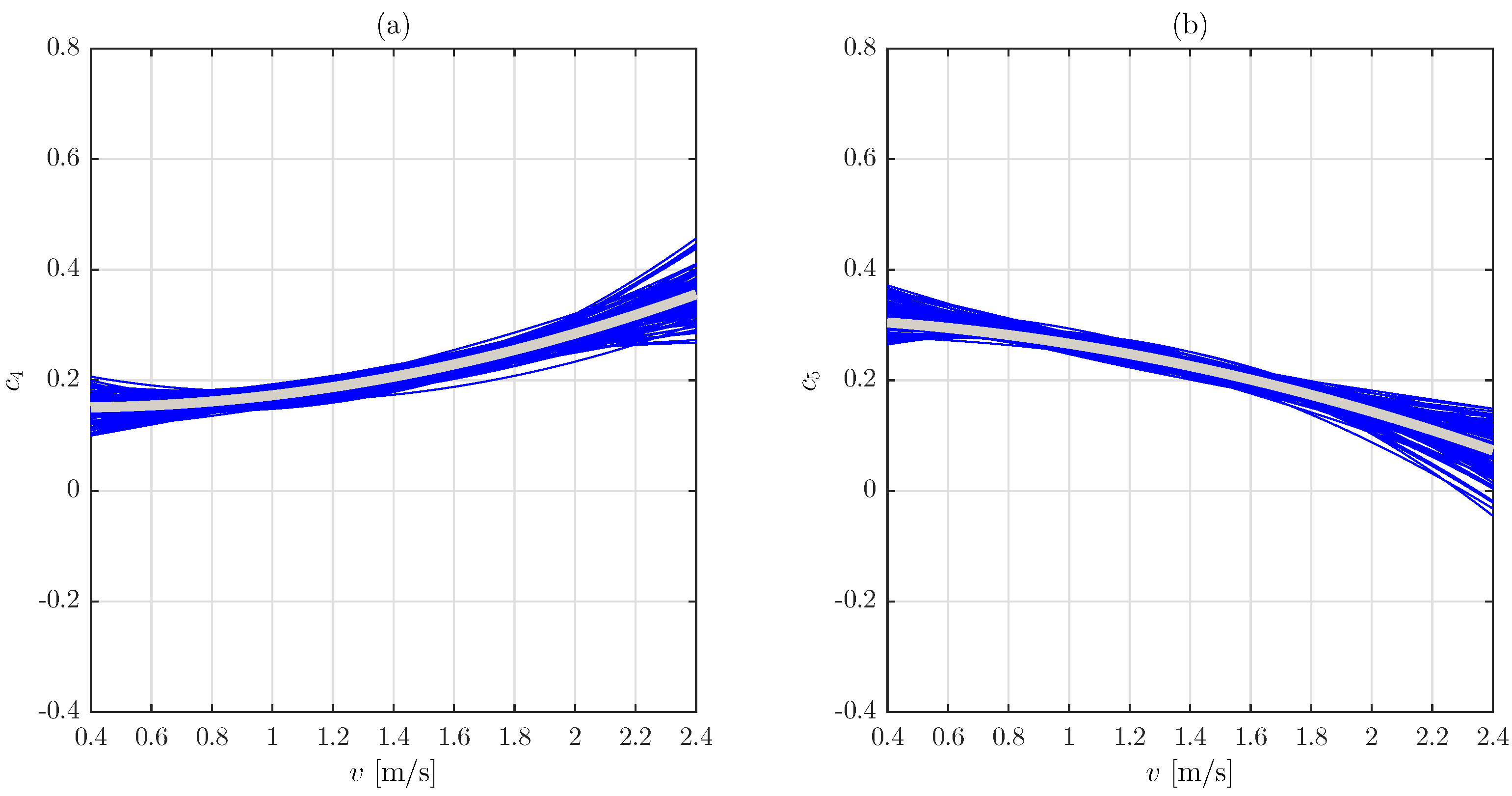
The obtained quadratic trends are depicted in Figure 6 along with the experimental trends. The simulated trends are very close and distributed around the experimental trends.
As for the variances of the deviations, their histograms are shown in Figure 7. The variances of the simulations are distributed around the experimental variances.
The values of the variances of the autoregressive parameters of our previous model are around 50% higher than those of the enhanced model (Equation (11)). Such a discrepancy has a notable effect on the corresponding structural responses.
4. Procedure for Generating Step Interval Sequences
The following scheme summarizes the procedure to generate a step interval sequence for a single pedestrian walking at constant speed under rigid soil conditions. A normal distribution with mean and standard deviation is assumed for the inter-pedestrian variability of the walking speed [14,17].
- Input data: mean, , and standard deviation, , of the walking speed and number of steps, N.
- Obtain the walking speed, v, by sampling from the distribution .
- Sample and from a binormal distribution with mean and covariance matrices of the Equation (5).
- Compute the average step interval through equation .
- Obtain the normalized asymmetry parameter, , from the Beta distribution: B(2.67, 149.10).
- Calculate the asymmetry parameter .
- Compute the autoregressive parameters, and , through Equations (18).
- If or or , go to 7; otherwise continue.
- Sample parameter from the distribution B(14.15, 561.19).
- Compute the standard deviation of disturbances, .
- Obtain the disturbances, , by sampling from a normal distribution with zero mean and standard deviation , .
- Calculate the step interval deviations and .
- Generate the step interval sequence .
5. Parametric Analysis
Simply supported beam footbridges excited by single pedestrian traffic have been chosen for this study. Different footbridge configurations and traffic conditions have been analysed. The dynamic responses have been determined through Monte Carlo numerical simulations in each case. More details of the study are presented in the following paragraphs.
5.1. Footbridge Models
Footbridges have been idealized as simply supported beams with uniform cross-section. Linear stiffness and linear viscous damping have been chosen to characterize the dynamic behaviour of the footbridges. Only the first flexural mode has been considered in the analysis. Under these conditions, the related mode had a half-sine shape. Several footbridge natural frequencies, , have been chosen for the study, namely from 1.4 Hz to 2.8 Hz every 0.1 Hz. These are within the common range of excitation of the first harmonic of the walking loads. Different footbridge lengths have been selected for the analysis: L=12.5, 25, 50 and 100 m. As the liveliness of a footbridge is mainly governed by the magnitude of damping, the following low values of the modal damping ratio have been chosen: 0.25, 0.5, 1 and 2%.
5.2. Walking Loads
The individual walking load has been modelled as a single variable force moving along the footbridge at constant speed. Only the fundamental Fourier harmonic of the walking load is considered in each step. The amplitude of this harmonic, F, was assumed to be the same for all the steps of a trial. Thus, the influence of the step interval variability on the response of footbridges is isolated. Two different models have been adopted for the temporal evolution of the step interval. They will be referred to as quasiperiodic model and periodic model hereafter. The step interval is considered to be variable in the quasiperiodic model. The corresponding sequence of step intervals was computed through the procedure outlined in Section 4 as a function of the walking speed. The step interval is considered to be constant in the periodic model. It was set to the average step interval, . Its value was computed as a function of the walking speed through the first four items of the procedure in Section 4. The quasiperiodic model, therefore, integrates both the inter- and intra-pedestrian variability, while the periodic model only includes the inter-pedestrian variability.
5.3. Walking Speed
The statistical properties of the distribution of the individual walking speeds were estimated from the literature review in Section 1.3.1. The following working hypotheses were established. The individual walking speed of a given population is statistically described by a normal distribution. Even for the same population, the parameters of the walking speed distribution depend on the type of structure considered and its geographic location. A range of variation is considered for the mean of the distribution instead of a single value. In this study, a normal distribution is considered for the individual walking speed, with a mean of 1.40 m/s and standard deviation of 0.14 m/s. These parameters are consistent with our experimental results. Additional values at of the reference mean, 1.4 m/s, which are consistent with the outcomes of the revised literature, were also considered. Thus, the following series of means: 1.26, 1.40 and 1.54 m/s was additionally used in the simulations. These two approaches of the speed distributions will be referred to as single mean and multiple means hereafter.
5.4. Walking Frequency
The distribution of walking frequency is obtained from that of walking speed in this section. Our model includes the deterministic relationship between both the walking speed and the step interval for a given pedestrian (Equation (3)) and the inter-pedestrian stochastic variability of its parameters (Equation (5)). Therefore, the distribution of the walking frequency can be determined from that of the walking speed through the model. The distributions of the walking frequency corresponding to the three considered distributions of walking speed were achieved from Monte Carlo numerical simulations. For this purpose, 100,000 values of the average step interval, , were computed through the first four items of the procedure in Section 4 for each distribution of walking speed. The corresponding average walking frequencies, , were calculated from them, . The statistical analysis proved that a log-normal distribution fit the results better than a normal distribution, as is shown in Figure 8. The mean and standard deviation of the walking frequency, and , were estimated from the results by the maximum likelihood method considering a log-normal distribution. Outcomes are shown in Table 3 alongside those of the corresponding walking speed. The statistics of the obtained distribution are close to those identified directly from measurements on people walking freely on footbridges and shopping centers in other European countries [14,15]. The walking frequency corresponding to the reference walking speed mean, 1.4 m/s, is 2.05 Hz. The considered increments for the reference walking speed mean, m/s, give rise to frequency increments of Hz.
5.5. Computation and Characterization of Responses
The individual footbridge responses were computed in the modal space considering the footbridge as a single-degree-of-freedom dynamic system. The procedure did not account for potential changes in mass, damping and stiffness of human–structure interactions and consisted of the following stages. The analytical spatial load was numerically sampled at regular intervals, 0.001 s. The load was transformed to the modal space by weighting the spatial load by the modal shape. The discrete load was converted to the frequency domain through the fast Fourier transform. The dynamic response was then evaluated in the frequency domain multiplying the force by the frequency response function of the dynamic system. The displacement response in the time domain was obtained via the inverse fast Fourier transform. Eventually, the modal acceleration response was evaluated from the displacements through the second central difference method. The response was characterized by the peak acceleration, , in each trial. was defined as the maximum absolute modal acceleration of the footbridge.
A vertical harmonic load applied at the midspan of the footbridge is considered now, its amplitude being equal to that of the fundamental Fourier harmonic of the walking load, F. Taking into account the low value of the damping ratio adopted in this study, the maximum amplitude of the steady-state acceleration response to this virtual load can be approximated by that corresponding to resonance [30].
in which m and stand for the modal mass and damping ratio of the footbridge, respectively. The steady-state acceleration constitutes an upper limit of the peak acceleration caused by the corresponding walking load. This is so because the steady-state acceleration is theoretically reached after an infinite number of cycles of the virtual load, while the walking load has a limited number of cycles (steps), which depend on the footbridge length and walking speed. Moreover, the amplitude of the virtual load has the same value in all the cycles, while the amplitude of the walking load is modulated by the local mode shape amplitude which is less than or equal to 1. Eventually, the peak acceleration was normalized to the steady-state acceleration,
Thus, the normalized response, , is a dimensionless variable bounded in the interval 0–1. Another interesting property of the normalized response is its independence of both the force amplitude, F, and the modal mass, m. Indeed, for the considered walking load the peak acceleration is proportional to the amplitude, F, and inversely proportional to the modal mass, m, according to the Duhamel integral [30],
Consequently, when dividing Equation (21) by Equation (19) to obtain the normalized response (Equation (20)) both F and m are cancelled. This normalization causes the dimensionality of the case to be reduced and allows the outcomes to be presented in a more compact manner.
10,000 random simulations were carried out for each footbridge and load configuration. The number of simulations was set after some trials and constituted a trade-off between time of computation and statistical accuracy of the results. The corresponding 10,000 normalized responses were sorted in ascending order. Eventually, the 9500:10,000 order statistic was chosen as an estimation of the 95 percentile of the distribution of the given configuration, . This statistic was used to characterize the response of the considered footbridge configurations and loads. It will be referred to as characteristic normalized response hereafter.
5.6. Campaign of Simulations
Three different cases labelled as A, B and C were considered in this study. Approach A was the most complete including the variability of both the mean speed and the step interval. Approaches B and C were simplifications of approach A, in which the variability of the mean speed and the step interval, respectively, were not considered. The particularities of these approaches are summarized in Table 4. This arrangement allowed the influence of the variability of different parameters on the footbridge responses to be studied just by comparing the outcomes. The campaign included 720 different configurations and 7,200,000 single pedestrian crossing simulations.
5.7. Results and Discussion
5.7.1. Approach A
The spectra of the characteristic normalized response were obtained as the envelope of those corresponding to the three mean speeds considered, 1.26, 1.40 and 1.54 m/s. They are depicted in Figure 9. Spectra have a bell-like shape in all the considered configurations, which exhibit a shoulder on the top. The limits of the shoulders vary approximately from 1.7–2.5 Hz for m to 1.8–2.3 Hz for m. These ranges correspond to the central part of the considered walking frequency distributions (Table 3). The limits have a value approximately equal to . Spectra are almost constant in this part. Outside this central part, i.e., in the tails of the frequency distributions, the characteristic response tends progressively to zero.
The maxima of the spectra, , are placed within the frequency interval 2.0–2.1 Hz. This frequency interval is consistent with the walking frequency distributions derived from the adopted walking speed distributions in Section 5.4. These distributions have the maximum probability density within this interval (Figure 8 and Table 3). The maxima are shown in Figure 10 as a function of the footbridge length and damping ratio. Their trend is clear. The maxima increase when the footbridge length or the damping ratio is increased. This means that the higher the footbridge length or the damping ratio, the closer the maximum characteristic acceleration is to the steady acceleration. The justification for these results is that the characteristic response corresponds to walking loads close to resonance. Under this condition, the amplitude of the acceleration response approaches asymptotically to that of the steady response when the number of excitation cycles (steps) is increased [30]. As the number of steps of a crossing is proportional to the footbridge length, the characteristic response approaches asymptotically to 1 as a function of the footbridge length. The number of cycles (steps) to reach a proportion of the amplitude of the steady response is inversely proportional to the damping ratio [30]. Therefore, the lower the damping ratio, the higher the number of steps (footbridge length) to reach the same characteristic response.
5.7.2. Approach B
Figure 11 shows the response spectra of approach B. The response spectra of approach A are superimposed for comparison. Spectra B are sharper than spectra A as a consequence of the use of a single-mean speed. The values of the maxima of spectra B, however, are very close to those of spectra A. In order to compare qualitatively both approaches, the spectra B were divided by the spectra A. The corresponding ratios are shown in Figure 12. Spectra B are very close to spectra A within a central range of frequencies. The width of this range diminishes progressively as a function of the footbridge length. The bounds of the range vary from 1.8–2.4 Hz for m to 2.0–2.1 Hz for m. Spectra B are always lower than spectra A outside these ranges, i.e., approach B underestimates the characteristic response.
The maximum discrepancy between spectra B and A is almost independent of the footbridge length and increases when the damping ratio is diminished (Figure 13). Results range from 51% for to 68% for .
5.7.3. Approach C
Spectra of approach C are depicted in Figure 14 along with those of approach A. Spectra C are also sharper than spectra A because the intra-pedestrian variability is not included in this approach. Figure 15 shows the ratio of spectra C to the spectra A. Spectra C are also close to spectra A within a central range of frequencies. The width of this range diminishes progressively as a function of the footbridge length. The bounds of the range vary from 1.6–2.6 Hz for m to 1.9–2.2 Hz for 0 m. Within these ranges, spectra C are slightly higher than spectra A in almost all cases. Thus, approach C slightly overestimates the characteristic response. Outside these ranges, however, approach C always underestimates the characteristic response. The maximum discrepancy between spectra C and A within the analysed range of footbridge frequencies, 1.4–2.8 Hz, is very low and almost independent of the damping ratio for m (Figure 16). This discrepancy increases when either the footbridge length is increased or the damping ratio is diminished. For m, the maximum discrepancy ranges from 33% for to 56% for .
5.8. Practical Procedure for Vibration Serviceability Checking
The outcomes of the parametric study are advantageously used to assess the vibration serviceability of footbridges. A practical procedure is proposed to obtain the characteristic vertical response of footbridges to single pedestrian crossings. The procedure is based on the response spectra of approach A, which include both the intra-pedestrian variability of the walking frequency and the variability of the mean walking speed (frequency). It follows from Figure 11 that spectra A can be obtained approximately by moving horizontally to the right and left the corresponding spectra B, the magnitude of the displacement being equal to the expected variations of the mean frequency obtained in Section 5.4, Hz. The cost to compute spectra A is drastically reduced with this approximated procedure.
A given case is defined by the footbridge frequency, , length, L, damping ratio, , modal mass, m, and amplitude of the fundamental harmonic of the walking load, F. The corresponding normalized response, (, L, ), is obtained from the spectra of approach A as a function of , L, . The normalized response is estimated from the curves on Figure 9 by linear interpolation. According to Equations (19) and (20), the characteristic peak acceleration is finally obtained by multiplying the characteristic normalized response by the related steady-state acceleration, (, m, F), i.e.,
6. Conclusions
A statistical model describing the relationships between spatiotemporal parameters of human walking and their variability, which was previously developed by the authors, has been enhanced in this paper. A refinement is introduced to the autoregressive parameters of the model. These parameters are decomposed into deterministic and random parts. The deterministic component is described by a second-order polynomial of the walking speed. The random component varies from trial to trial even for the same pedestrian. It is modelled through a symmetric Beta distribution.
The vertical response of low-frequency simply supported footbridges to single pedestrian crossing has been studied through Monte Carlo simulations based on the enhanced model. The simulations included different footbridge and load configurations. Results have been condensed into dimensionless characteristic response spectra. The study has been very instructive and allows several conclusions to be drawn. Overall, it can be concluded that the vertical dynamic response of low-frequency footbridges to single-pedestrian crossings is very sensitive to both the intra- and inter-pedestrian variability of the walking frequency. It is found in the studied cases that using a single statistical distribution for the inter-pedestrian walking speed (frequency) leads to inaccuracies up to 68% in the predictions of the characteristic response. The inaccuracies are up to 56% when the intra-pedestrian variability of the step interval (frequency) is neglected.
Specifically, the use of an interval of variation for the mean of the inter-pedestrian distribution of the walking speed (frequency) is more suitable than a single value. This interval accounts for the variations that occur in practice depending on the use of the footbridge and its geographic location even for the same population. The limits of these intervals can be estimated as of the mean speed of the reference population. An expeditious procedure is proposed to obtain the spectra corresponding to variable mean speed from those of single mean speed. When considering this interval, the spectra show a flat shape within the central part of the inter-pedestrian distribution or walking frequency. The limits of this central part can be estimated as the mean plus and minus the standard deviation of the walking frequency of the reference population. The response of footbridges can be estimated through periodic walking loads within this central interval. Outside the interval, however, the periodic model can significantly underestimate the response. More sophisticated models including the intra-pedestrian variability of the step interval should be considered in this case. Based on the results, a procedure is suggested to obtain the characteristic response of footbridges under single pedestrian loading. The procedure could be used for designing footbridges under low-density pedestrian traffic, where the single pedestrian loading is the most probable scenario and the human–structure interaction is negligible. The model, however, should be completed including more harmonics and subharmonics of the walking force and their variability.
Author Contributions
Each author contributes equally in both research and writing of this manuscript.
Funding
This research received no external funding.
Conflicts of Interest
The authors declare no conflict of interest.
References
- Živanović, S.; Pavic, A.; Ingólfsson, E.T. Modeling Spatially Unrestricted Pedestrian Traffic on Footbridges. J. Struct. Eng. 2010, 136, 1296–1308. [Google Scholar] [CrossRef] [Green Version]
- Živanović, S.; Pavic, A.; Reynolds, P. Vibration serviceability of footbridges under human-induced excitation: A literature review. J. Sound Vib. 2005, 279, 1–74. [Google Scholar] [CrossRef] [Green Version]
- Racic, V.; Brownjohn, J.M.W. Experimental identification and analytical modelling of human walking forces: Literature review. J. Sound Vib. 2009, 326, 1–49. [Google Scholar] [CrossRef]
- Živanović, S.; Pavic, A. Quantification of Dynamic Excitation Potential of Pedestrian Population Crossing Footbridges. Shock Vib. 2011, 18, 563–577. [Google Scholar] [CrossRef]
- Yaffee, R.A.; McGee, M. Introduction to Time Series Analysis and Forecasting: With Applications of SAS and SPSS; Academic Press, Inc.: New York, NY, USA, 2000. [Google Scholar]
- Bocian, M.; Brownjohn, J.M.W.; Racic, V.; Hester, D.; Quattrone, A.; Monnickendam, R. A framework for experimental determination of localised vertical pedestrian forces on full-scale structures using wireless attitude and heading reference systems. J. Sound Vib. 2016, 376, 217–243. [Google Scholar] [CrossRef] [Green Version]
- Brownjohn, J.M.W.; Pavic, A.; Omenzetter, P. A spectral density approach for modelling continuous vertical forces on pedestrian structures due to walking. Can. J. Civ. Eng. 2004, 31, 65–77. [Google Scholar] [CrossRef] [Green Version]
- Živanović, S.; Pavic, A.; Reynolds, P. Probability-based prediction of multi-mode vibration response to walking excitation. Eng. Struct. 2007, 29, 942–954. [Google Scholar] [CrossRef]
- Racic, V.; Brownjohn, J.M.W. Stochastic model of near-periodic vertical loads due to humans walking. Adv. Eng. Inform. 2011, 25, 259–275. [Google Scholar] [CrossRef]
- Venuti, F.; Racic, V.; Corbetta, A. Modelling framework for dynamic interaction between multiple pedestrians and vertical vibrations of footbridges. J. Sound Vib. 2016, 379, 245–263. [Google Scholar] [CrossRef]
- García-Diéguez, M.; Zapico-Valle, J.L. Statistical Modeling of the Relationships between Spatiotemporal Parameters of Human Walking and Their Variability. J. Struct. Eng. 2017, 143, 04017164. [Google Scholar] [CrossRef]
- Venuti, F.; Bruno, L. Crowd-structure interaction in lively footbridges under synchronous lateral excitation: A literature review. Phys. Life Rev. 2009, 6, 176–206. [Google Scholar] [CrossRef] [PubMed]
- Whittle, M. Gait Analysis: An Introduction; Butterworth-Heinemann Elsevier: Oxford, UK, 2007. [Google Scholar]
- Živanović, S. Benchmark Footbridge for Vibration Serviceability Assessment under the Vertical Component of Pedestrian Load. J. Struct. Eng. 2012, 138, 1193–1202. [Google Scholar] [CrossRef] [Green Version]
- Pachi, A.; Ji, T. Frequency and velocity of people walking. Struct. Eng. 2005, 83, 36–40. [Google Scholar]
- Sahnaci, C.; Kasperski, M. Random loads induced by walking. Proc. Eurodyn 2005, 1, 441–446. [Google Scholar]
- Chandra, S.; Bharti, A.K. Speed Distribution Curves for Pedestrians during Walking and Crossing. Procedia Soc. Behav. Sci. 2013, 104, 660–667. [Google Scholar] [CrossRef]
- Wan, K.; Živanović, S.; Pavic, A. Design Spectra for Single Person Loading Scenario on Footbridges. In Proceedings of the IMAC-XXVII, Orlando, FL, USA, 9–12 February 2009. [Google Scholar]
- International Organization for Standardization. ISO 10137: Bases for Design of Structures-Serviceability of Buildings and Pedestrian Structures against Vibration; ISO: Geneva, Switzerland, 2007. [Google Scholar]
- Association Francaise de Génie Civil; Sétra/AFGC. Assesment of Vibrational Behaviour of Footbridges under Pedestrian Loading; SETRA: Paris, France, 2006. [Google Scholar]
- Human Induced Vibration of Steel Structures. Design of Footbridges, Guidelines. 2008. Available online: http://www.stb.rwth-aachen.de/projekte/2007/HIVOSS/download.php (accessed on 29 November 2018).
- BSI. Steel, Concrete and Composite Bridges. Specification for Loads, BS 5400: Part 2; British Standard Institution: London, UK, 1978. [Google Scholar]
- UK National Annex to Eurocode 1: Actions on Structures—Part 2: Traffic Loads on Bridges; NA to BS EN 1991–2:2003; British Standards Institution: London, UK, 2008.
- Eurocode 5: Design of Timber Structures—Part 2: Bridges; EN 1995–2:2004; British Standards Institution: London, UK, 2004.
- Piccardo, G.; Tubino, F. Simplified procedures for vibration serviceability analysis of footbridges subjected to realistic walking loads. Comput. Struct. 2009, 87, 890–903. [Google Scholar] [CrossRef]
- Pedersen, L.; Frier, C. Sensitivity of footbridge vibrations to stochastic walking parameters. J. Sound Vib. 2010, 329, 2683–2701. [Google Scholar] [CrossRef]
- Caprani, C.C. Application of the pseudo-excitation method to assessment of walking variability on footbridge vibration. Comput. Struct. 2014, 132, 43–54. [Google Scholar] [CrossRef]
- McDonald, M.G.; Živanović, S. Measuring Ground Reaction Force and Quantifying Variability in Jumping and Bobbing Actions. J. Struct. Eng. 2017, 143, 04016161. [Google Scholar] [CrossRef]
- Rohatgi, V.K.; Ehsanes Saleh, A.K.M. An Introduction to Probability and Statistics; John Wiley & Sons: Hoboken, NJ, USA, 2011. [Google Scholar]
- Clough, R.W.; Penzien, J. Dynamics of Structures, 2nd ed.; McGraw-Hill: New York, NY, USA, 1993. [Google Scholar]
Figure 1.
Autoregressive parameters vs walking speed. Experimental results for all the test subjects. (a) Parameter ; (b) parameter .
Figure 1.
Autoregressive parameters vs walking speed. Experimental results for all the test subjects. (a) Parameter ; (b) parameter .

Figure 2.
Autoregressive parameters identified from the experimental data vs walking speed. Dots: experimental results. Line: quadratic trend. (a) parameter ; (b) parameter .
Figure 2.
Autoregressive parameters identified from the experimental data vs walking speed. Dots: experimental results. Line: quadratic trend. (a) parameter ; (b) parameter .

Figure 3.
Deviations of the experimental parameters and with respect to their quadratic trends, and , vs walking speed. (a) ; (b) .
Figure 3.
Deviations of the experimental parameters and with respect to their quadratic trends, and , vs walking speed. (a) ; (b) .

Figure 4.
Autoregressive parameters identified from the simulated data vs walking speed. Dots: results from simulated data. Lines: quadratic trend. Discontinuous: Experiments. Continuous: Simulations. (a) ; (b) .
Figure 4.
Autoregressive parameters identified from the simulated data vs walking speed. Dots: results from simulated data. Lines: quadratic trend. Discontinuous: Experiments. Continuous: Simulations. (a) ; (b) .

Figure 5.
Deviations of the simulated parameters and with respect to the experimental quadratic trends, and , vs walking speed. (a) ; (b) .
Figure 5.
Deviations of the simulated parameters and with respect to the experimental quadratic trends, and , vs walking speed. (a) ; (b) .

Figure 6.
Quadratic trends of the autoregressive parameters vs walking speed. Grey bold line: experiments. Fine lines: simulations. (a) ; (b) .
Figure 6.
Quadratic trends of the autoregressive parameters vs walking speed. Grey bold line: experiments. Fine lines: simulations. (a) ; (b) .

Figure 7.
Histogram of the variances of the simulations. Line: experimental value. (a) ; (b) .
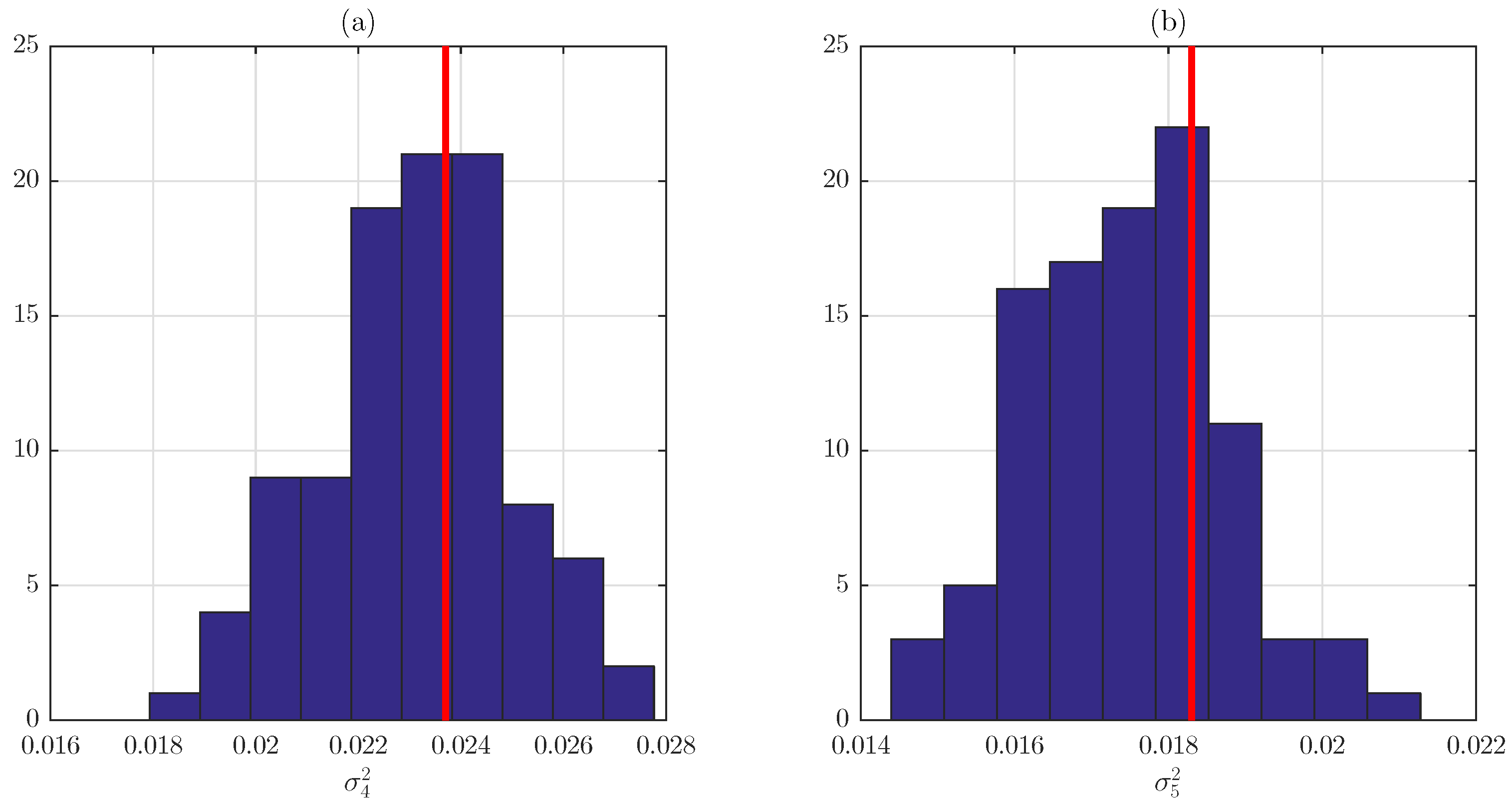
Figure 8.
Probability density function of the walking frequency corresponding to a mean walking speed of 1.4 m/s. Bold line: Normal fit. Fine line: Log-normal fit. Bars: Simulations.
Figure 8.
Probability density function of the walking frequency corresponding to a mean walking speed of 1.4 m/s. Bold line: Normal fit. Fine line: Log-normal fit. Bars: Simulations.
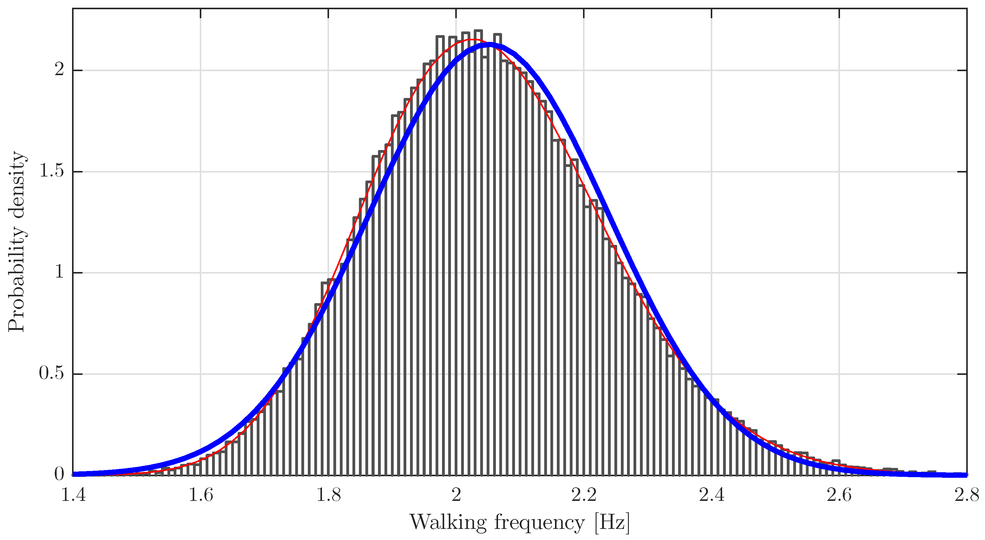
Figure 9.
Response spectra of approach A. (a): m, (b): m, (c): m, (d): m. Marks: *: , ∘: , +: and □: .
Figure 9.
Response spectra of approach A. (a): m, (b): m, (c): m, (d): m. Marks: *: , ∘: , +: and □: .

Figure 10.
Maxima of the response spectra of approach A versus footbridge length, L. Marks: *: , ∘: , +: and □: .
Figure 10.
Maxima of the response spectra of approach A versus footbridge length, L. Marks: *: , ∘: , +: and □: .

Figure 11.
Response spectra. Bold lines: approach B. Fine lines: approach A. (a): m, (b): m, (c): m, (d): m. Marks: *: , ∘: , +: and □: .
Figure 11.
Response spectra. Bold lines: approach B. Fine lines: approach A. (a): m, (b): m, (c): m, (d): m. Marks: *: , ∘: , +: and □: .

Figure 12.
Ratio of the spectra B to the spectra A. (a): m, (b): m, (c): m, (d): m. Marks: *: , ∘: , +: and □: .
Figure 12.
Ratio of the spectra B to the spectra A. (a): m, (b): m, (c): m, (d): m. Marks: *: , ∘: , +: and □: .
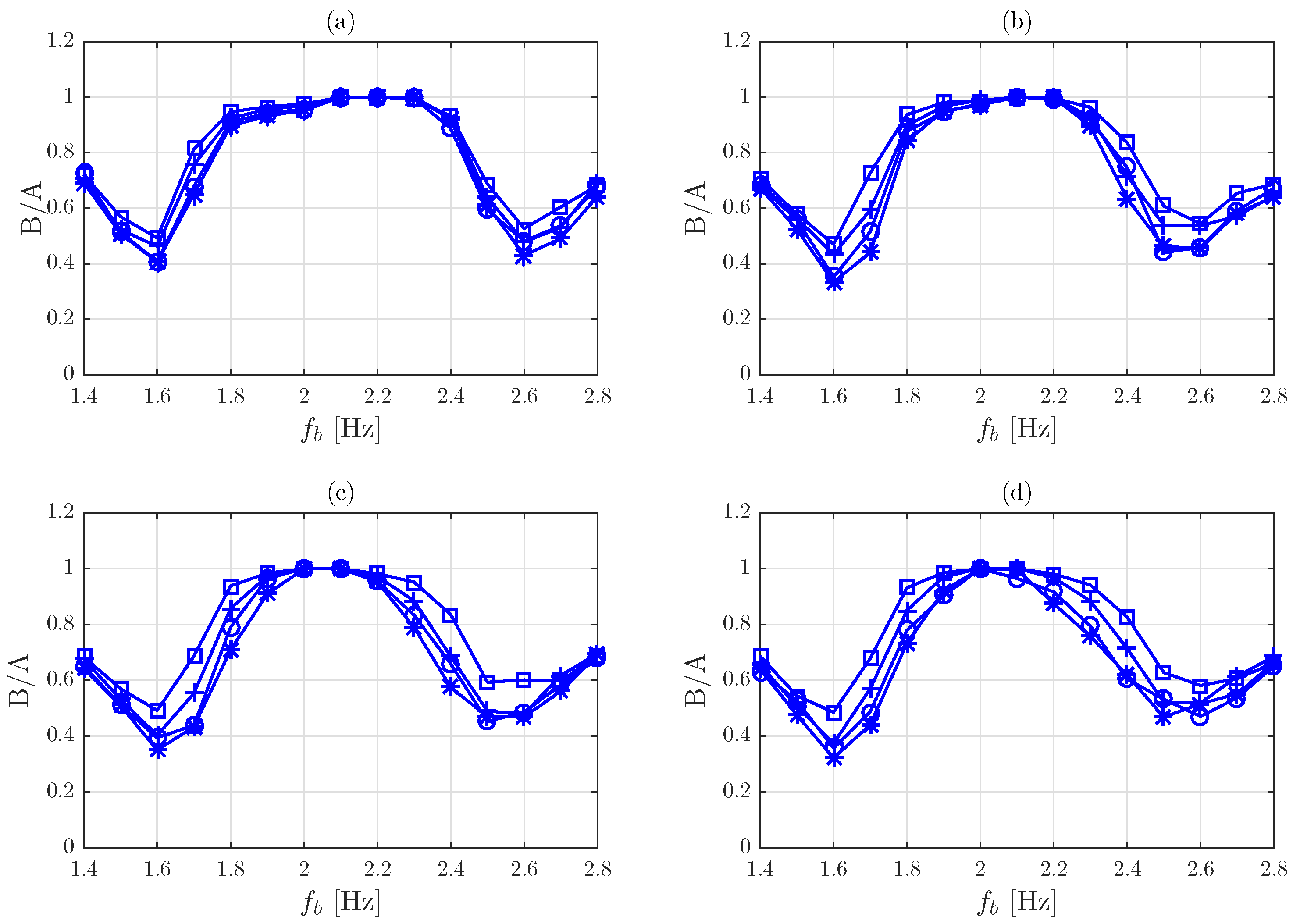
Figure 13.
Maximum discrepancy between spectra B and A versus footbridge length, L. Marks: *: , ∘: , +: and □: .
Figure 13.
Maximum discrepancy between spectra B and A versus footbridge length, L. Marks: *: , ∘: , +: and □: .

Figure 14.
Response spectra. (a): m, (b): m, (c): m, (d): m. Bold lines: approach C. Fine lines: approach A. Marks: *: , ∘: , +: and □: .
Figure 14.
Response spectra. (a): m, (b): m, (c): m, (d): m. Bold lines: approach C. Fine lines: approach A. Marks: *: , ∘: , +: and □: .

Figure 15.
Ratio of the spectra C to the spectra A. (a): m, (b): m, (c): m, (d): m. Marks: *: , ∘: , +: and □: .
Figure 15.
Ratio of the spectra C to the spectra A. (a): m, (b): m, (c): m, (d): m. Marks: *: , ∘: , +: and □: .

Figure 16.
Maximum discrepancy between spectra C and A versus footbridge length, L. Marks: *: , ∘: , +: and □: .
Figure 16.
Maximum discrepancy between spectra C and A versus footbridge length, L. Marks: *: , ∘: , +: and □: .


Table 1.
Statistics of walking speed.
| Reference | Mean (m/s) | Standard Deviation (m/s) | Country | No Samples |
|---|---|---|---|---|
| Whittle [13] | 1.40 | - | - | - |
| Zivanovic [14] | 1.39 | 0.20 | Montenegro | 2019 |
| Pachi and Ji [15] | 1.23–1.43 | 0.09–0.14 | UK | 200 |
| Kasperski and Sahnaci [16] | 1.38–1.51 | - | Germany | 6000 |
| Chandra and Bharti [17] | 0.97–1.36 | 0.19–0.22 | India | 1523 |
| García-Diéguez and Zapico-Valle [11] | 1.41 | 0.14 | Spain | 150 |
Table 2.
Information about the test subjects.
| Unit | Mean | Standard Deviation | Minimum | Maximum | |
|---|---|---|---|---|---|
| Age | year | 41.2 | 11.8 | 22.0 | 71.0 |
| Mass | kg | 74.4 | 15.3 | 41.5 | 125.6 |
| Height | m | 1.72 | 0.09 | 1.54 | 1.93 |
Table 3.
Mean and standard deviation of the walking frequency, and , related to those of the walking speed, and .
Table 3.
Mean and standard deviation of the walking frequency, and , related to those of the walking speed, and .
| (Hz) | (Hz) | (m/s) | (m/s) |
|---|---|---|---|
| 1.94 | 0.19 | 1.26 | 0.14 |
| 2.05 | 0.19 | 1.40 | 0.14 |
| 2.16 | 0.19 | 1.54 | 0.14 |
Table 4.
Approaches considered in the simulations.
| Approach | Load Model | Distributions of Walking Speed |
|---|---|---|
| A | Quasiperiodic | Multiple mean (1.26, 1.40 and 1.54 m/s) |
| B | Quasiperiodic | Single mean (1.40 m/s) |
| C | Periodic | Multiple mean (1.26, 1.40 and 1.54 m/s) |
© 2018 by the authors. Licensee MDPI, Basel, Switzerland. This article is an open access article distributed under the terms and conditions of the Creative Commons Attribution (CC BY) license (http://creativecommons.org/licenses/by/4.0/).
Share and Cite
MDPI and ACS Style
García-Diéguez, M.; Zapico-Valle, J.L. Sensitivity of the Vertical Response of Footbridges to the Frequency Variability of Crossing Pedestrians. Vibration 2018, 1, 290-311. https://doi.org/10.3390/vibration1020020
AMA Style
García-Diéguez M, Zapico-Valle JL. Sensitivity of the Vertical Response of Footbridges to the Frequency Variability of Crossing Pedestrians. Vibration. 2018; 1(2):290-311. https://doi.org/10.3390/vibration1020020
Chicago/Turabian StyleGarcía-Diéguez, Marta, and Jose Luis Zapico-Valle. 2018. "Sensitivity of the Vertical Response of Footbridges to the Frequency Variability of Crossing Pedestrians" Vibration 1, no. 2: 290-311. https://doi.org/10.3390/vibration1020020