
A Testbench for Measuring the Dynamic Force-Displacement Characteristics of Shockmounts

1
Department of Mechanical Engineering, Helmut Schmidt University, Holstenhofweg 85, 22043 Hamburg, Germany
2
Bundeswehr Technical Center for Ships and Naval Weapons, Maritime Technology and Research, Berliner Straße 115, 24340 Eckernförde, Germany
*
Author to whom correspondence should be addressed.
Vibration 2024, 7(1), 1-35; https://doi.org/10.3390/vibration7010001
Submission received: 11 August 2023
/
Revised: 9 November 2023
/
Accepted: 30 November 2023
/
Published: 21 December 2023
Abstract
:Shockmounts in naval applications are used to mount technical equipment onto the structure of naval vessels. The insulating effect against mechanical shock is important here, as it can excite the structure in the event of underwater explosions and otherwise cause damage to the equipment. Although knowledge of the dynamic properties of shockmounts is important to naval architects, the dynamic force-displacement characteristics of shockmounts are often tested and measured statically and/or in the harmonic field. Recently, an inertia-based method and a dynamic model for measuring the dynamic force-displacement characteristics of shockmounts was described. This paper presents a full description of a testbench for implementing this method. The testbench incorporates a drop table for excitation. The proposed setup can be configured for measuring the dynamic characteristics of elastomer and wire rope shockmounts, with shock loads in compression, tension, shear and roll directions. The advanced Kelvin–Voigt model for shockmounts is applied, showing that the dynamic force-displacement characteristics measured with this setup are qualified to generate model parameters for further use.
1. Introduction
Shockmounts, which are used to isolate sensitive equipment on board of a ship from mechanical shock excitation, have dissipative and elastic properties. In the event of an underwater explosion, the shock energy transmitted by the ship’s structure is stored in the elastically deformed shockmount and released over a time period longer than the original shock event [1]. Energy loss due to damping in the shockmount results in reduced excitation, acceleration, as well as deflection of the equipment.
In the context of naval vessels, understanding the dynamic properties of shockmounts is essential for designing applications for enhancing the safety of ship and onboard equipment. Suitable models of shockmounts which reflect the dynamic behavior are necessary. In this regard, many different aspects have been investigated.
Recent research topics in this field range from shock wave propagation and damage effects on the structure, over material properties regarding blast resistance, shock transmittance and damping characteristics, to the influence of environmental conditions and improving shockmount design [2,3,4,5,6,7,8,9].
Even in naval applications, with the highly dynamic nature of shock events, force-displacement characteristics are considered that are usually generated by slow spring testing machines. The relevant DIN standards for elastomer shockmounts and wire rope shockmounts [10,11] refer to regulations from the automotive and railway areas.
Since the requirements for shock safety in naval applications are higher than in automotive fields, it is remarkable that the literature reveals no further research activities on measuring the dynamic characteristics of shockmounts. Therefore, the authors recently published a comprehensive method for measuring the dynamic characteristics of wire rope and elastomer shockmounts [12], based on an approach suggested by the NATO Naval Armaments Group NG6/SG7 from the year 2001 [13]. Especially in naval applications, this dynamic method offers the advantage that the yielded characteristics rely on measurements on shock-excited rather than slowly moving objects. Based on the work presented there, a dynamic model of both wire rope and elastomer shockmounts, the advanced Kelvin–Voigt model, was developed [14], that describes the dynamic behavior of shockmounts and suits naval safety applications well.
In this paper, a detailed description of a testbench for dynamic measurements of force-displacement characteristics is presented. The proposed testbench is the consequent implementation of the method described in [12]. Furthermore, the application of the advanced Kelvin–Voigt model to different shockmount types is reported here. The model parameters for 18 exemplary shockmount-load configurations are presented, allowing for further use of the model in simulation programs.
2. Materials and Methods
2.1. Investigated Shockmounts
Typical shockmount types used in boats and ships are elastomer shockmounts and wire rope shockmounts. Both types are different in regards to geometry, material, and damping physics. Therefore, they are well-suited to demonstrate the ability of the proposed system to measure the characteristics of very different shockmount types.
In Figure 1, the investigated shockmount types are shown: three types of wire rope shockmounts and three types of elastomer shockmounts. From each type, there are three specimens. The types differ regarding their stiffness.
Elastomer shockmounts are named ESM XX, where XX stands for their shore hardness. The ESM-types are: ESM 32, ESM 40, ESM 55.
Wire rope shockmounts are named WSM YYY, where YYY denotes the specified width in mm of the unloaded shockmount. Thus, WSM 175, WSM 135, and WSM 125 are the investigated types, sorted with respect to stiffness in ascending order. All investigated shockmount types are listed in Table 1.
The definition of load directions for the shockmounts can be taken from Figure 2. For rotationally symmetric elastomer shockmounts, only one direction orthogonal to compression and tension is defined. The terms compression direction, tension direction, roll direction, and shear direction refer to the direction of the first deformation of the shockmount due to shock impact. This also applies to the designations of testbench configurations, e.g., compression configuration or compression mode.
2.2. Description of the Testbench
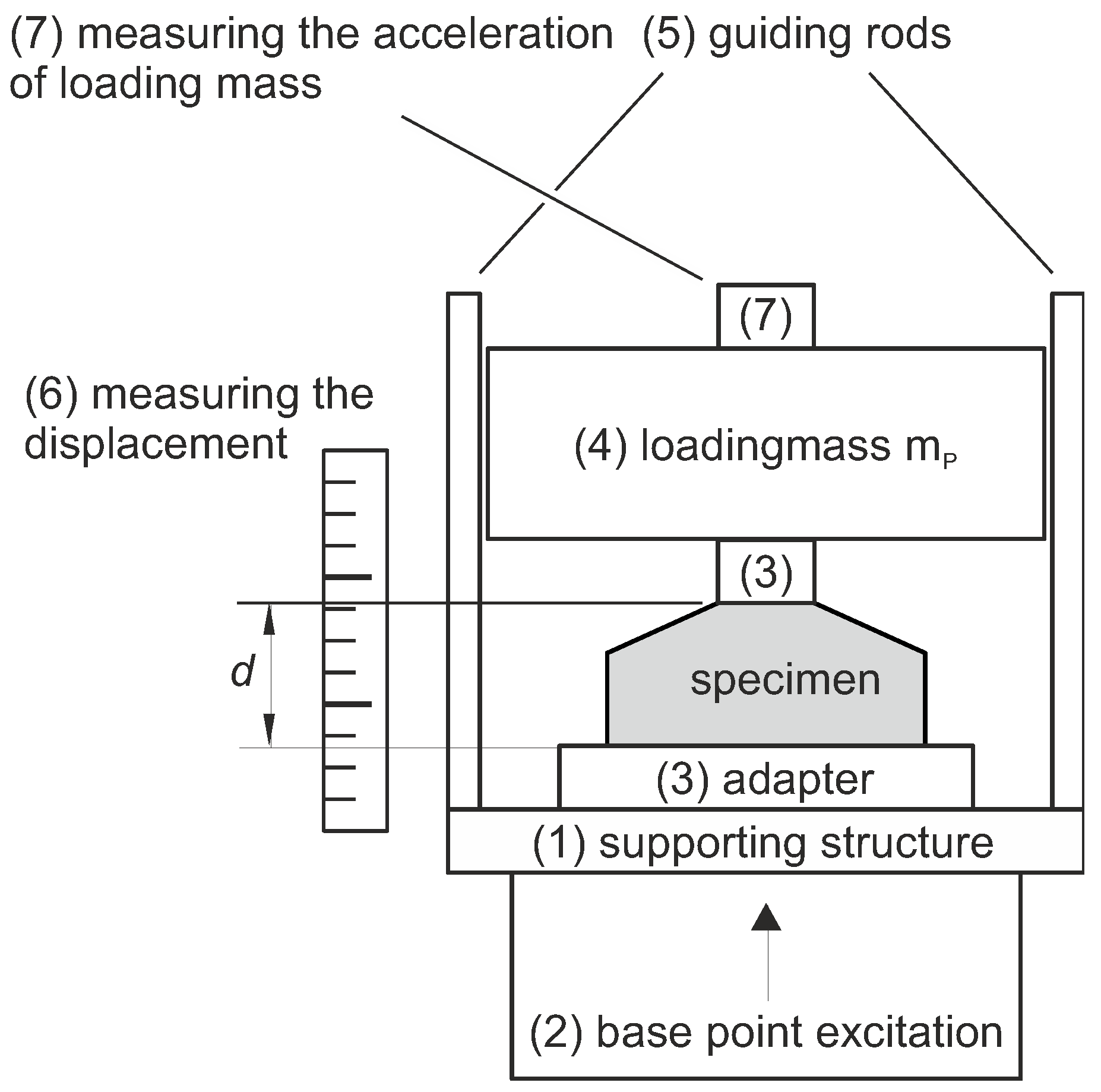
The basic principle of the testbench is shown in Figure 3. Its main components are described in detail after a short overview. A comprehensive description on statistical analysis of acquired data and error considerations can be found in [12].
A vertical shock test machine is used to provide the basepoint acceleration of the shockmount under test. The dynamically generated basepoint acceleration is a haversine-shaped shock pulse. The specimen is mounted on the supporting structure, here the drop table, via measuring adapters. The acceleration of the inert loading mass is measured with an accelerometer, while the displacement of the shockmount is measured by a linear potentiometer. According to Newton’s second law, the restoring force of the shockmount is calculated from the measured acceleration.
2.2.1. Shock Test Machine
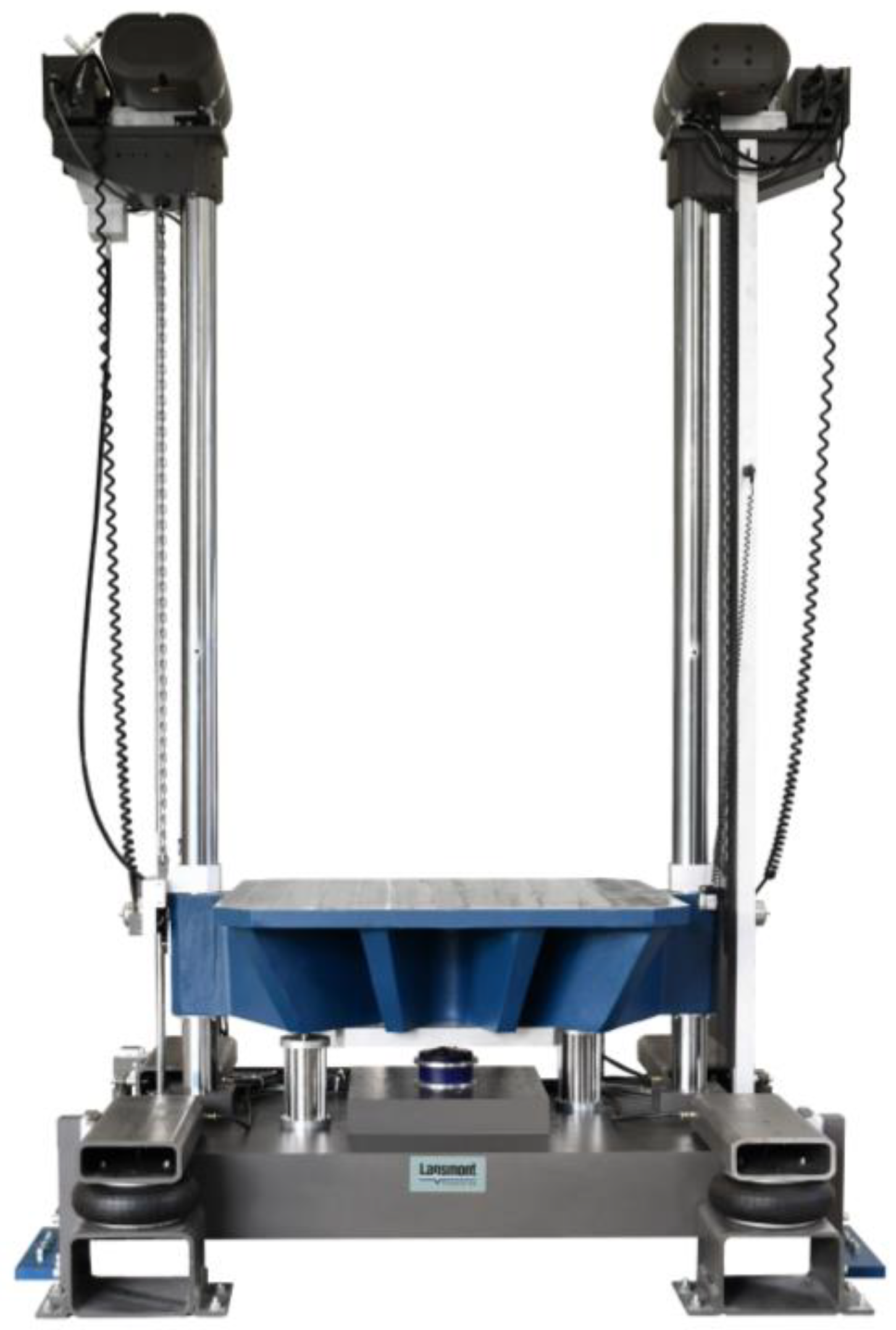
The dynamic shock generation is performed with a free-fall shock test system by the manufacturer, Lansmont Corporation (Monterey, CA, USA), as seen in Figure 4. The specific model is called 122 because of its square shock table with a 122 cm edge length. The system is equipped with a high-capacity option to handle a maximum payload of 1.134 kg on the table. It is mounted on a seismic reaction base, consisting of a heavy steel block that is connected to the floor via airmount-inflated isolators (air springs) in each corner and four shock-absorbing dampers on the left- and right-hand side. The resonant frequency of the seismic base is between 2 and 3 Hz. The horizontal movement of the base is limited by alignment posts.
The drop table is made of aluminum and weighs 635 kg. In order to mount the test specimen, it has a 10 cm square grid hole pattern with M16 × 1.5 inserts. It is guided by round, chrome plated, solid steel rods and can be lifted by chains with two hoist positioning systems.
In addition to the influence of drop height, weight of table, and setup, the shock pulse (g-level, waveform, and duration) can be shaped with devices mounted between the table and the base. Here, a configuration with modular elastomer programmers (MEPs) with cone-shaped faces for haversine [1] shocks and a high dynamic force rating are used. Differing from Figure 4, there are three modules mounted both on the base (2″ thick) and below the table (1/2″ thick).
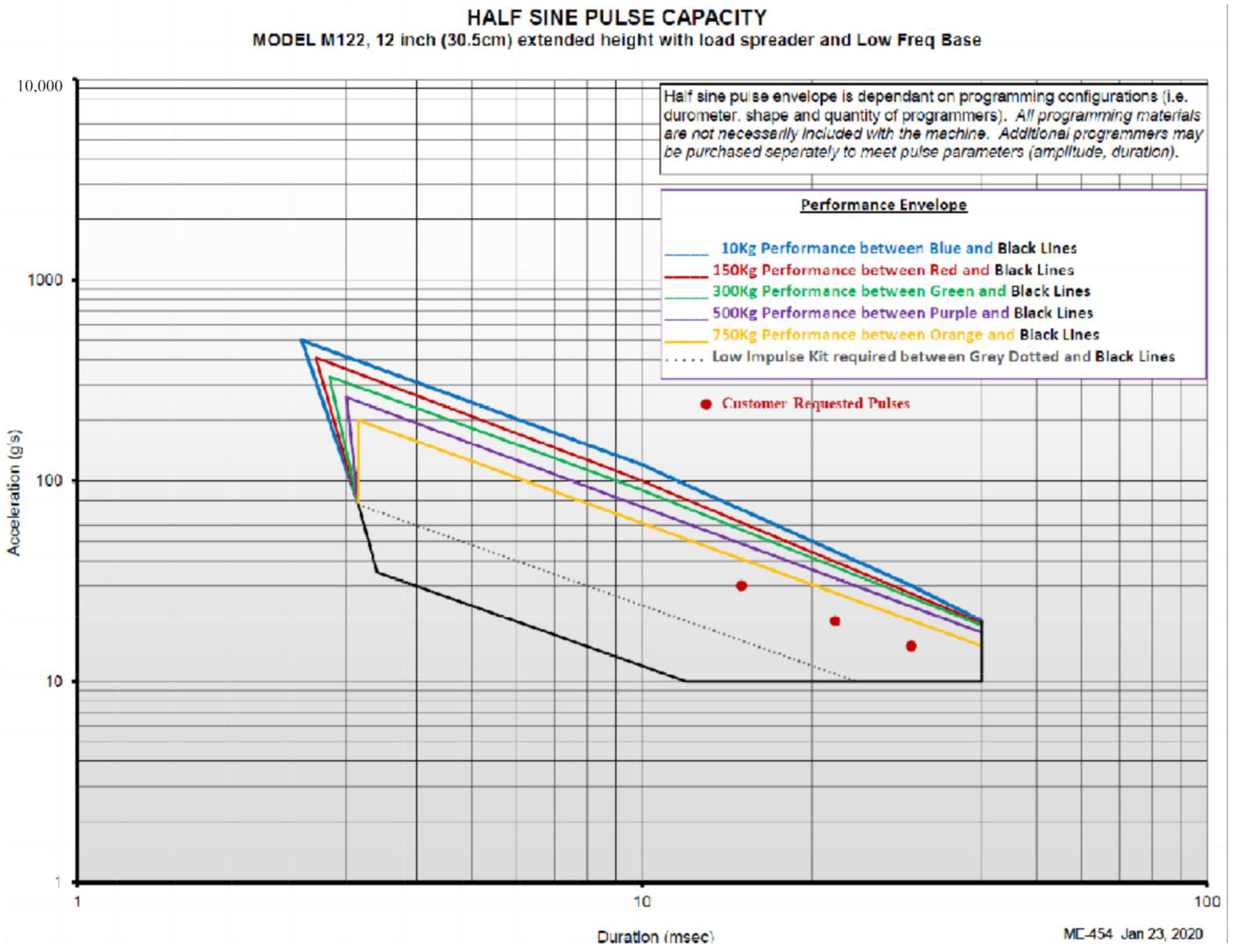
Figure 5 shows the performance limitations of the machine for haversine pulses with polygons in a duration-versus-acceleration-table (DVAT). The manufacturer recommends performing only shocks inside the outlined areas. The maximum acceleration decreases with greater duration and load on the table. The red marks show cases for which the machine was initially used.
2.2.2. Displacement Measuring Devices
For measuring the deformation of the shockmount under test, linear potentiometers of the manufacturer, WayCon Positionsmesstechnik GmbH (Taufkirchen, Germany), type LZW2-A-250-10M, are used, as seen in Figure 6.
The measurement principle of linear potentiometers is based on a potential divider. The linear potentiometer contains a sliding contact running on a resistance track. This sliding contact is fitted with a piston rod which is fixed to the measuring object. As resistance changes proportionally to the actual traversed path by the sliding contact, the distance can be determined by the change in output voltage.
Key features of the used type are:
- Measurement range 250 mm.
- Maximum power supply 60 V
- Displacement speed 10 m/s
- Shock resistance 50 g, 11 ms
- Up to ± 13° tilt
For supplying voltage to the linear potentiometers, signal generators of the data acquisition system with 10 V DC are used. The sensitivity, is the ratio between supply voltage, and maximum displacement, :
2.2.3. Acceleration Sensors
To measure all necessary information about the movement of the loading mass, the shock table, and the seismic base of the shock system, the sensors must cover a wide measuring range and frequency span.
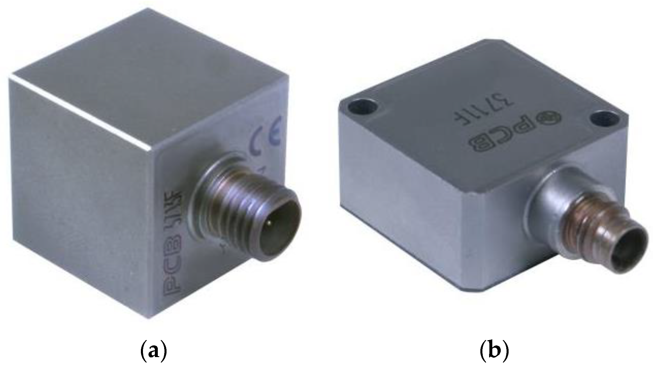
During the drop of the table, the shockmounts underly zero gravity, represented by a constant acceleration that is 1 g smaller than the initial condition with the table at rest. This can only be captured with sensors achieving true DC response. Therefore, MEMS DC accelerometers of the 3710 series (manufacturer: PCB Piezotronics, New York, NY, USA) were chosen. These come in a triaxial (type 3713) and a uniaxial (type 3711) design [19], as seen in Figure 7.
Both designs are specified with a frequency range (5%) from 0 to 1500 Hz. Due to the expected high accelerations under shock (over 100 g), the version F11200G with a measurement range of 200 g peak (sensitivity 6.75 mV/g) was selected [22].
The triaxial type 3713 is mounted with a stud on a prepared thread on the loading mass. The uniaxial type 3711 is screwed to a clip for adhesive mounting, which is fixed with hbm (Hottinger Baldwin Messtechnik) X60 cold curing glue to the supporting structure in order to measure the basepoint acceleration.
The sensors have built-in electronics that are powered by a Model 478A05 three-channel signal conditioner (manufacturer: PCB Piezotronics).
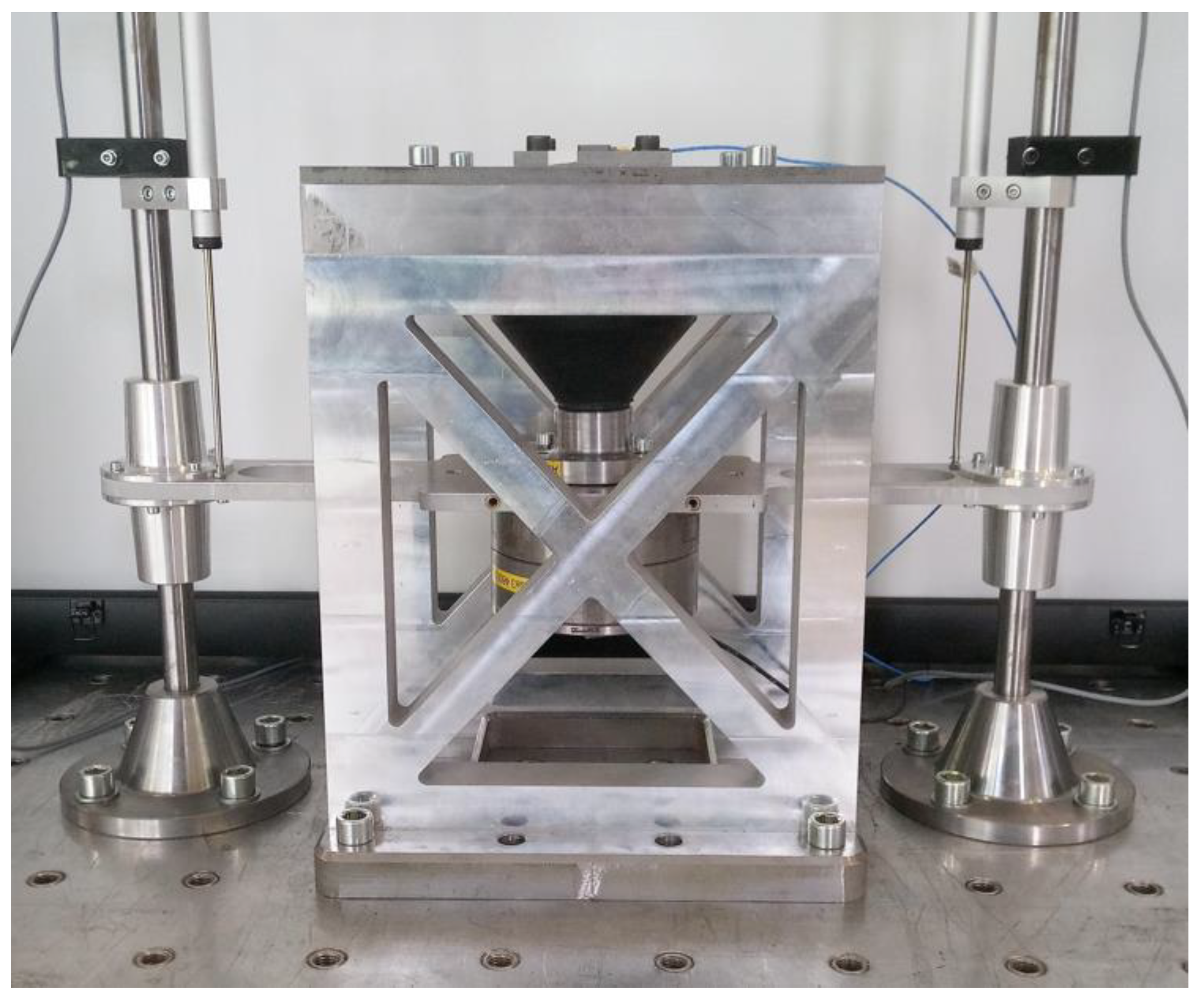
2.2.4. Improved Guiding System and Loading Mass
In order to prevent the shockmount-mass system from tilting and to establish attachment points for the displacement measuring devices, a guiding system is necessary, as seen in Figure 8. The system consists basically of two steel rods, which can be mounted to the drop table, and a horizontal traverse. The traverse is made of aluminum and is connected to the rods by four roller bearings, two at each rod. Also, there are brackets attached to each rod, which fix the linear potentiometers to the system. The piston rods of the linear potentiometers are screwed into threaded holes in the traverse.
Guided by the rods, the traverse can move vertically up and down, as indicated by the double-headed arrow in Figure 8.
The traverse is fitted with threaded holes for attaching the loading mass, the guide adapters, and—in some cases—the wire rope shockmounts (see Section 2.2.5).
In order to meet the required displacements with all shockmount types and load directions, the loading mass has a modular design. It consists of stackable single mass elements with an identical hole pattern and cross-section. With varying thickness, mass elements of 1 kg, 2 kg, and 5 kg are used. Figure 9 shows a 5 kg element.
This guiding system has been improved with respect to the system used in the original work reported in [12]. It is sturdier, more versatile, and easier to handle when changing the specimen is necessary. The basic principle is the same; however, the original roller bearings were replaced by plain bearing bushes. For this reason, the dynamic model and some equations have to be adapted. Friction in the bearings can be neglected, and there is no moment of inertia in the bearings anymore.
Thus, the quantities, and , from Equations (7), (15) and (28) in [1], which represent the mass of the rollers in the bearing and its maximum uncertainty, are set to zero. The quantity, in these equations includes the loading mass as well as the mass of the horizontal traverse and of the bearings.
2.2.5. Measuring Adapters
In order to establish measurement setups that allow for the load directions of both shockmount types as defined in Figure 2, several measurement adapters were designed. They were manufactured by HSU (Helmut Schmidt University) central workshop. All seven possible configurations are shown for clarity in Section 2.2.6.
Basepoint adapters (Figure 10) are used to mount the shockmount to the drop table and therefore transmit the shock pulse. Guide adapters (Figure 11), however, connect the shockmount to the traverse of the guiding system. Therefore, they are on the shock-isolated side of the system.
Wire rope shockmounts in pressure-, tension-, and roll-configurations do not need a guide adapter since they are connected directly to the traverse of the guiding system.
The adapters are mainly drilling and milling parts and, with two exceptions, are made of steel. The basepoint adapter for tension configuration (Figure 10b) has a steel base, while the walls and the lid are made from high-strength aluminum. The guide adapter for wire rope shockmounts in shear configuration (Figure 11c) is made of aluminum in order to reduce weight.
2.2.6. Complete Setup
In this section, for every possible configuration, a sketch and a picture of implementation are given:
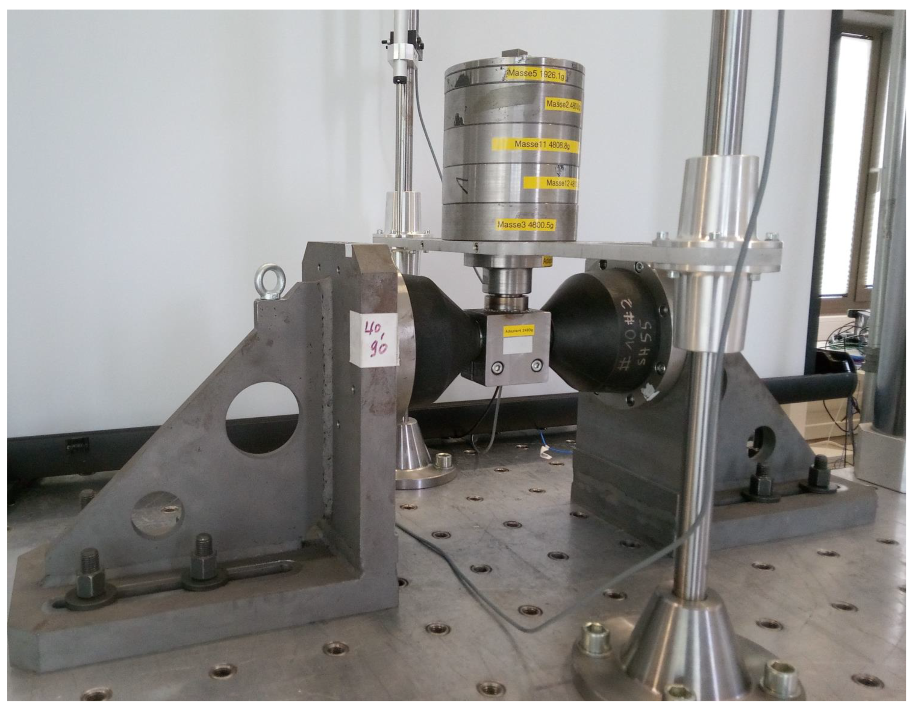
For all configurations, due to the guiding system, the loading mass and the interface of the shockmount can move only vertically, together with the connected traverse. This is illustrated by the double-headed arrow in Figure 12 for elastomer shockmounts in pressure configuration.
The cubic elements shown in the sketches represent the accelerometers.
2.2.7. Highspeed Camera
To monitor the shock tests, a highspeed camera by the manufacturer, Phantom Ametek (Wayne, NJ, USA), type VEO 710S, is used together with 2 LED spots, as seen in Figure 26. Even though the camera is capable of acquiring videos with up to 690,000 frames per second at lower resolution, here, the sample rate is chosen to be 3000 frames per second, with a resolution of 1280 × 800 pixels. This is sufficient to capture the exact moment of distinct states, such as maximum negative and positive displacement.
2.2.8. Data Acquisition
For acquiring time data of the sensor signals, LAN-XI modules by the manufacturer, Brüel & Kjær (Nærum, Denmark), are used. The measured data are analyzed with the belonging software, PULSE LabShop, in version 25.
Distributed over three modules, nine signals are measured, as listed in Table 2.
Data acquisition was carried out with an FFT Analyzer, recording time blocks and computing spectra. Along with FFT setup parameters for a frequency span from 0 Hz to 3.2 kHz, the analog signals were digitized with a sample frequency 2.56 times higher, leading to a sample time of 122.07 µs. Along with a spectral resolution of 6400 lines, time blocks are 2 s long. Recording was triggered with an instrument trigger signal (InstTrig), generated by the shock system, beginning 0.6 s before trigger signal starts.
In Figure 27, acceleration signals are shown exemplarily for acceleration sensors on the basepoint (a2_z) and seismic base of the shock test machine to show a typical run. The data come from a measurement with a wire rope shockmount under compression with a drop height of 65 cm. Beginning shortly after 0.2 s, the table drops, and the value of the accelerometer, a2_z, also does, staying at a lower level. After 0.6 s, the accelerometer signals measuring in the vertical direction have a short peak, followed by a decay with high-frequency components. The peak of the seismic base sensor is oriented opposite to the peak of the basepoint sensor, since the elastic impact of the table to the base causes downward movement of the seismic base.
Figure 28 shows in detail the time range before the impact. Now, the shift of basepoint acceleration, a2_z, can be read as about −10 m/s2. The value of the sensor at the start of the time record is not zero or 1 g, due to an offset in the signal conditioner. Signal a1_z (mounted on loading mass) has a shift in the positive direction because it is inverted. Signal inversion is conducted so that negative acceleration and, therefore, negative force values are obtained at the compression of the shockmount, which is the convention in force-displacement characteristics. Thus, the results will be presented in accordance with the sign convention.
The value of the sensor at the base rises a little due to the relaxing of its air spring support under lower overall weight. It also can be seen that the noise of sensors a2_z and aBase_z is lower: these signals are measured with uniaxial accelerometers, where a1_z is a triaxial one, having higher inherent noise. Since measured data get lowpass-filtered for further use [12], this noise is reduced to a level where all relevant features of motion can be evaluated.
The programmers of the table and base begin to touch at t = 0.613 s, as seen in Figure 29. The basepoint sensor has a haversine shape with a length of about 12 ms. The shock pulse is followed immediately by a high-frequency signal, which reflects the vibration modes of the drop table.
Again, the values measured at the base oppose, as it is pushed downwards by the impact of the table.
The acceleration signal, a1_z, measured on the loading mass is a highly damped, nonlinear oscillation without a distinct time period, as seen in Figure 30. The data of linear potentiometers for measuring displacement of the shockmounts follow the acceleration at the loading mass, but it is smoother with less high-frequency components, as can be seen in Figure 31.
2.2.9. Reproducibility
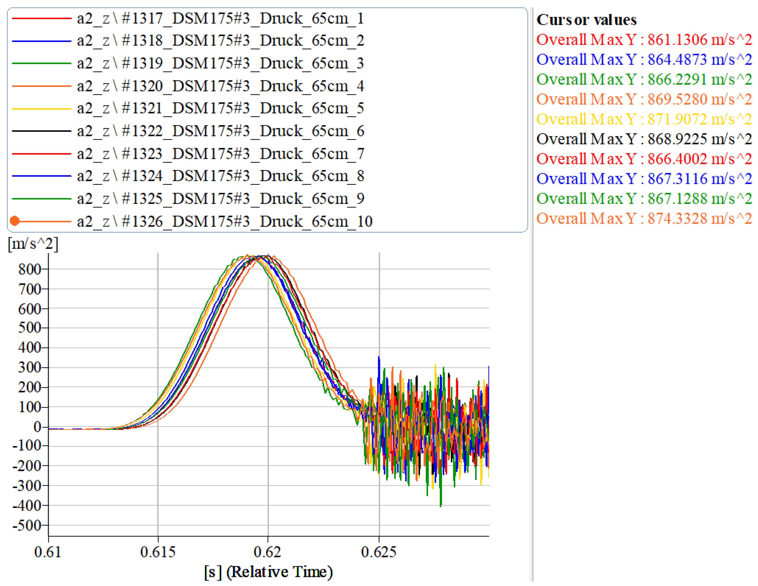
The shock conditions are highly reproducible, as can be seen in Figure 32.
The shapes of all 10 runs shown in the figure are nearly identical. The time shift of the basepoint excitation reveals the varying trigger times. Since the coherent data acquisition of loading mass acceleration and displacement is started by the same trigger, the inaccuracy of the trigger signal has no effect on the accuracy of the measurements.
The absolute deviation between the largest and the smallest overall maximal values is under 1.5%. The maxima have a tendency of rising with the run number, as seen in Figure 33.
2.3. Advanced Kelvin–Voigt Model and Parameter Identification
One of the use-cases for the described setup is to generate force-displacement data of the shockmounts, from which parameters for a simulation model can be derived.
The advanced Kelvin–Voigt model, as introduced in [14], has good agreement for elastomer shockmounts and—if the parameters are properly determined—within the first two cycles of decay for wire rope shockmounts. Because this is the regime of interest in terms of shock response, this model is suitable to describe the dynamic behavior of shockmounts sufficiently.
The advanced Kelvin–Voigt model is a basic model describing the shockmount as a nonlinear spring with stiffness parameters, , in parallel to a viscous damper with a constant damping coefficient, b. The relation between restoring force, and displacement, is given by:
For simulation purposes, the equation of motion for the displacement, of the shockmount is:
where is the inert loading mass that deforms the shockmount. is the basepoint acceleration and can be taken from the measurement.
The damping and stiffness parameters, , of the model are identified with regard to the properties of a single-mass oscillator (of mass M).
Figure 34 shows exemplary experimental force-displacement-hysteresis behavior for the first cycle of oscillation in a measurement for a wire rope shockmount (drop height ). The force curve, (blue), proceeds from the maximum tension to the maximum compression data point and (red), vice versa. The force curve, , in Figure 33 is the mean value result of and . It represents the conservative, nonlinear force-displacement characteristics of the shockmount. The enclosed area is a measure of the amount of energy dissipation caused by damping [12].
2.3.1. Non-Linear Spring Force
2.3.2. Damping Coefficient
For viscous damping, the damping coefficient, can be substituted by the dimensionless equivalent damping ratio, , with:
With the undamped circular eigenfrequency , this equation can be modified to:
The stiffness coefficient, and the viscous damping ratio, are derived from experimental results.
For calculating the damping ratio out of force-displacement hysteresis, Equation (6) can be used [12]:
There, and are the span of the measured displacement and the measured force values. is the amount of energy dissipation caused by damping. It is represented by the enclosed area of the hysteresis loop (Figure 34). This energy is computed numerically in MATLAB by stepwise trapezoid area procedure.
From Figure 31, it is obvious that damping in wire rope shockmounts is not, in fact, constant. Therefore, the damping coefficient, is valid only in the range of the first cycle, from which the damping ratio is obtained. This is the reason why the advanced Kelvin–Voigt model yields good results only in the first few cycles for wire rope shockmounts.
For the equivalent stiffness coefficient, , a linear approach is chosen with the purpose of calculating the constant damping coefficient in Equation (5). It is obtained by:
With Equations (6) and (7), all necessary quantities are known to calculate the damping coefficient. The parameters are listed in Table 4.
2.4. Simulation
2.4.1. State Vectors
The dynamic model (3) is implemented in MATLAB to solve ordinary differential equation problems (ODEs) in the time domain. Since a nonlinear term is included with the 5th order polynomial spring force, an analytical solution for the ODE is difficult to find. Alternatively, a numerical procedure for solving initial value problems can be utilized here [23]. In general, ODEs of second order (or more) have to be interlaced in several state vectors of the first order.
Exemplarily, the state vector
contains the displacement, and velocity, , while its time derivative
is consequently structured in the velocity, and acceleration, corresponding to (3). By proposing an initial state vector , the solver system is able to compute the derived state vector, as a slope to determine the following state vectors stepwise. Therefore, this state representation is well adapted to the dynamic problem.
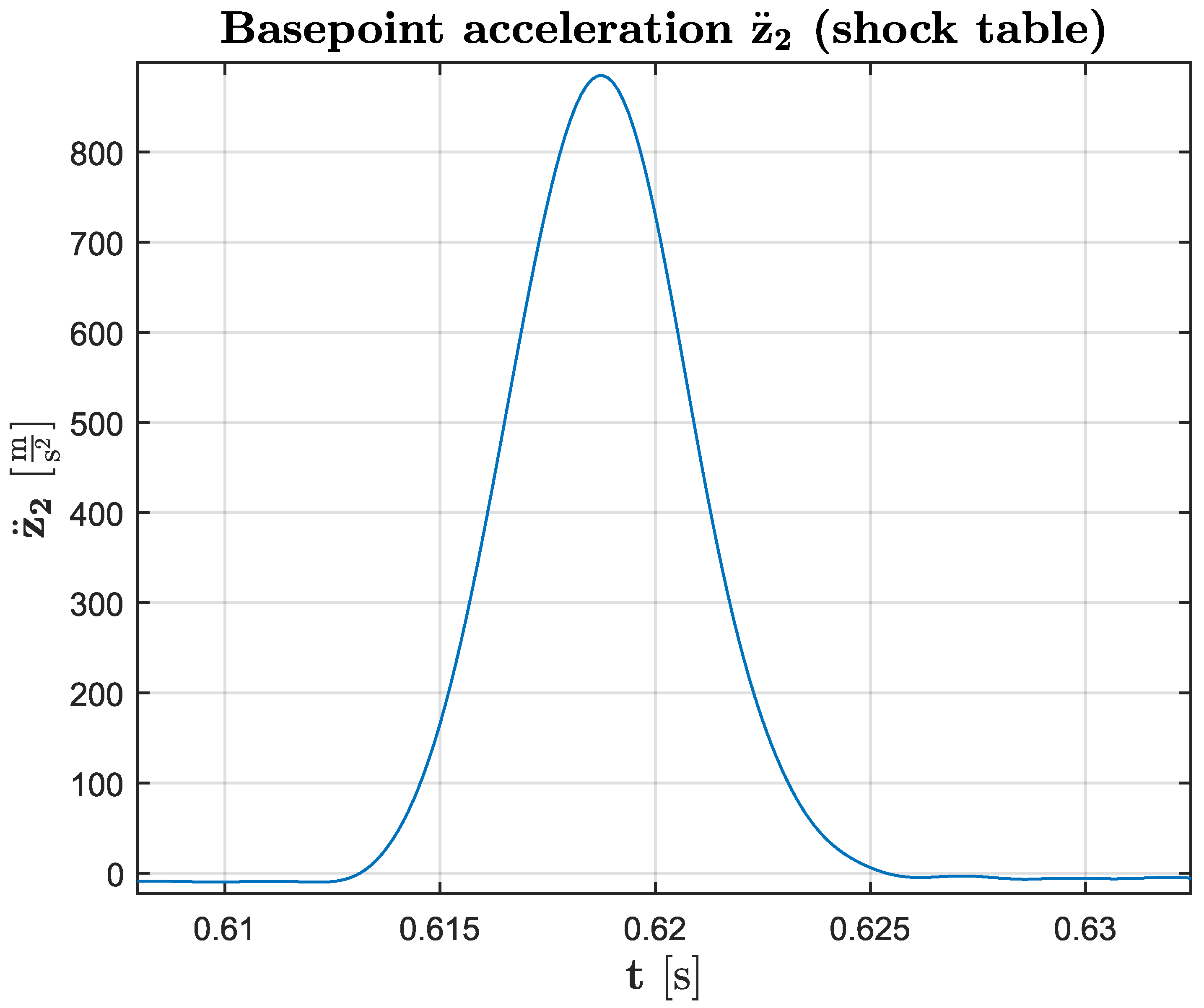
2.4.2. Basepoint Excitation
The impact on the dynamic model is given by base point excitation, which is a dataset of the acceleration measurements, , of the drop table. The main excitation happens in the time span of s, while the acceleration peak occurs at s with a magnitude of , as seen in Figure 35.
Immediately after this haversine excitation, the brake system of the shock testbench is activated, and the acceleration rapidly tends towards .
It is important to mention that the amount and step size of and between the data points should match with the number and increment of the state vectors of the numerical solution.
2.4.3. Numerical ODE45 Solver in MATLAB
In the following section, the main proceedings of programming the simulation in MATLAB are explained by means of Figure 36.
First, the initial value problem requires a start state vector, x_start. In this case, it can be assumed that the displacement as well as the velocity of the SM at s (shortly before the shock impact) are neglectably small. Nevertheless, for consistent handling, measurement data can be read in here. Second, the time vector, t_span, for the numerical solution is chosen to coincide with the length of the time vector related to the dataset, of the base point acceleration measurements. Third, the ODE45-solver for the simulation is formulated. It is based on the numerical Runge–Kutta method of 4th order with an estimated error of 5th order. Beginning from x_start, the stepsize within every iteration shall be taken from the increment of t_span.
Finally, the time-derived state vector of (9) shall be declared in a function, called odefun here, which communicates with the ODE45-solver. It is fed by a list of parameters, i.e., the damping coefficient b, the stiffness coefficients p = [k5, k4, k3, k2, k1, k0] (Table 3 and Table 4), and the dataset . Within every iteration, the actual state vector of (8) is requested to compute the instantaneous spring force from the nonlinear function, F_k. Furthermore, the actual base point acceleration, a2 (scalar format), shall be taken from the dataset. This is realized by the interp1 function, taking the interpolated value of z2pp at every time point, t, within t2pp.
All of the above-mentioned quantities are utilized to compute the time-derivative of the state vector of (9) for every iteration step in the ODE45 algorithm. The solution consists of multiple data pairs in the form of the state vector, ].
3. Results and Discussion
3.1. Testbench
A series of about 2000 measurements with all combinations of shockmount types and loading orientations and drop heights was conducted. The obtained datasets are useful to generate dynamic force-displacement characteristics, as reported in [12].
They are also sufficient to gain parameters for the advanced Kelvin–Voigt model, as shown in the following subsections. The measurements and the parameters obtained from them confirm the robustness of the advanced Kelvin–Voigt model within the described limitations.
Despite the very good overall usability of the testbench, several aspects should be mentioned:
- The horizontal traverse of the guiding system, including the housings of the plain bearing bushes, contribute to the loading mass that loads the shockmount. For very soft shockmounts, such as the WSM 175 in shear or roll configurations, almost no additional loading mass is required to displace the shockmount dynamically. In these cases, the mass of the traverse should be as small as possible. Nevertheless, the stiffness of the traverse must be high enough to prevent the bearing housings from oscillating around the middle of the traverse.
- Even if the linear potentiometers in the proposed setup are attached to the guiding traverse, the displacement could be measured, for example, by non-contact evaluation of highspeed camera images. However, the guiding system is required to prevent shockmount-mass combination from tilting. This is especially true for configurations with wire rope shockmounts, which usually show an asymmetric construction, or for configurations with a high center of gravity when using multiple stacked mass modules.
- The linear potentiometers for measuring the displacement have a specified shock capability of only 50 g at 11 ms. In the conducted measurement series, basepoint excitations up to 165 g at 10 ms were applied. As long as the potentiometers were loaded axial to the piston rod, they showed good usability without any failure.
- The intention for using triaxial accelerometers for measuring acceleration of the loading mass was to observe if there is motion of the loading mass in the two directions orthogonally to excitation. Evaluation of measurements showed that there is no significant motion in these directions.
Finally, during the performance of the measurement series, it turned out that the described testbench is very well suited for measuring the force-displacement characteristics for wire rope shockmounts as well as for elastomer shockmounts. If shockmount models other than those used here are to be measured, the measuring adapters must be fitted to the specific shockmount type.
3.2. Exemplary Simulation
In this section, the results from the simulation for the exemplary wire rope shockmount, as described in Section 2.4, are presented and compared to those of the measurements. In Figure 37, the time diagram of the relative displacement is introduced.
The simulation results are in good agreement with the measurement results for the first two cycles. Beyond this, as expected, the simulation results reveal a longer decay process with nine cycles of oscillation due to the assumption of a velocity-dependent quasi-viscous damping ratio. In the measurement results, the dry friction damping influence of the wire rope shockmount is more effective, so the decay process takes only three cycles of oscillation, while a static displacement of 9 mm remains due to adherence forces within the shockmount.
In Figure 38, the time diagram of the relative acceleration is presented. At s, the shock mount system reacts to the basepoint excitation of the shock table with
Again, measurement and simulation results are in good agreement for the first two cycles of oscillation. Beyond this, the decay process of the simulation results takes longer than that of the measurement results.
Figure 39 shows the first loop of the force-displacement-diagram. The good agreement concerning the hysteretic behavior of simulation and measurement results is visible, since the load and unload curves form the typical area of energy dissipation caused by damping.
At and the hysteretic areas of the simulation results have a slimmer shape than those of the measurement results. This is due to the viscous, velocity-dependent damping force of the model, which is relatively small near the turning points from load to unload, or vice versa, where the velocity changes its direction.
Figure 40 illustrates the complete hysteretic behavior of the restoring force (simulation and measurement) with the long-term constriction due to the decaying oscillation.
Obviously, the simulation result has more hysteresis loops than the measurement result, which again means that the decay process takes longer in the simulation.
Finally, Figure 41 shows the nonlinear spring force diagram where the mean values of the measured load and unload curves are in good agreement with the computed spring force from the simulation results.
3.3. Parameter Sets for the Advanced Kelvin–Voigt Model
Several combinations of shockmount type, specimen, loading orientation, and drop height are selected. This selection is exemplary and reflects the wide bandwidth of possible combinations, as well as the robustness previously shown. Table 5 gives an overview and presents the associated parameter sets for the advanced Kelvin–Voigt model.
While the drop height influences the velocity change of the shockmount, the combination of drop height and loading mass always is chosen such that the maximum specified displacement is obtained.
For each of the exemplary configurations, the measured force-displacement characteristics, together with the simulated curve, are included in Appendix A, similar to Figure 41. Inspection of these curves shows that for elastomer shockmounts, the coefficient of determination is within a three-digit precision, and for wire rope shockmounts, . This shows a very good agreement from simulation to measurement and indicates that the advanced Kelvin–Voigt model for both shockmount types, together with its gained parameters, is suitable for further usage.
4. Conclusions
Concluding the study, there are three main points:
The proposed setup is versatile for investigating wire rope shockmounts and elastomer shockmounts. The measurement data are not only suitable for calculating the force-displacement characteristics of the shockmounts under test but also for identifying their parameters for the advanced Kelvin–Voigt model. The advanced Kelvin–Voigt model, together with the parameter sets identified from measurement data, yields a good representation of the dynamic behavior of the specific shockmounts. For wire rope shockmounts, this applies only in the limited range of the first one to two oscillations after shock excitation.
This study is focused on shockmounts with elastic deformation. One of many open perspectives for the inertia-based approach and this setup is the investigation of the dynamic behavior of shockmounts with plastic deformation. With minor modification, the dynamic force-displacement characteristics of yielding straps and crash elements from the automotive or aviation field can be determined.
Author Contributions
Conceptualization, B.H., K.S., M.C., J.D. and D.S.; methodology, B.H. and D.S.; software, B.H. and M.C.; validation, B.H., K.S., M.C. and D.S.; resources, K.S. and B.H.; writing—original draft preparation, B.H., K.S. and M.C.; writing—review and editing, B.H., K.S., M.C. and D.S.; visualization, B.H., K.S. and M.C.; supervision, D.S.; project administration, D.S., J.D. and B.H.; funding acquisition, B.H. All authors have read and agreed to the published version of the manuscript.
Funding
This work was funded by the German Bundeswehr Technical Center for Ships and Naval Weapons, Maritime Technology and Research (WTD 71).
Data Availability Statement
Data will be made available on request.
Acknowledgments
The authors express their appreciation and gratitude to their colleagues, Holger Beneke, who has constructed the measuring adapters and the improved guiding system, and Tom Langmann, who supported almost every phase of the project.
Conflicts of Interest
The authors declare no conflict of interest. The funder had a consulting role in the design of the study and—since it has a military background—gave permission to publish the results.
Appendix A
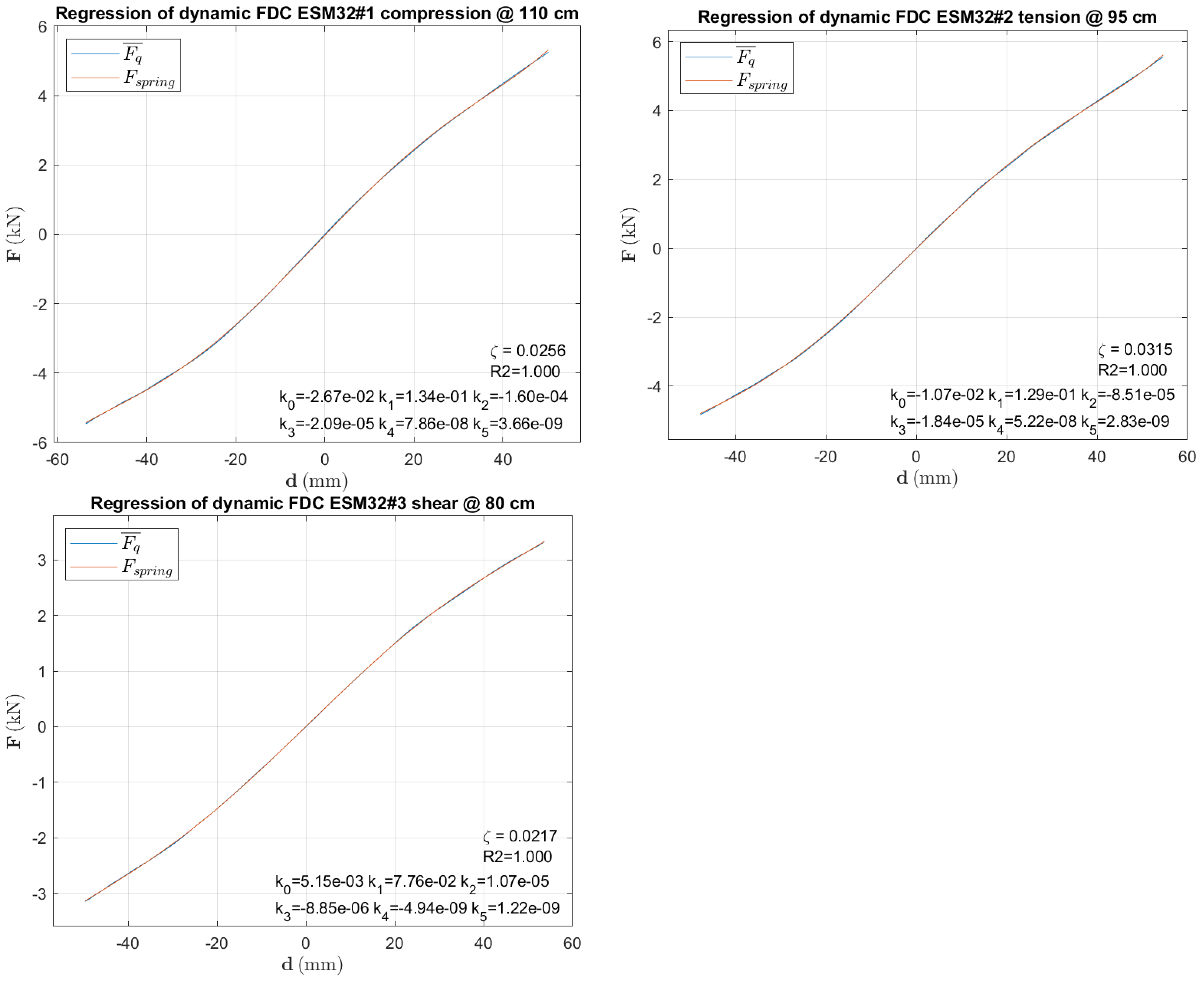
The curves presented here are the calculated (red lines) and measured (blue lines) force-displacement characteristics (FDCs) of the selected shockmount-load combinations. The headings of the printouts reveal the combination:
- Shockmount type (ESM32, ESM40, ESM 55, WSM125, WSM135, WSM175, according to Section 2.1)
- Specimen number (#1, #2, #3) out of three specimens of a shockmount type
- Load directions (compression, tension, shear, roll)
- Drop height (in cm)
In addition to the curves, the damping ratio, and the stiffness parameters are shown.
Appendix A.1. Elastomer Shockmounts

Appendix A.2. Wire Rope Shockmounts


References
- Sisemore, C.; Babuska, V. The Science and Engineering of Mechanical Shock, 1st ed.; Imprint; Springer International Publishing: Cham, Switzerland, 2020. [Google Scholar]
- Akram, P.A.; John, B.M.; Madathil, T.S.; Shija, C.; Abhirami, P.; Mathiazhagan, A.; Tide, P.S.; Ebenezer, D.D. Numerical Model of a Multi-layer Shock and Vibration Isolator. In Proceedings of the OCEANS 2022, Chennai, India, 21–24 February 2022; pp. 1–6. [Google Scholar]
- Prost, C.; Abdelnour, B. Influence and Enhancement of Damping Properties of Wire Rope Isolators for Naval Applications. Sound Vib. 2018, 52, 1–4. [Google Scholar] [CrossRef]
- Zhang, C.; Lu, K.; Zhang, L.; Yan, M.; Zhang, Y. Experimental study on mechanical properties of new biaxial compression wire rope isolator. Sci. Sin.-Phys. Mech. Astron. 2021, 51, 124612. [Google Scholar] [CrossRef]
- Grządziela, A.; Kluczyk, M. Shock Absorbers Damping Characteristics by Lightweight Drop Hammer Test for Naval Machines. Materials 2021, 14, 772. [Google Scholar] [CrossRef] [PubMed]
- Kluczyk, M.; Grządziela, A.; Pająk, M.; Muślewski, Ł.; Szeleziński, A. The Fatigue Wear Process of Rubber-Metal Shock Absorbers. Polymers 2022, 14, 1186. [Google Scholar] [CrossRef] [PubMed]
- Mannacio, F.; Barbato, A.; Di Marzo, F.; Gaiotti, M.; Rizzo, C.M.; Venturini, M. Shock effects of underwater explosion on naval ship foundations: Validation of numerical models by dedicated tests. Ocean. Eng. 2022, 253, 111290. [Google Scholar] [CrossRef]
- Wang, Y.; Dong, H.; Dong, T.; Xu, X. Dumbbell-Shaped Damage Effect of Closed Cylindrical Shell Subjected to Far-Field Side-On Underwater Explosion Shock Wave. J. Mar. Sci. Eng. 2022, 10, 1874. [Google Scholar] [CrossRef]
- Gargano, A.; Mouritz, A.P. Comparative study of the explosive blast resistance of metal and composite materials used in defence platforms. Compos. Part C Open Accesss 2023, 10, 100345. [Google Scholar] [CrossRef]
- DIN 95415:2020-11; Drahtseil-Federelemente—Technische Spezifikation. Deutsches Institut für Normung e.V.: Berlin, Germany, 2020.
- DIN 95360:2009-06; Elastomer-Federelemente—Technische Spezifikation. Deutsches Institut für Normung e.V.: Berlin, Germany, 2009.
- Heinemann, B.; Dreesen, J.; Sachau, D. Dynamic measuring of force-displacement-characteristics of shockmounts. Heliyon 2023, 9, e16743. [Google Scholar] [CrossRef] [PubMed]
- ANEP 63; Shock Mount Characterisation NATO Naval Armaments Group NG6/SG7 on Ship Combat Survivability. NATO: Washington, DC, USA, 2001.
- Clasen, M.; Sachau, D. Simulation models investigating the dynamic characteristics of shock isolators. Proc. Appl. Math. Mech. 2023, 22, e202200017. [Google Scholar] [CrossRef]
- Willbrandt, K.G. (Ed.) CAVOFLEX Drahtseil-Federelemente, Product Catalogue. Available online: https://www.willbrandt.com/willbrandt/en/imprint/imprint.php?test=1 (accessed on 29 September 2023).
- Willbrandt, K.G. (Ed.) Schockdämpfer: Produkte—Daten-Anwendungen, Product Catalogue. Available online: https://www.willbrandt.de/willbrandt/de/schwingungstechnik/schockdaempfer_SES6000.php (accessed on 29 September 2023).
- Lansmont Corporation (Ed.) Half Sine Pulse Capacity: Model M122, 12 inch (30.5 cm) Extended Height with Load Spreader and Low Frequency Base; Lansmont Corporation: Monterey, CA, USA, 2020. [Google Scholar]
- WayCon Positionsmesstechnik GmbH (Ed.) Linearpotentiometer: Serie LZW2; WayCon Positionsmesstechnik GmbH: Taufkirchen, Germany, 2020. [Google Scholar]
- PCB Piezotronics (Ed.) 3710 Series DC Accelerometer Operating Guide; PCB Piezotronics: Depew, NY, USA. Available online: https://www.pcbpiezotronics.fr/wp-content/uploads/3713f1250g.pdf (accessed on 29 September 2023).
- PCB Piezotronics. 3713F11—Online Photo. Available online: https://www.pcb.com/contentStore/images/pcb_corporate/vibration/products/photo/400/3713f11.jpg (accessed on 5 August 2022).
- PCB Piezotronics. 3711F11—Online Photo. Available online: https://www.pcb.com/contentStore/images/pcb_corporate/vibration/products/photo/400/3711f11.jpg (accessed on 5 August 2022).
- PCB Piezotronics (Ed.) Triaxial DC Response Accelerometer: Model 3713F11200G; Spec 70528; PCB Piezotronics: Depew, NY, USA, 2019. [Google Scholar]
- Shampine, L.; Reichelt, M. The MATLAB ODE Suite. SIAM J. Sci. Comput. 1997, 18, 1–22. Available online: https://www.mathworks.com/help/pdf_doc/otherdocs/ode_suite.pdf (accessed on 29 September 2023). [CrossRef]
Figure 1.
Investigated wire rope shockmounts (a) and elastomer shockmounts (b), one of each type.


Figure 3.
Basic principle of the testbench [12].
Figure 3.
Basic principle of the testbench [12].

Figure 4.
Front view of the shock system (photo: Media Center, HSU).

Figure 5.
Performance chart of the shock system [17].
Figure 5.
Performance chart of the shock system [17].

Figure 6.
Linear potentiometer, in the middle of the used model A [18].
Figure 6.
Linear potentiometer, in the middle of the used model A [18].
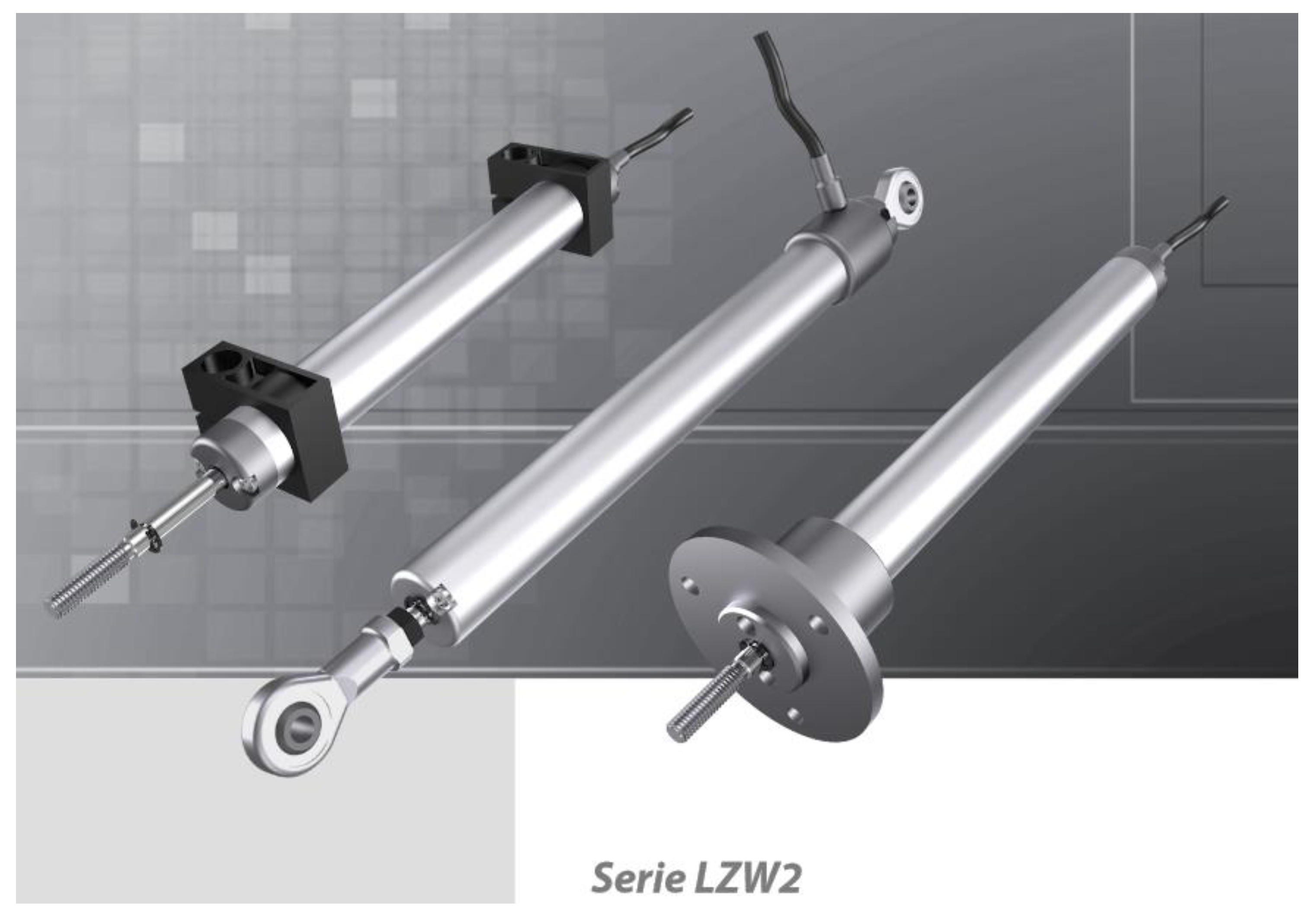

Figure 8.
Improved guiding system.

Figure 9.
Mass element with threaded and unthreaded holes for stacking and attaching other elements, e.g., accelerometer.
Figure 9.
Mass element with threaded and unthreaded holes for stacking and attaching other elements, e.g., accelerometer.
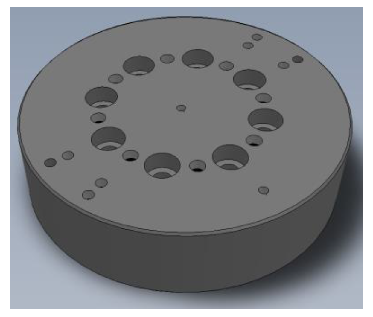
Figure 10.
Basepoint adapters for mounting the shockmount to the drop table for both elastomer and wire rope shockmounts: (a) for configurations in compression mode; (b) for configurations in tension mode; (c) for configurations in shear and roll mode.
Figure 10.
Basepoint adapters for mounting the shockmount to the drop table for both elastomer and wire rope shockmounts: (a) for configurations in compression mode; (b) for configurations in tension mode; (c) for configurations in shear and roll mode.

Figure 11.
Guide adapters for mounting the shockmount to the guiding system: (a) for elastomer shockmounts in compression and tension configurations; (b) for elastomer shockmounts in shear configuration; (c) for wire rope shockmounts in shear configuration.
Figure 11.
Guide adapters for mounting the shockmount to the guiding system: (a) for elastomer shockmounts in compression and tension configurations; (b) for elastomer shockmounts in shear configuration; (c) for wire rope shockmounts in shear configuration.

Figure 12.
Sketch of elastomer shockmount in pressure configuration.

Figure 13.
Picture of elastomer shockmount in pressure configuration.

Figure 14.
Sketch of wire rope shockmount in pressure configuration.
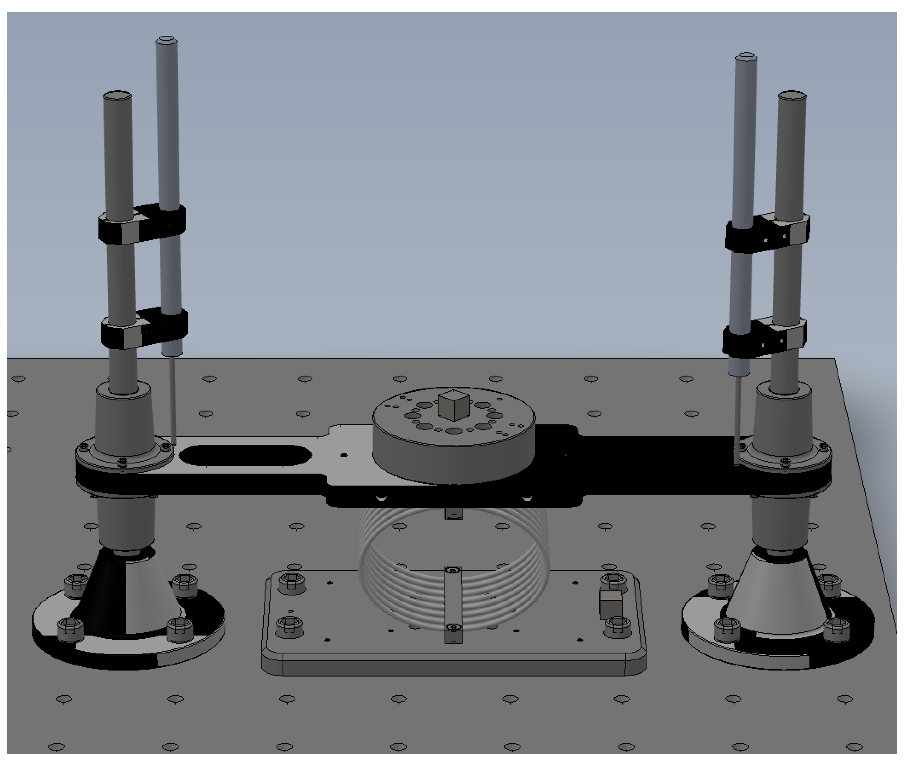
Figure 15.
Picture of wire rope shockmount in pressure configuration.

Figure 16.
Sketch of elastomer shockmount in tension configuration.

Figure 17.
Picture of elastomer shockmount in tension configuration.

Figure 18.
Sketch of wire rope shockmount in tension configuration.

Figure 19.
Picture of wire rope shockmount in tension configuration.
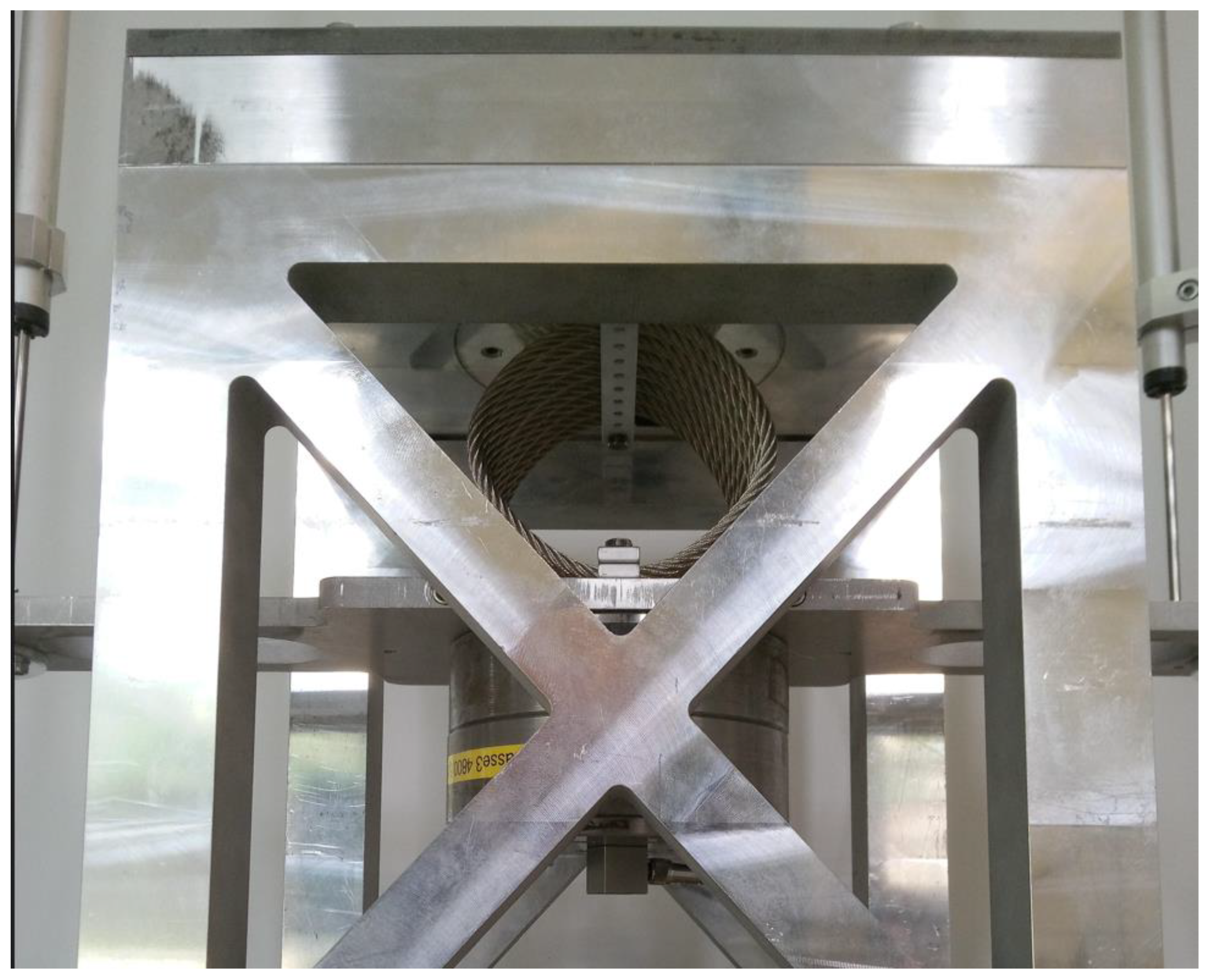
Figure 20.
Sketch of elastomer shockmounts in shear configuration.
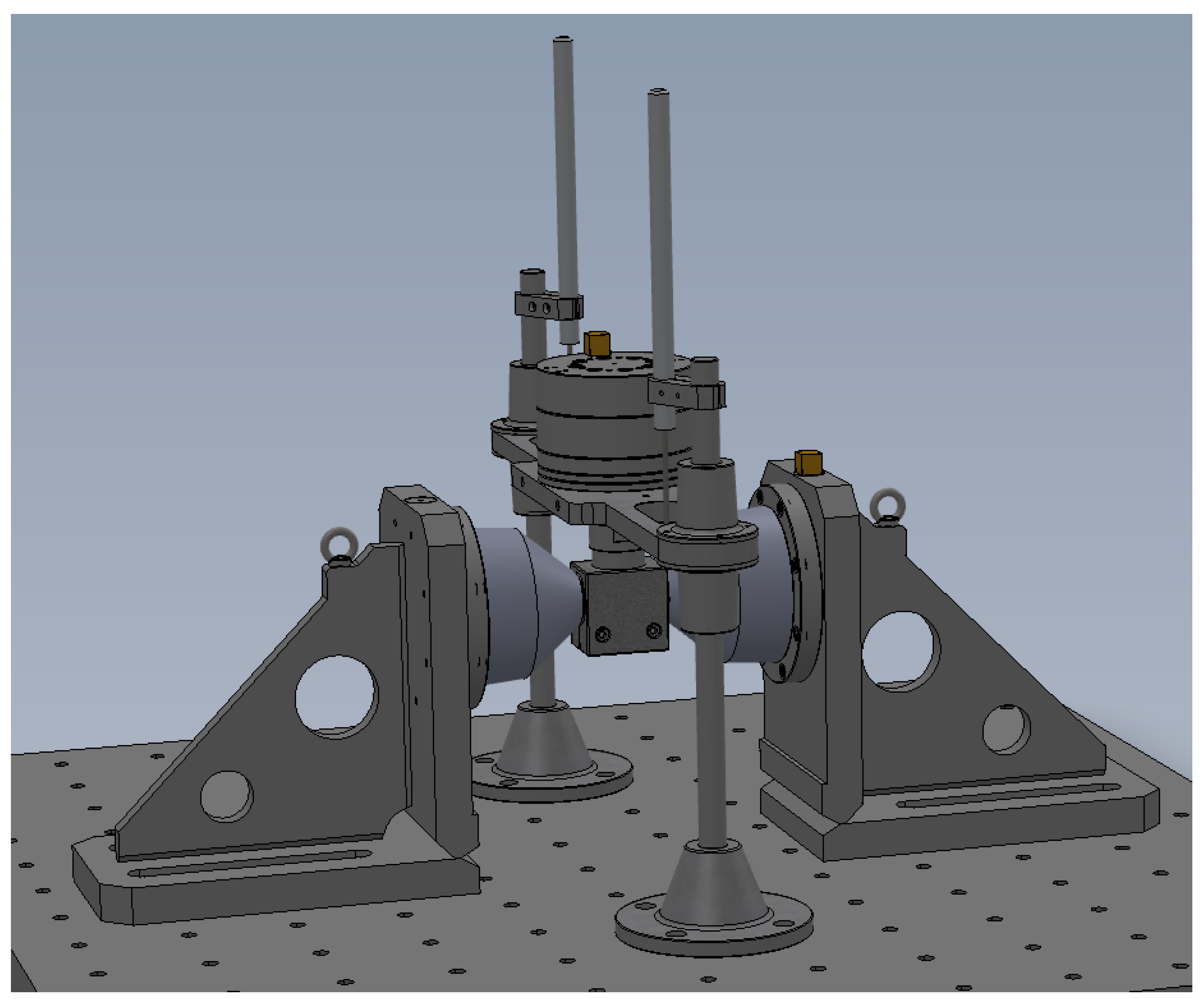
Figure 21.
Picture of elastomer shockmounts in shear configuration.

Figure 22.
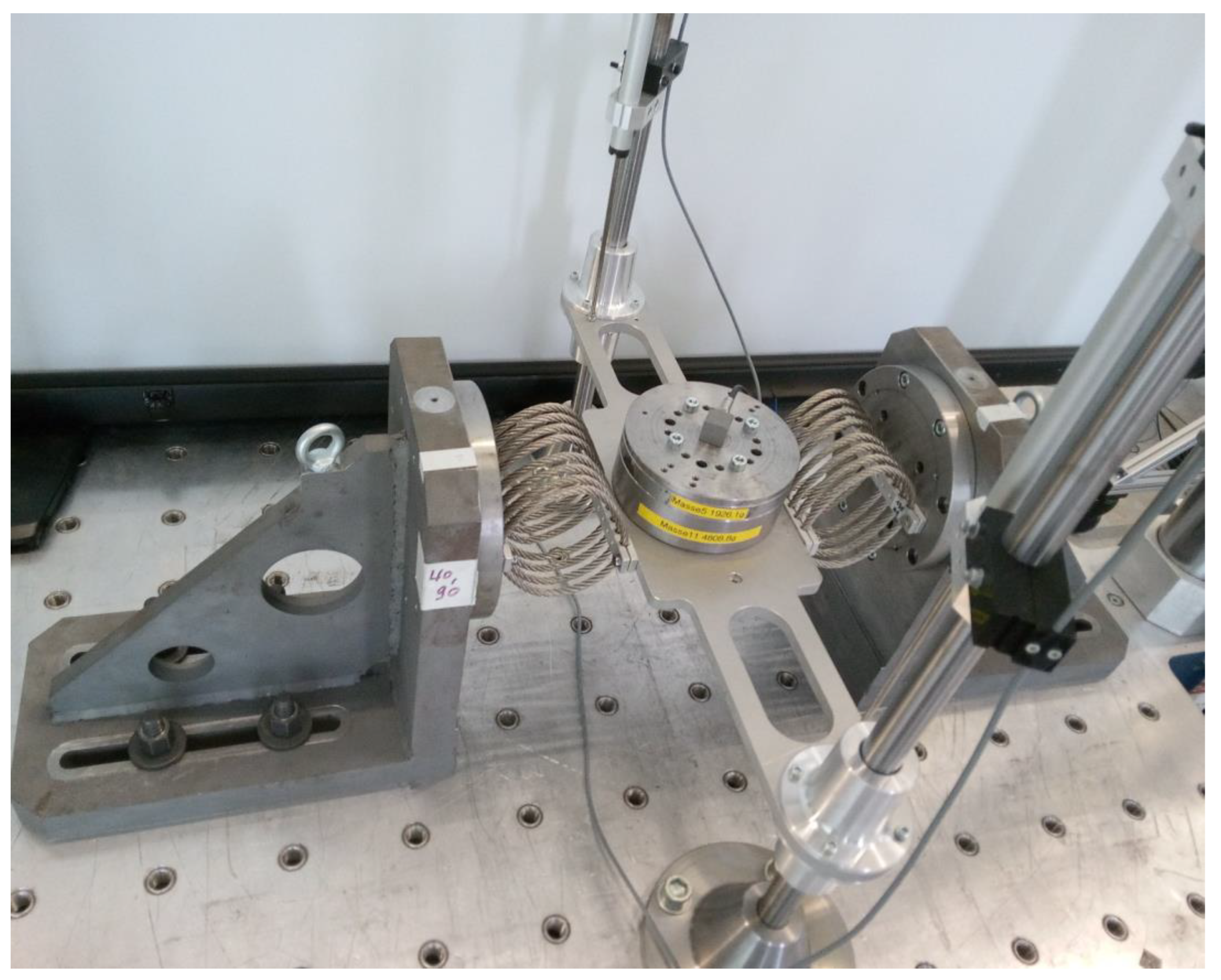
Sketch of wire rope shockmounts in roll configuration.
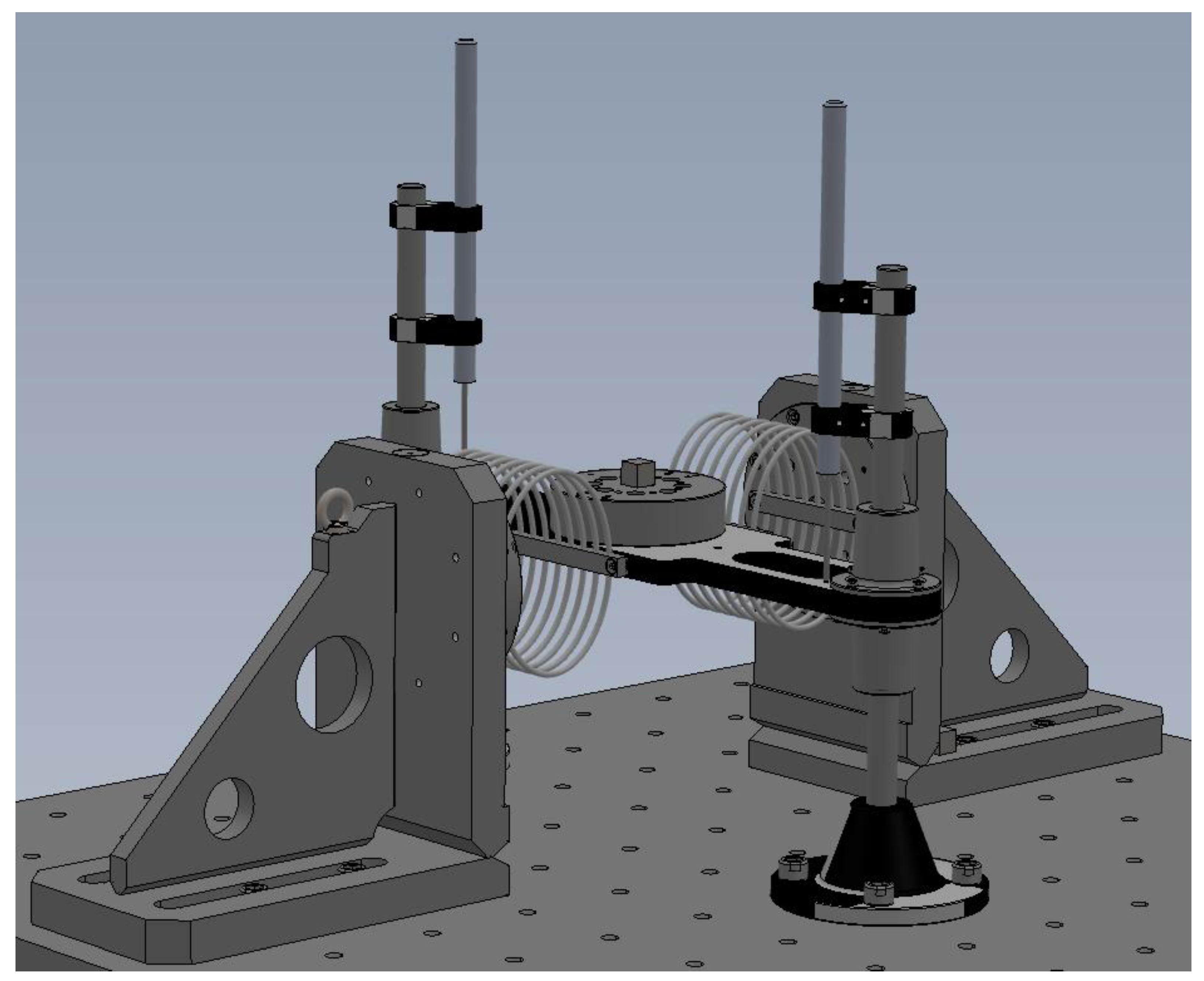
Figure 23.
Picture of wire rope shockmounts in roll configuration.

Figure 24.
Sketch of wire rope shockmounts in shear configuration.

Figure 25.
Picture of wire rope shockmounts in shear configuration.
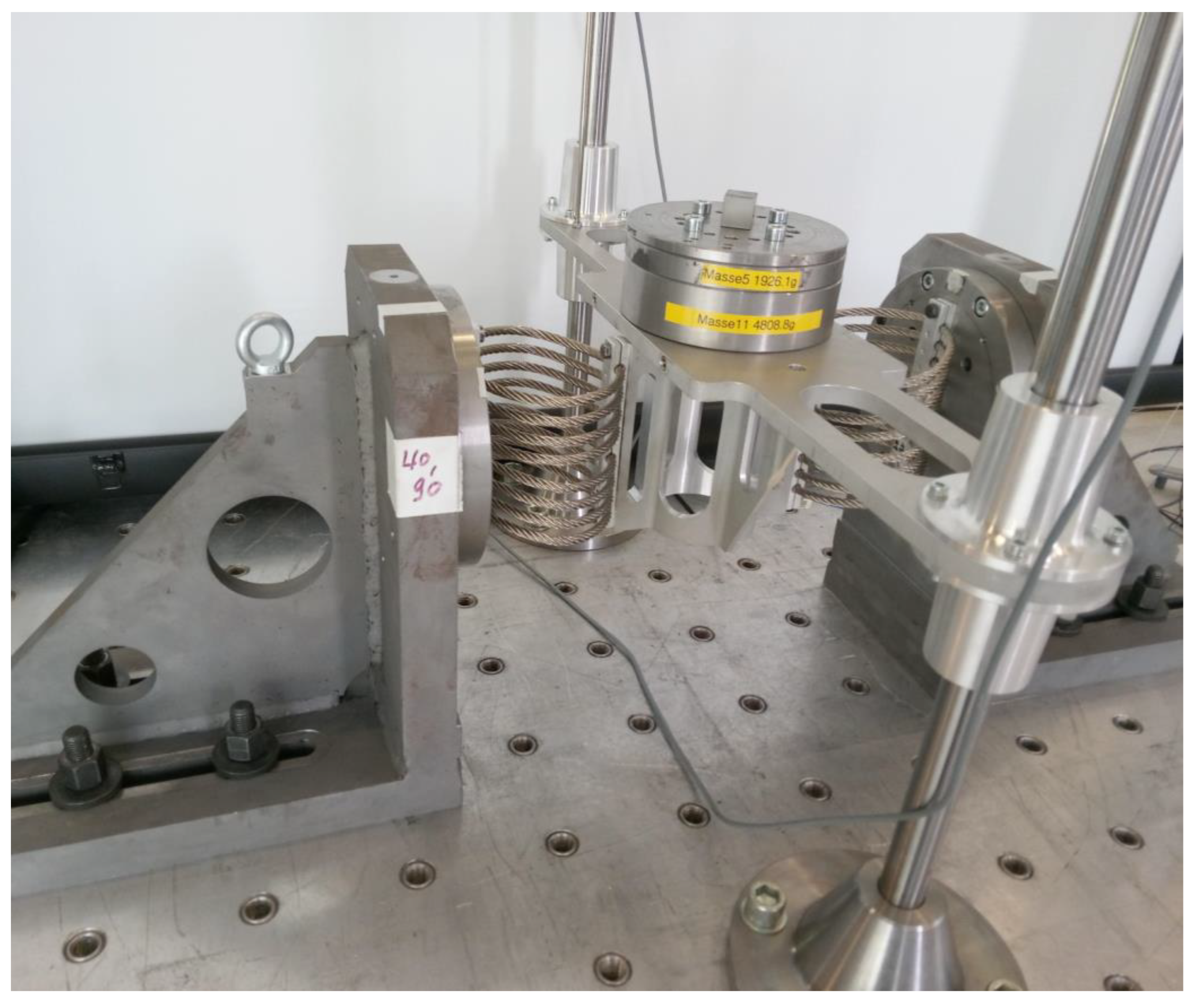
Figure 26.
Highspeed camera with LED spots.
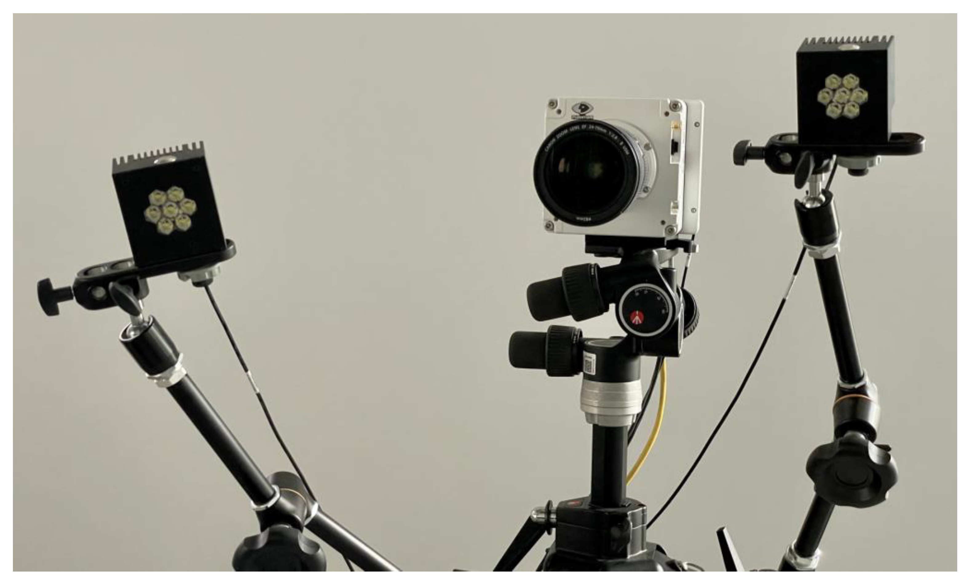
Figure 27.
Acceleration signals.
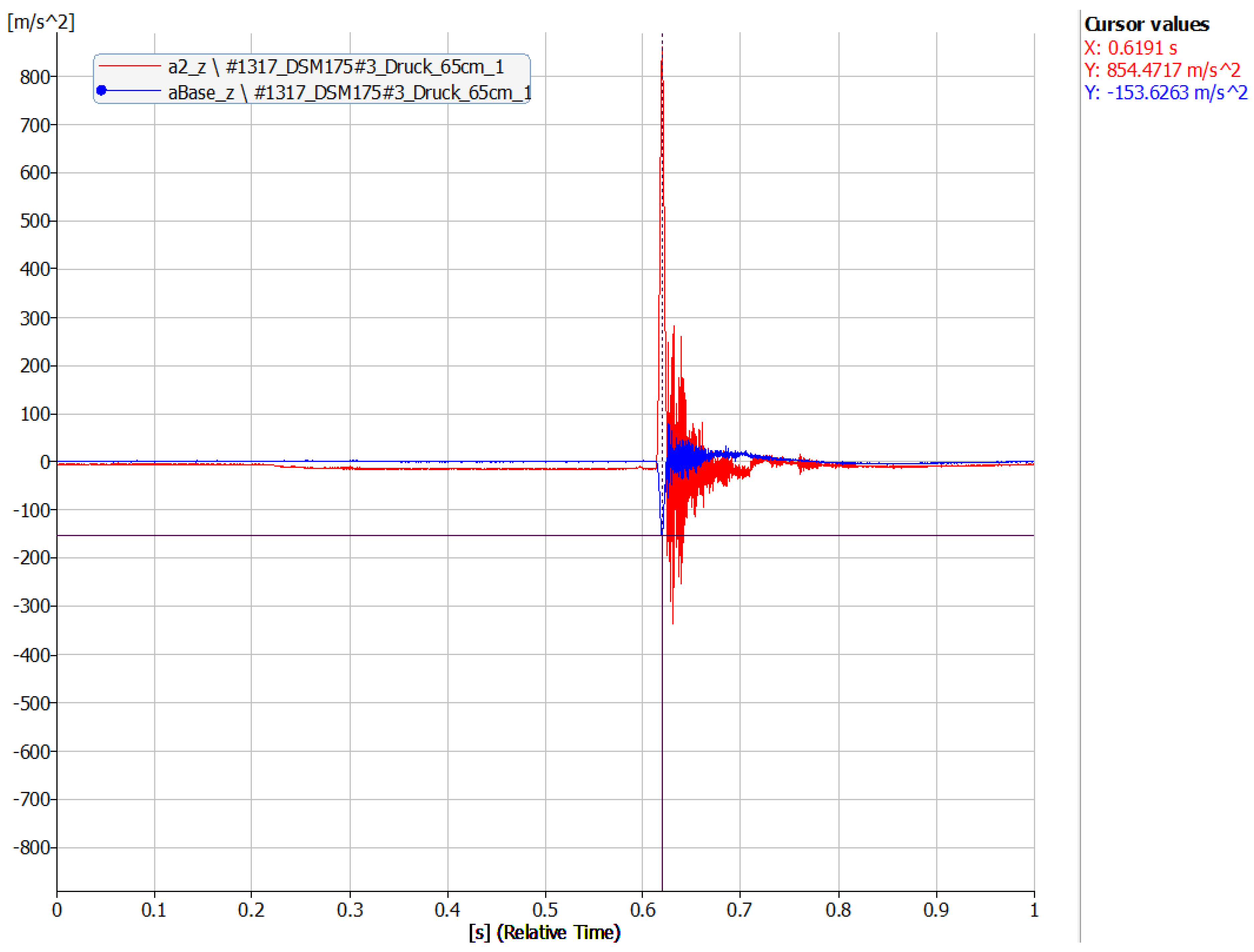
Figure 28.
Closeup of acceleration signals before impact.

Figure 29.
Acceleration signals around impact.
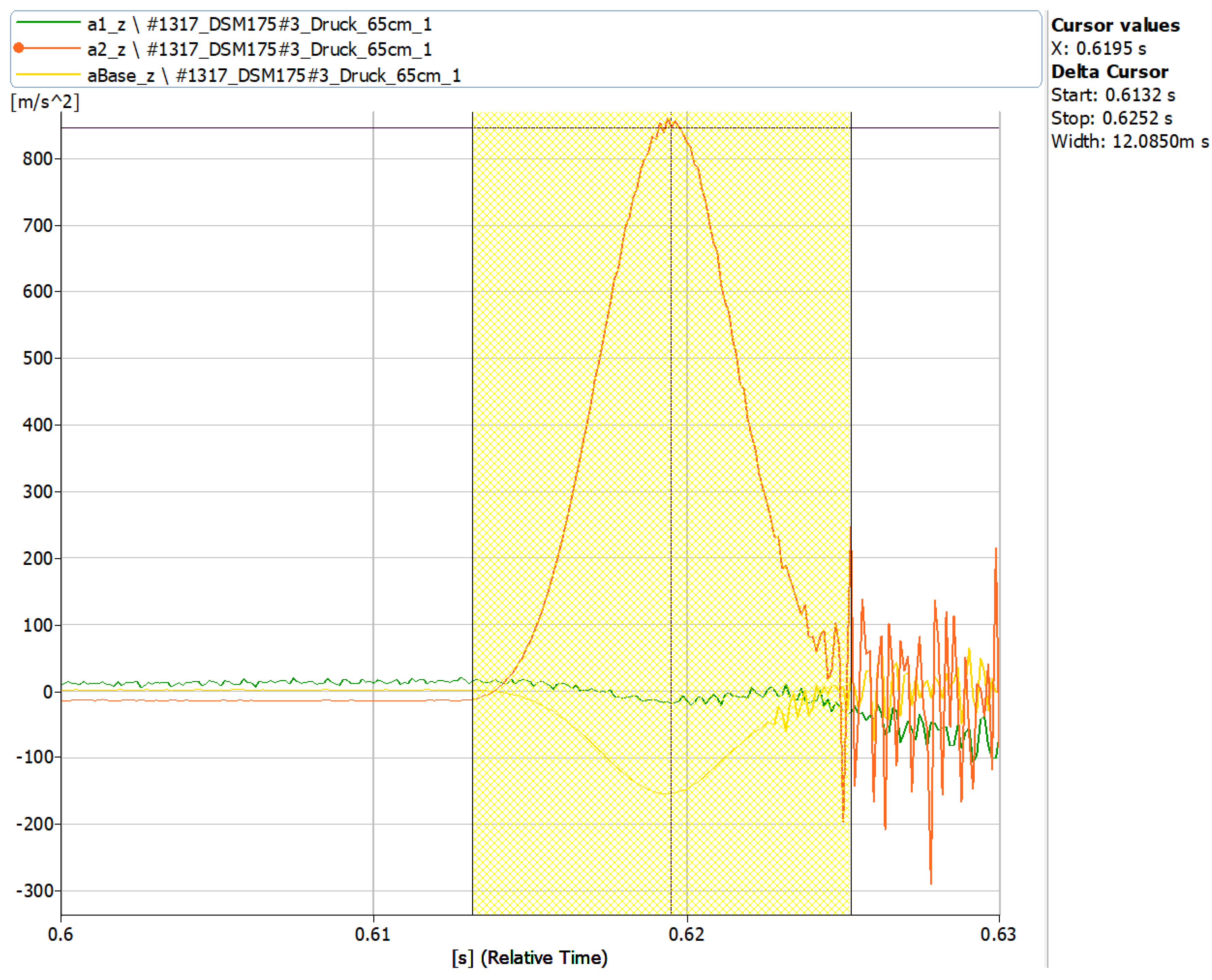
Figure 30.
Acceleration signals during and after impact.
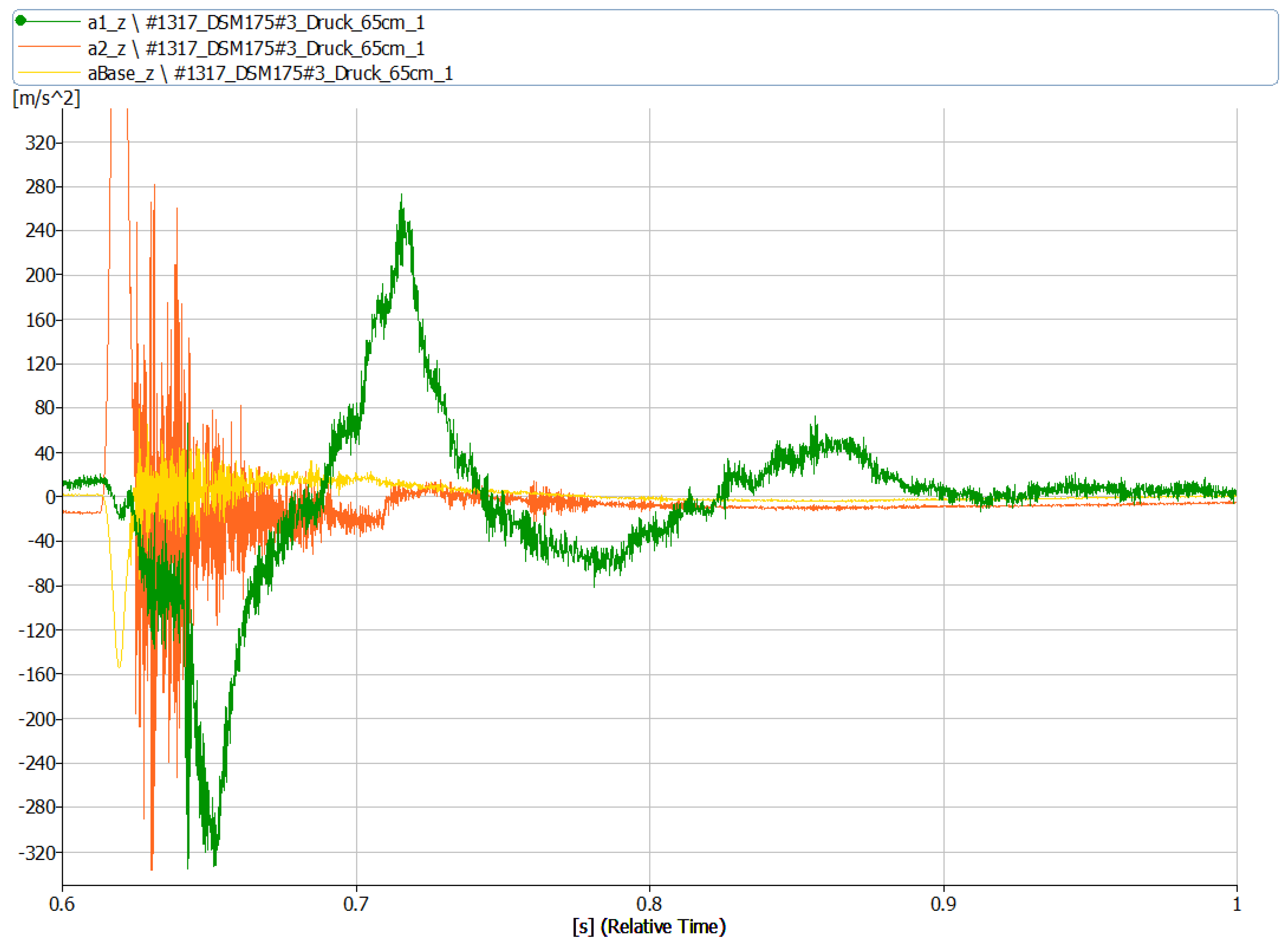
Figure 31.
Acceleration signal, a1_z, and displacement of the shockmount.
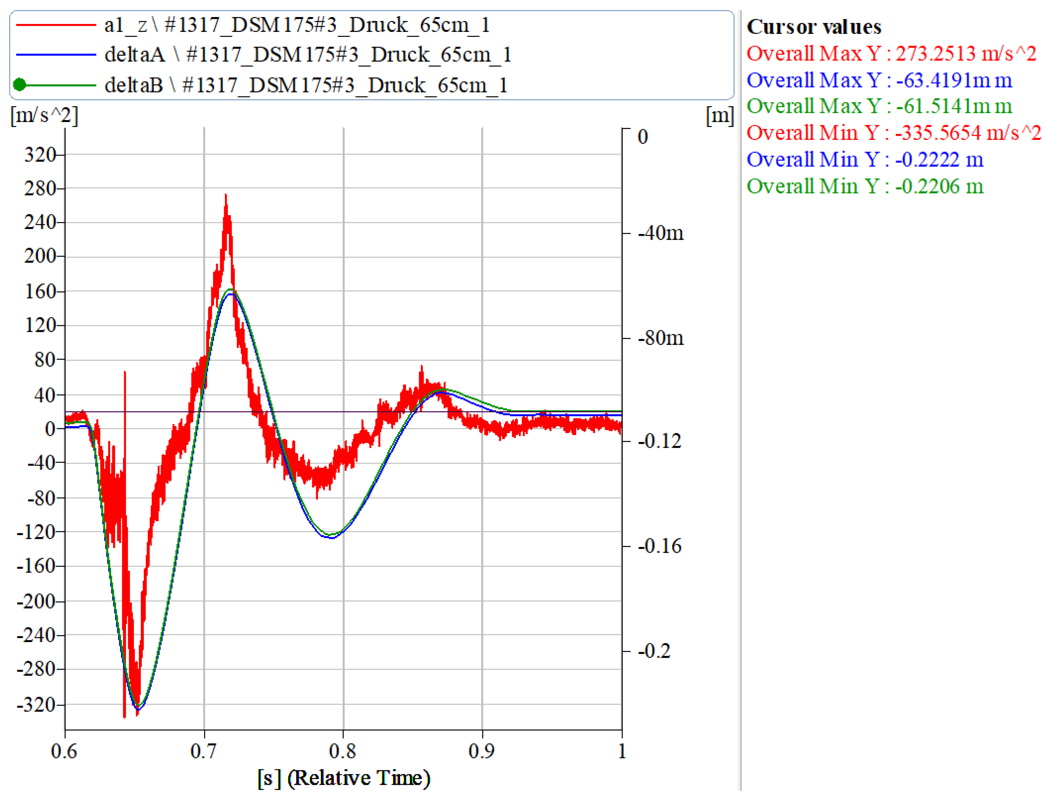
Figure 32.
Acceleration signals of basepoint excitation with 10 runs and fixed parameters.

Figure 33.
Overall maximal acceleration with 10 runs and fixed parameters.
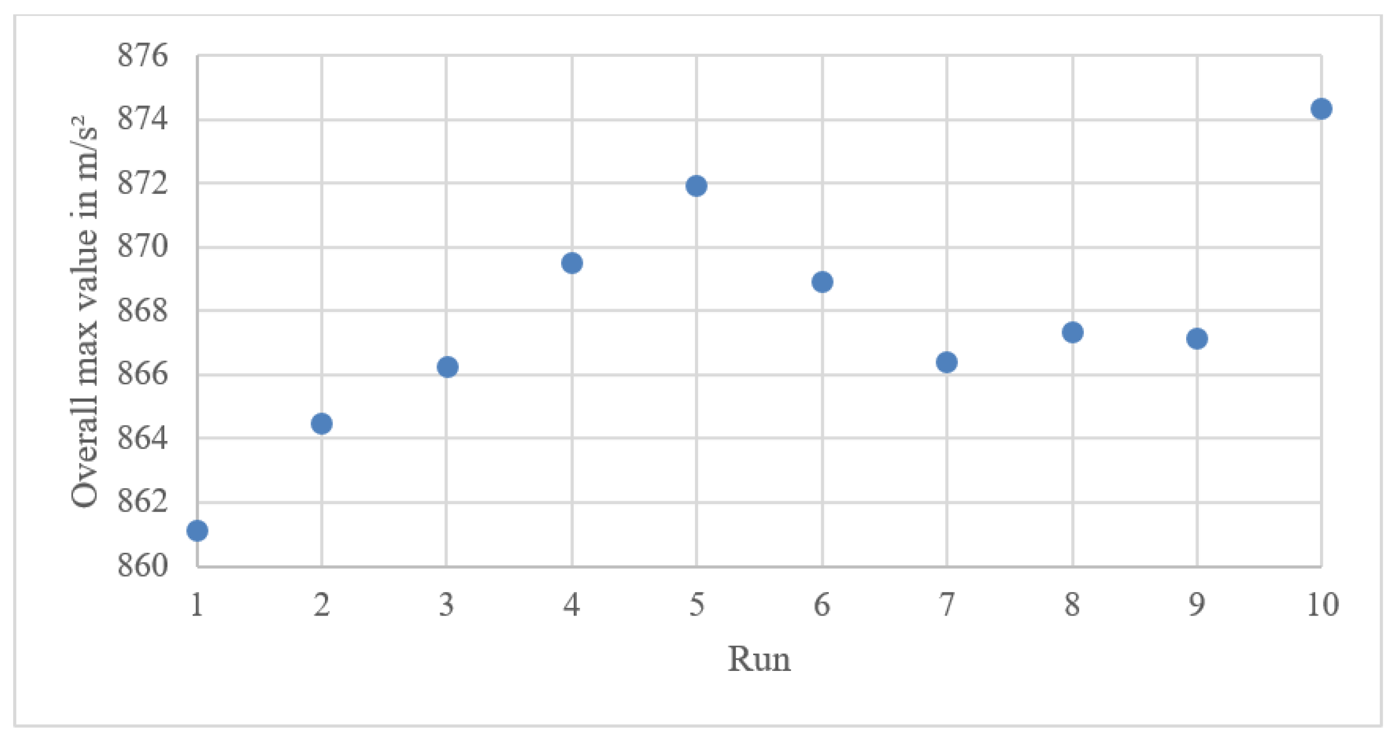
Figure 34.
Exemplary force-displacement diagram of a wire rope shockmount.

Figure 35.
Basepoint acceleration, .

Figure 36.
Simulation programming and solving with ODE45 in MATLAB.
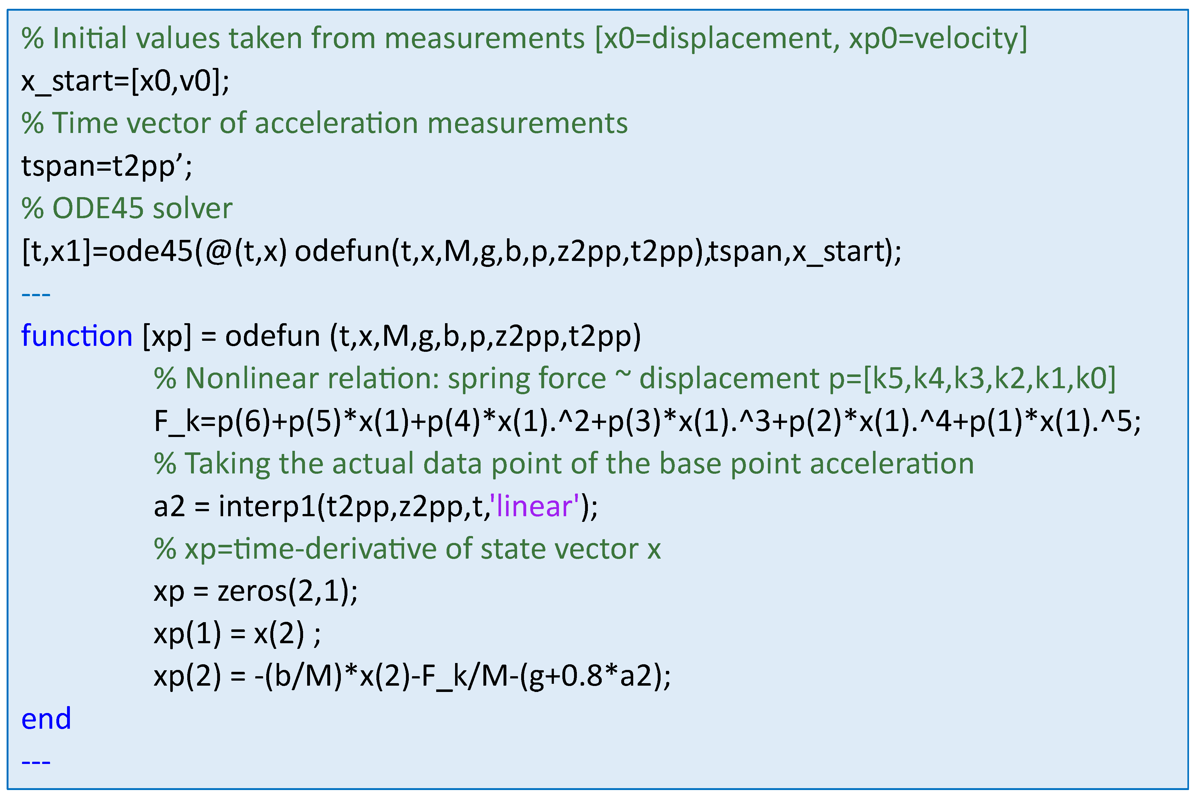
Figure 37.
Simulation and measurement results of the relative displacement time diagram.

Figure 38.
Simulation and measurement results of the relative acceleration time diagram: (a) full measured time range; (b) zoom-in of the haversine impact reaction region.
Figure 38.
Simulation and measurement results of the relative acceleration time diagram: (a) full measured time range; (b) zoom-in of the haversine impact reaction region.
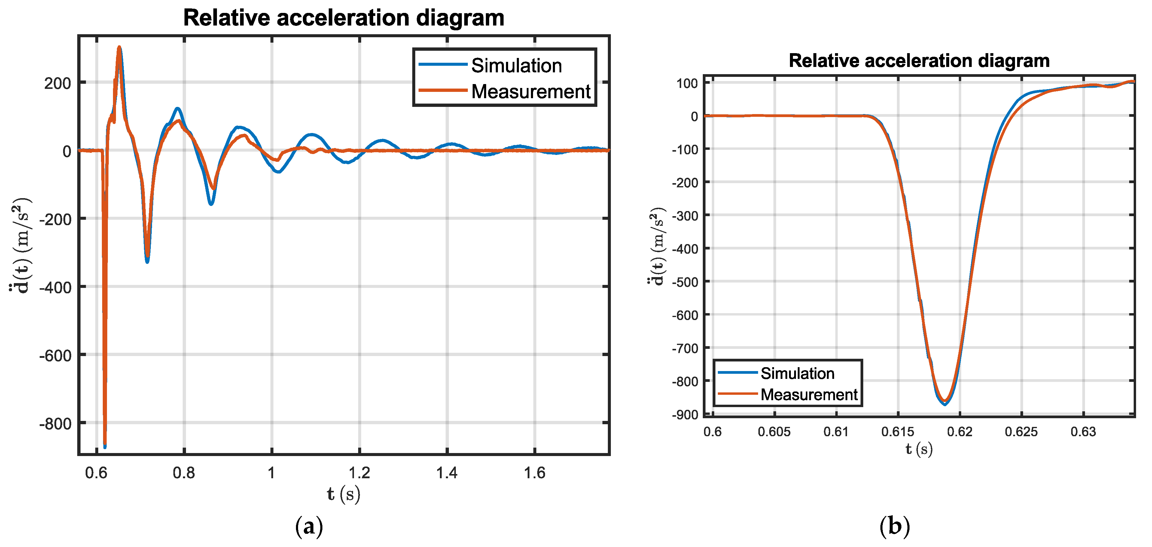
Figure 39.
Simulation and measurement results concerning the first loop of hysteretic behavior of the restoring force.
Figure 39.
Simulation and measurement results concerning the first loop of hysteretic behavior of the restoring force.

Figure 40.
Simulation (a) and measurement (b) results concerning the complete hysteretic behavior of the restoring force.
Figure 40.
Simulation (a) and measurement (b) results concerning the complete hysteretic behavior of the restoring force.
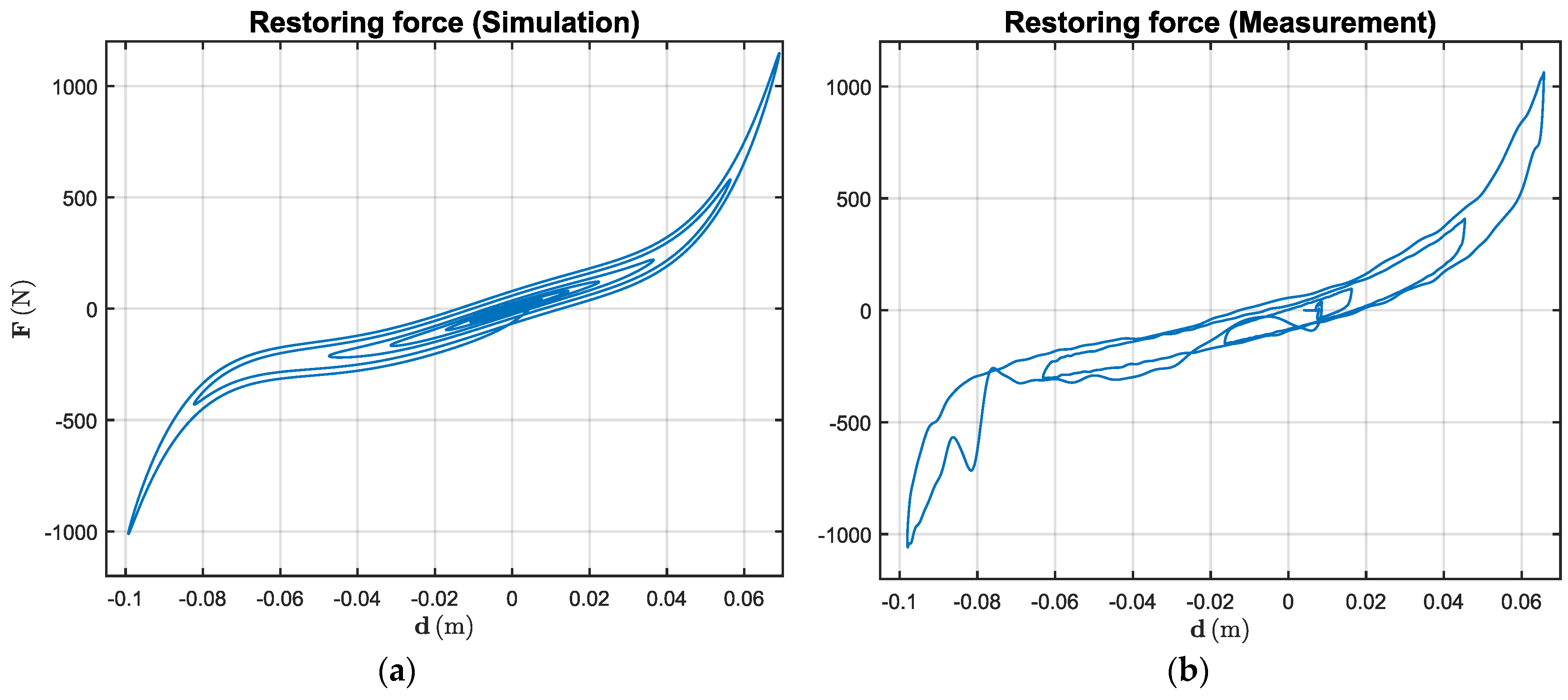
Figure 41.
Simulation and measurement results concerning the nonlinear spring force diagram.


| Type | Manufacturer and Model | Max. Static Load (kg) | Natural Frequency (Hz) @ Max. Static Load | Max. Displacement (mm) in Direction of | |
|---|---|---|---|---|---|
| Tension (+) Compression (−) | Shear, Roll | ||||
| ESM | Willbrandt KG SES 1500 SH32 | 90 | 5 … 6 | 55 | 55 |
| ESM | Willbrandt KG SES 1500 SH40 | 125 | 5 … 6 | 55 | 55 |
| ESM | Willbrandt KG SES 1500 SH55 | 260 | 5 … 6 | 55 | 55 |
| WSM | Willbrandt KG CAVOFLEX H 63-146-135-175-8 | 22 … 120 | 6.2 … 6.7 | +65/−100 | 86 |
| WSM | Willbrandt KG CAVOFLEX H 63-146-110-135-8 | 30 … 150 | 6 … 6.5 | +50/−82 | 65 |
| WSM | Willbrandt KG CAVOFLEX H63-146-95-125-8 | 50 … 170 | 7.1 … 7.6 | +45/−67 | 60 |
Table 2.
Measured signals.
| Signal Name | Sensor Type | Position | Purpose |
|---|---|---|---|
| a1_z | Triaxial MEMS accelerometer | Loading mass | Measuring vertical acceleration of upper part |
| a2_z | Uniaxial MEMS accelerometer | Basepoint | Measuring vertical acceleration of lower part |
| aBase_z | Uniaxial MEMS accelerometer | Seismic base | Measuring vertical acceleration of base |
| deltaA | Linear potentiometer | Between rod and traverse of guide system | Measuring displacement between basepoint and loading mass |
| deltaB | Linear potentiometer | Between rod and traverse of guide system | Measuring displacement between basepoint and loading mass |
Table 3.
Stiffness coefficients of the nonlinear spring force.
| Parameter | ||||||
|---|---|---|---|---|---|---|
| Value | − | − |
Table 4.
Parameters of mass, equivalent stiffness, and damping.
| Parameter | ||||
|---|---|---|---|---|
| Value | 3.449 |
Table 5.
18 exemplary configurations, and their damping and stiffness parameters. H, M, and L stand for high, middle, and low drop height.
Table 5.
18 exemplary configurations, and their damping and stiffness parameters. H, M, and L stand for high, middle, and low drop height.
| Compr. | Tension | Shear | Roll | Damp. | Stiffness from Parameter Identification | ||||||||||||||
|---|---|---|---|---|---|---|---|---|---|---|---|---|---|---|---|---|---|---|---|
| SM | H | M | L | H | M | L | H | M | L | H | M | L | |||||||
| ESM32#1 | X | 2.6 | −2.67 × 10² | 1.34 × 10⁻¹ | −1.60 × 10⁻⁴ | −2.09 × 10⁻⁵ | 7.86 × 10⁻⁸ | 3.66 × 10⁻⁹ | |||||||||||
| #2 | X | 3.2 | −1.07 × 10⁻² | 1.29 × 10⁻¹ | −8.51 × 10⁻⁵ | −1.84 × 10⁻⁵ | 5.22 × 10⁻⁸ | 2.83 × 10⁻⁹ | |||||||||||
| #3 | X | 2.2 | 5.15 × 10⁻³ | 7.76 × 10⁻² | 1.07 × 10⁻⁵ | −8.85 × 10⁻⁶ | −4.94 × 10⁻⁹ | 1.22 × 10⁻⁹ | |||||||||||
| ESM40#1 | X | 2,6 | −4.40 × 10⁻² | 1.47 × 10⁻² | −1.98 × 10⁻⁴ | −2.44 × 10⁻⁵ | 9.96 × 10⁻⁸ | 4.34 × 10⁻⁹ | |||||||||||
| #2 | X | 2.6 | −3.01 × 10⁻² | 1.44 × 10⁻¹ | −1.27 × 10⁻⁴ | −2.16 × 10⁻⁵ | 7.63 × 10⁻⁸ | 3.23 × 10⁻⁹ | |||||||||||
| #3 | X | 2.3 | −8.73 × 10⁻³ | 8.96 × 10⁻² | 6.21 × 10⁻⁶ | −1.01 × 10⁻⁵ | −2.55 × 10⁻⁹ | 1.37 × 10⁻⁹ | |||||||||||
| ESM55#1 | X | 4.2 | −5.85 × 10⁻² | 2.2 × 10⁻¹ | −3.03 × 10⁻⁴ | −5.09 × 10⁻⁵ | 2.08 × 10⁻⁷ | 1.34 × 10⁻⁸ | |||||||||||
| #2 | X | 4.6 | −2.21 × 10⁻² | 2.41 × 10⁻¹ | 5.45 × 10⁻⁵ | −4.74 × 10⁻⁵ | 3.21 × 10⁻⁸ | 1.17 × 10⁻⁸ | |||||||||||
| #3 | X | 4.1 | −1.67 × 10⁻² | 1.37 × 10⁻¹ | 3.18 × 10⁻⁵ | −1.92 × 10⁻⁵ | −2.54 × 10⁻⁸ | 3.77 × 10⁻⁹ | |||||||||||
| WSM125#1 | X | 5.0 | 1.27 × 10⁻² | 1.28 × 10⁻² | 9.97 × 10⁻⁶ | 4.91 × 10⁻⁷ | 1.50 × 10⁻⁷ | 2.44 × 10⁻⁹ | |||||||||||
| #2 | X | 4.3 | 1.23 × 10⁻² | 1.58 × 10⁻² | 3.35 × 10⁻⁵ | −6.05 × 10⁻⁶ | 1.42 × 10⁻⁷ | 6.07 × 10⁻⁹ | |||||||||||
| #3 | X | 9.8 | −5.03 × 10⁻³ | 2.94 × 10⁻³ | 2.81 × 10⁻⁵ | 1.01 × 10⁻⁶ | −5.11 × 10⁻⁸ | 7.55 × 10⁻¹⁰ | |||||||||||
| WSM135#1 | X | 6.9 | 8.92 × 10⁻³ | 1.04 × 10⁻² | 5.99 × 10⁻⁵ | 1.93 × 10⁻⁶ | 8.90 × 10⁻⁸ | 1.03 × 10⁻⁹ | |||||||||||
| #2 | X | 5.0 | −1.11 × 10⁻² | 1.38 × 10⁻² | 2.16 × 10⁻⁴ | −1.14 × 10⁻⁵ | −1.01 × 10⁻⁷ | 8.91 × 10⁻⁹ | |||||||||||
| #3 | X | 9.6 | −2.34 × 10⁻⁴ | 2.52 × 10⁻³ | 5.50 × 10⁻⁶ | 2.80 × 10⁻⁷ | −4.80 × 10⁻⁹ | 1.32 × 10⁻¹⁰ | |||||||||||
| WSM175#1 | X | 6.4 | 9.12 × 10⁻³ | 5.16 × 10⁻³ | 1.18 × 10⁻⁷ | −3.09 × 10⁻⁷ | 2.02 × 10⁻⁸ | 2.84 × 10⁻¹⁰ | |||||||||||
| #2 | X | 5.0 | 3.84 × 10⁻³ | 6.15 × 10⁻³ | −3.78 × 10⁻⁶ | −1.23 × 10⁻⁶ | 2.14 × 10⁻⁸ | 4.90 × 10⁻¹⁰ | |||||||||||
| #3 | X | 11.3 | 3.68 × 10⁻⁴ | 9.26 × 10⁻⁴ | 1.72 × 10⁻⁶ | 1.34 × 10⁻⁷ | −1.70 × 10⁻⁹ | 2.03 × 10⁻¹¹ | |||||||||||
Disclaimer/Publisher’s Note: The statements, opinions and data contained in all publications are solely those of the individual author(s) and contributor(s) and not of MDPI and/or the editor(s). MDPI and/or the editor(s) disclaim responsibility for any injury to people or property resulting from any ideas, methods, instructions or products referred to in the content. |
© 2023 by the authors. Licensee MDPI, Basel, Switzerland. This article is an open access article distributed under the terms and conditions of the Creative Commons Attribution (CC BY) license (https://creativecommons.org/licenses/by/4.0/).
Share and Cite
MDPI and ACS Style
Heinemann, B.; Simanowski, K.; Clasen, M.; Dreesen, J.; Sachau, D. A Testbench for Measuring the Dynamic Force-Displacement Characteristics of Shockmounts. Vibration 2024, 7, 1-35. https://doi.org/10.3390/vibration7010001
AMA Style
Heinemann B, Simanowski K, Clasen M, Dreesen J, Sachau D. A Testbench for Measuring the Dynamic Force-Displacement Characteristics of Shockmounts. Vibration. 2024; 7(1):1-35. https://doi.org/10.3390/vibration7010001
Chicago/Turabian StyleHeinemann, Bernhard, Kai Simanowski, Michael Clasen, Jan Dreesen, and Delf Sachau. 2024. "A Testbench for Measuring the Dynamic Force-Displacement Characteristics of Shockmounts" Vibration 7, no. 1: 1-35. https://doi.org/10.3390/vibration7010001