

A Nonparametric Regularization for Spectrum Estimation of Time-Varying Output-Only Measurements

1
Department of Engineering Technology, Vrije Universiteit Brussel, Pleinlaan 2, 1050 Brussels, Belgium
2
Brussels Institute for Thermal-Fluid Systems and Clean Energy (BRITE), Vrije Universiteit Brussel (VUB) and Université Libre de Bruxelles (ULB), 1050 Brussels, Belgium
*
Author to whom correspondence should be addressed.
Vibration 2024, 7(1), 161-176; https://doi.org/10.3390/vibration7010009
Submission received: 17 November 2023
/
Revised: 26 January 2024
/
Accepted: 7 February 2024
/
Published: 7 February 2024
Abstract
:In this work, an advanced 2D nonparametric correlogram method is presented to cope with output-only measurements of linear (slow) time-varying systems. The proposed method is a novel generalization of the kernel function-based regularization techniques that have been developed for estimating linear time-invariant impulse response functions. In the proposed system identification technique, an estimation method is provided that can estimate the time-varying auto- and cross-correlation function and indirectly, the time-varying auto- and cross-correlation power spectrum estimates based on real-life measurements without measuring the perturbation signals. The (slow) time-varying behavior means that the dynamic of the system changes as a function of time. In this work, a tailored regularization cost function is considered to impose assumptions such as smoothness and stability on the 2D auto- and cross-correlation function resulting in robust and uniquely determined estimates. The proposed method is validated on two examples: a simulation to check the numerical correctness of the method, and a flutter test measurement of a scaled airplane model to illustrate the power of the method on a real-life challenging problem.
1. Introduction
The paper presents a nonparametric estimation technique for output-only measurements of time-varying mechanical and civil structures. These types of measurements are the so-called operational measurements [1]. These measurements are crucial because it is common that systems tend to exhibit different dynamical behavior when observed under operating conditions than observed under laboratory conditions. To explore the behavior in operating conditions is important because unobserved and unmodeled phenomena may lead to structural failures or unstable operation.
Operational measurements proved to be successful in civil engineering, where it is difficult to obtain artificially induced vibration levels that exceed the natural vibrations due to traffic or wind [2,3,4]. It is also a popular approach in various mechanical engineering applications; think of, for instance, the road testing of a vehicle [5,6,7]. These types of measurements are commonly used in aerodynamics; for instance, studying vortex-induced vibration [8,9].
The main challenge with the Operational Modal Analysis (OMA) framework—in comparison with the classical identification frameworks—is that the perturbation (excitation) is not (or cannot be) measured directly, and instead it is assumed to be (nearly) white noise around the frequency domain of interest [1]. Methods for OMA have hence been developed and are now widely used in the industrial environment [2]. This can be used (1) to better understand the true underlying system [1], (2) to simulate the system [10], and (3) to validate and update computer-based models such as finite element models, for instance [11,12].
In the case of nonparametric OMA (or in general, output-only measurements), the most common goal is to estimate the output power spectral density function (PSD). Given a (time domain) measurement, the auto-power spectrum can be estimated via different techniques; for an exhaustive list of OMA techniques, we refer to [13].
The most commonly used nonparametric methods are the (time domain) correlogram- and the (frequency domain) periodogram-based procedures [14,15]. In the case of correlogram techniques, different types of output autocorrelation functions (ACF) are estimated, then transformed to the (discrete) frequency domain resulting in a PSD estimate [16]. Because the raw ACF-based time estimate may result in a non-smooth estimate of the power spectrum (i.e., the estimate has high variance level), therefore, additional windowing (typically exponential windowing) is usually applied [1] to overcome this issue. The drawback is that the damping factor will be overestimated, due to the windowing applied to the time domain signal. The user must manually decide on the type of window function and its parameters (e.g., the decaying rate of the exponential window).
In the case of a simple periodogram (squared discrete Fourier transform of the measured signal), the variance issues are even more pronounced. There are two popular possibilities to reduce the variance of the periodogram estimate. One of the possibilities is to use averaging techniques such as Bartlett’s method, where the estimate is calculated on the (special) averaged periodograms of the segmented measurement [17]. The drawback is that this method results in a decreased frequency resolution of the estimate. Welch’s method is another popular possibility where the data segments are overlapped, and an additional windowing function is applied [18]. In the latter case, the variance of the PSD estimate is decreased, and the bias error is significantly increased (resulting in an overestimating of the damping factor).
The state-of-the-art STFT implementations include, among others, efficient methods for time-of-flight problems [19], identification of wireless devices [20], and modeling of electric energy losses [21]. Ref. [22] proposes a combination of STFT and a convolutional neural network to postprocess 1D ECG signals into 2D spectrograms.
In this paper we consider generic linear time-varying (LTV) systems. The dynamical properties of such systems (such as damping ratios, resonance frequencies) may vary significantly when operating conditions (such as wind speed, pitch angle, temperature, mass, etc.) change. Ignoring these variations might lead to poor product quality, instability, and structural failures. Therefore, it is crucial to use OMA models that can capture time variations. It is a common practice in system identification and in modal analysis to use different types of short-time Fourier transform (STFT) methods that are suitable to cope with (very) slow time-variations. The idea of these techniques is to create a series of linear-time invariant (LTI) models [23,24] which make use of the above-mentioned simple to implement techniques. These STFT-based models can describe the time-varying behavior quite well, when the time-variations are very smooth (i.e., the system varies very slowly). Therefore, these models cannot cope with fast(er) or sudden variations.
In this work, we provide a novel 2D TV kernel function-based regularization technique to overcome the issues of the classical STFT-based methods, thus allowing more accurate modeling in cases of faster time-variations. The kernel-based methods are a quasi-extension of the well-known Tikhonov regularization techniques [25,26]. In the classical regularization methods, impulse response estimates of LTI systems are considered [27,28]. There are technically more-involved hybrid nonparametric and parametric regularization-based methods that are applied for time-invariant dynamic networked system identification problems [29,30,31]. It is important to mention that none of the already existing techniques cope with output-only problems.
The main novelty of this work is that the nonparametric regularization is applied to output-only measurements of LTV. The proposed robust 2D regularization techniques make the uniquely determined TV auto- and cross-correlation function possible. By robustness we mean the system identification concept: the estimation framework applied in this work results in reliable and statistically correct estimates in the presence of noise and outliers. The proposed method is illustrated on a simulation example with (a high level of) noise, and on a real-life flutter test measurement of a scaled airplane—containing both noise and outliers.
This paper is structured as follows. In Section 2, the basic definitions, concepts, and assumptions of this work are summarized. Section 3 provides the model structure and the cost function of the underlying problem and summarizes the practical considerations of the proposed technique. Section 4 and Section 5 show a simulation and a measurement example. Finally, conclusions are provided in Section 6.
2. Basics
2.1. Considered Systems and Assumptions
Assumption 1.
The time-domain (discrete) output response of a time-varying system to an arbitrary time domain signal at time instance is nonparametrically given by [33,34]:
where is the time-varying impulse response function (also known as 2D impulse response function), the parameter is the measurement time (the time instance when the system is observed [35]), is the system time (that represent the lags of the impulse response coefficients), and is the convolution operator.
An LTV system represented by is causal when the following is true:
When a finite observation (measurement) with samples is considered, with an impulse response length , then (1) boils down:
To make the text more accessible, the time indices will be omitted. The LTV system represented by is linear when the superposition principle is satisfied:
where and are scalar values.
Because time-varying systems are often misinterpreted as nonlinear systems, it is important to mention that when varies with and (and the variation depends also on the excitation signal ), then the system is called nonlinear [36,37].
Assumption 2.
The considered systems are smooth: the finite differences between the adjacent points of in both time directions () are relatively small. A detailed study on smoothness can be found in [38].
Assumption 3.
For the estimators to work is needed: the measurement must be longer than the impulse response function.
Assumption 4.
The measurement has a constant sampling time. The output is measured with additive, i.i.d. Gaussian noise (denoted by in the time-domain) with zero mean and finite variance , such that the measurement is given by:
Assumption 5.
The exact excitation signal is unknown but is assumed to be (nearly) white (in the frequency band of interest) with a finite variance of .
2.2. Non-Uniqueness Issues
The challenge in nonparametric system identification is that cannot be uniquely determined from a single set of measurements. This means that consists of parameters that cannot be directly determined using measurement samples. An illustration can be seen in Figure 1, where the true system is estimated by the means of Maximum Likelihood (ML) estimators: observe that the result does not resemble the original model. The application of Assumptions 1–4 allows us to have uniquely determined (smooth and decaying) solutions in case of known input for , or for the TV autocorrelation function in case of unknown input when Assumption 5 is also fulfilled. This can be achieved by using smoothing methods, for instance: spline interpolation or nonparametric kernel-based regularization.
3. The Proposed Identification Method
3.1. The Model
In the case of OMA measurements, the frequency response function (FRF) model cannot be directly estimated. However, output only data allows us to estimate the power spectrum estimates—similarly to FRF estimates. When the Assumptions 1–5 are fulfilled, the underlying systems can be uniquely estimated by their ‘scaled’ 2D TV FRFs. The scaling in this case means that the exact level of excitation is unknown, but due to the whiteness assumption of the perturbation, the estimated power spectrum corresponds to the FRF but scaled by an unknown factor. This process is illustrated in Figure 2.
In this work, a novel nonparametric method is provided to identify the time-varying auto-correlation function of output-only measurements. To keep the complexity under control, the proposed technique is illustrated with a single output, but it can be generalized to measurements with multiple outputs. The advantage of using multiple outputs (sensors) is that the phase relationship between different (sensory) locations can be obtained. In this case not only the magnitude values of the ‘scaled’ 2D TV FRFs can be obtained, but also an estimation of the phase values. These estimated phase values may play an important role when the end-users are interested in estimating the operational deflection shapes.
When Assumptions 1–5 are fulfilled, the time-varying auto-correlation function boils down to a modified auto-correlation function centered around as follows:
Note that depending upon the application area, different weightings of (6) are possible: for more details see [15].
3.2. The Cost Function
In this output-only framework, the ML cost function of the time-varying autocorrelation estimate boils down to LS (least square) cost function that is given by:
where vect(X) stands for the column-wise vectorization of X, is the measured LTV autocorrelation obtained using (6), and is the true LTV model. It is important to emphasize that the ML cost function will only be simplified to the LS cost function when the assumptions on the measurement noise are fulfilled. If this assumption (Assumption 4) is not (entirely) fulfilled, then this will result in an additional (bias) error because when modeling colored noise, more complex modeling structures are needed. For a further elaboration we refer to [32,39].
The key idea of the regularization technique is to keep the model complexity under control in a way that any deviation from the assumptions is punished. This will introduce on the cost level some small bias error to the classical LS cost function that results in a lower variance that ultimately results in a lower total (mean square) error [40]. The new combined regularized cost function is given by:
where is the (regularization) covariance matrix that contains the assumptions (a prior knowledge), and is the amount of regularization applied that corresponds to the variance (estimate) of the output measurement ().
Evaluating the cost function (8) can be completed by solving the equation as shown in the following main steps—for the sake of simplicity from here on vect() will be omitted:
that results in the following estimate:
where is the identity matrix.
To illustrate the concept of the regularization, an LTI example is shown in Figure 3. The classical LS solution of the auto-correlation estimate oscillates in the tail part that results in high variance (manifested as leakage) in the frequency domain. In the regularized least squares (RLS) case, smoothness and stability is imposed such that the tail decays toward zero. The fitting error of the regularized PSD estimate in this case results in approximately two times lower error.
3.3. The Kernel Functions
The covariance matrix encodes assumptions about the system and it is obtained using the so-called kernel functions. This is implemented in this work as a special correlation between the elements of the 2D ACF. The specific choice of these kernel functions will have a major impact on the estimation quality. Next, the kernels that are considered in this framework will be briefly elaborated. A graphical illustration of the proposed kernel function on an impulse response estimation problem is shown in Figure 4.
The RBF (Radial Basis Functions) can impose smoothness between two points as follows [28]:
where . controls smoothness: the higher its value, the smoother the estimate.
To impose exponential decay and smoothness DC (Diagonal Correlated) kernel function can be used [27]:
where controls the smoothness between the autocorrelation coefficients (by imposing higher correlation) and scales the exponential decaying (the shortness of the autocorrelation), . It is possible to reduce the computational needs (at a loss of some flexibility) by setting to . This type of kernel is called TC (tuned correlated) kernel.
3.4. Construction of the Covariance Matrix
Figure 5 shows a TV ACF that correspond to the LTV system illustrated in Figure 1. By analyzing this figure, several properties can be observed. These properties correspond to the assumptions given in Section 2. The goal is to incorporate these properties/encode these assumptions into the covariance matrix .
First, observe that the TV autocorrelation function is smooth in both system time (direction of lags) direction and measurement time direction.
Second, in the system time direction exponential decaying can be observed. This corresponds to the stricter definition of stability: the impulse responses and hence the auto- and cross-correlation functions are exponentially decaying. This decaying behavior is valid for the vast majority of stable vibro-acoustic systems.
From the implementation point of view, the above-mentioned relationships have to be coded in such a way that every point of the 2D ACF is connected to every point. For a measurement with samples and ACF length of , there will be times connections. These connections in fact are constraints that will achieve a unique solution of the rank-deficient estimation problem discussed in Section 2.2.
The TV covariance matrix is then formulated—with DC kernels—as follows:
for every possible pair of and .
3.5. Tuning of the Model Complexity
The proposed nonparametric identification consists of two interrelated steps: (1) optimization of the hyperparameters, and (2) computation of the ACF TV model using (9). , parameters in (9)–(12) are the so-called hyperparameters. These hyperparameters can be optimized, for instance, by maximizing the marginal likelihood function of the observed output [41]:
where is a vector containing all the hyperparameters.
It is important to note that the above-mentioned marginal likelihood function is only valid when the assumption about the measurement noise is fulfilled. This objective Function (14) is non-convex in and therefore, it is advised that the end-users try multiple initializations. For theoretical aspects of the possible optimization techniques, we refer to [38,42].
3.6. Computational Concerns
The computational complexity of the proposed technique is that is quadratically increasing with the number of measured samples (), and with the length of the auto-correlation function ().
The main time-consuming part can be found in the matrix inversion in (9) and in (14). This inversion is performed multiple times during the estimation process. Considering the matrix sizes, it can be clearly seen that by increasing the length of the measurement, the requested operational memory grows quadratically. To reduce the computational complexity, the inversion can be completed using the following matrix equality [40]:
Let us re-order (9) as follows:
Hence, the inversion problem boils down to ) instead of ).
To further simplify the tuning process, it is possible to fix the value of to the estimated variance of the measurement (i.e., ) or using TC kernels instead of DC kernels.
For completeness we like to mention that there exists a filter-based regularization method [43] that in many scenarios results in much lower computational complexity compared to kernel-based methods. However, the LTV reformulation of the filter-based approach is much more involved and therefore it is beyond the scope of this paper.
3.7. Processing Long Measurements
The above-mentioned resource-saving techniques can still be inadequate when working with large datasets. To that end, a sliding window method is proposed. Instead of estimating the computationally demanding TV ACF model in one step, a sliding window technique can be applied to speed up the calculation, and to reduce the memory needs. The technique is illustrated in Figure 6. The 2D regularization technique can be applied within this sliding window that contains only a portion of the large dataset ( samples). After computing the estimates for a set of measurements, the window can be moved with samples. To ensure that the estimates are continuous and overlap , may be needed. At the overlap (see in gray in Figure 6) additional (and optional) RBF smoothing can be applied. If there is overlap, then the effective step size is This means that at each iteration of new ACFs are estimated.
The proposed minimal width of the sliding window () is that is already adequate to provide high quality estimates. Note that mathematically speaking, minimum samples are needed. The step size of the sliding window () should be at least 1. The maximum width is limited to the available memory, but it is advised to use a shorter window in order to speed up the calculations.
The memory need of the proposed sliding window technique is ) instead of the classical ). The computational complexity given by (9) further simplifies to from .
3.8. Guide for Users
In this subsection a user-oriented guide is given. The recommended workflow is shown in Figure 7.
The first step considers the preprocessing of the data where the classical processing steps such as data segmentation, transient removal, and outlier analysis [44] are considered. Using frequency-domain processing it is also possible to have an initial estimate for the measurement noise estimate () [45]. An illustration is shown in Section 4.1.
When multiple output channels (sensors) are available, it is highly recommended to use the most dominant sensor (where the most energy is present or the classical PSD estimate looks the cleanest with highest magnitude values) as a reference sensor. In this case, the first argument of the proposed method—i.e., the first in (6) is the reference channel—and the second channel can be varied—i.e., the second in (6) is the reference channel.
Next, the classical ACF function is recommended to be estimated using all available data (and in the case of multiple channels using the reference channel only). By analyzing the (effective) length of the ACF, a good initial estimate can be obtained for . If needed, one might draw an imaginary exponential envelope around the ACF to determine the length of the ACF. The tail (noisy) part of the ACF (after the imaginary decaying envelop) can be used to provide a weak estimate of the measurement noise (). An illustration is shown in Section 4.1.
Keep in mind that by using spectral analysis the measurement noise can be estimated more accurately. The obtained values of and can be used as fixed hyperparameters. For a first attempt, we recommend starting with TC kernels that have lower computational complexity with usually adequate results. In case of multiple outputs, it is recommended to use the reference channel only, and apply the obtained hyperparameters to other channels without optimizing again.
If there is not enough memory (or the computational complexity seems to be high), then it is recommended to run a sliding window technique instead of the classical “all at once” technique using the processing window (see Section 3.7). We advise to use a step size ( of 15 for a smooth transition overlap () of 5. These settings are believed to be adequate for almost all considered LTV problems.
After running the hyperparameter optimization routine, the obtained results have to be inspected. If the obtained results are inadequate for the intended target application, then first the frequency resolution must be checked. If the frequency resolution turns out to be insufficient for the intended target application, then the value of can be increased. If the frequency resolution seems to be sufficient then one might consider using more regularization (i.e., increase the value of )—especially if the obtained results look too noisy. If the results seem not to be noisy but some details remain hidden, then it is recommended to change the kernel function (for instance to DC kernels).
4. A Simulation Example
4.1. The Model
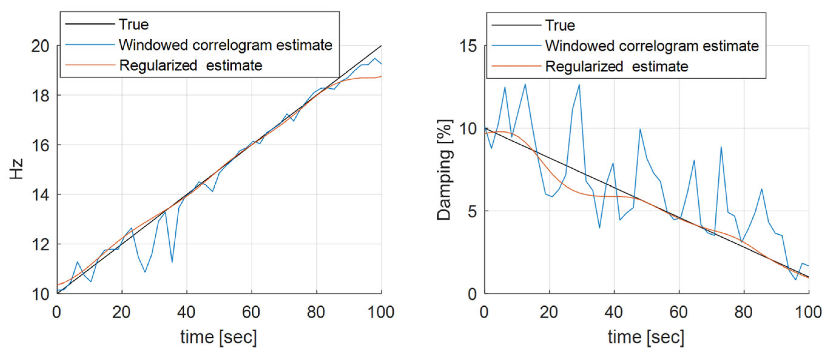
This section presents a simulation example of a second order LTV system. The simulation time is 100 . The damping ratio of the system varies linearly between 10% (at 0 s) and 1% (at 100 s). The resonance frequency (undamped natural frequency) varies between 10 (at 0 s) and 20 Hz (at 100 s). The excitation signal is band-limited white noise (with ), and the output is simulated with an SNR of 20 dB (i.e., . The simulated output signal is discretized with a sampling frequency of 128 that results in a simulation of = 128,000 samples. The system used for the performance test is already shown in Figure 1. It is given by its TV transfer function [39] as follows:
The simulation and the illustration of the proposed estimation method (that is described in Section 3.8) for and are shown in Figure 8. The longest considered ACF contains 12 samples—that is in complete agreement with the ideal impulse response length. To compute the problem at once, the required memory need using 32-bit precision is approximately This means that the sliding window technique should be used. In case of , the required memory need boils down to For the sliding window technique the overlap ) is set to 5.
4.2. The Results
In this section, the parametric estimates of the resonance frequencies and damping ratios are compared, see Figure 9. The results of the traditional STFT approach (windowed correlogram estimates) [23] are compared to the results of the proposed 2D regularization method. In the case of STFT, the output measurement is split into short sub records, and each time the output ACF is calculated, and an additional exponential windowing is applied. This results in a series of ACFs, which represent the classical TV ACF estimate. The power spectrum estimates are provided by the discrete Fourier transform of the ACFs. The resonance frequencies and damping ratios are estimated and tracked with the help of the operational Polymax method [24,46].
The absolute estimation values and the relative errors are shown in Figure 9. Please note that the error caused by discretization is negligible. Observe that the regularized estimates provide significantly lower errors in damping. Furthermore, the error levels are smooth through the simulation.
Figure 10 shows the time-varying 2D autocorrelation function estimates for the windowed correlogram (STFT) case and the regularized correlogram methods. Observe that the regularized estimate is very smooth.
The exact estimated hyperparameter values will depend on the implementation of the optimization routine and environment. With our Matlab implementation using fixed and values, we have obtained the following parameters for the RBF + DC kernels:
5. Measurement Examples
5.1. The Experiment
This section illustrates an industrial case study involving the flutter analysis of a scaled airplane model conducted in a wind tunnel, as elaborated in [24]. The objective of such testing is to carefully verify and monitor (track) the vibration behavior (such as eigen frequencies and damping ratios), given that flutter can lead to accelerated fatigue or even abrupt system failure.
In this measurement, wind tunnel data is considered at various flow rates. Figure 11 shows a simplified block diagram of the measurement. The Mach number, which represents the ratio of airflow velocity to the speed of sound, ranges from 0.07 to 0.79.
The measurement is long and it is sampled with (an of) resulting in () samples. The length of the correlation function ( is lags—that was obtained with the methodology proposed in Section 3.8. The required memory need with and is approximately The overlap ) was set to 5. In this work, the two most significant (dominant) sensors have been selected and used as it was completed in the original work in [24].
The excitation of a (turbulent) wind loading is typically characterized by a decreasing magnitude spectrum. In this research, we are only interested in a narrow frequency band around the structural modes that can lead to flutter. Within this frequency range, the wind excitation is nearly white (constant)—that corresponds to Assumption 5.
Further details on the measurement procedure, classical preprocessing of the data, and modal analysis using the classical STFT technique can be found in [24].
5.2. Results
In this section, we compare the frequency domain results of the traditional STFT approach [23] with those derived from the proposed method. The obtained results are shown in Figure 12. Observe that the conventional approach looks very noisy, whereas the regularized solution appears smooth, revealing detailed features that can be used to track the evolution of the resonances.
The Polymax modal parameter estimation method was applied to track the modal parameters. In the classical approach the spectra are obtained as the Fourier transform of the correlation function multiplied with an exponential window of 1% damping and there is 95% overlapping applied. The ACF values contain an additional zero padding for smoother results. In the case of the regularized approach, RBF + TC kernels have been applied with the sliding windowing technique (according to the recommendations of Section 3.8).
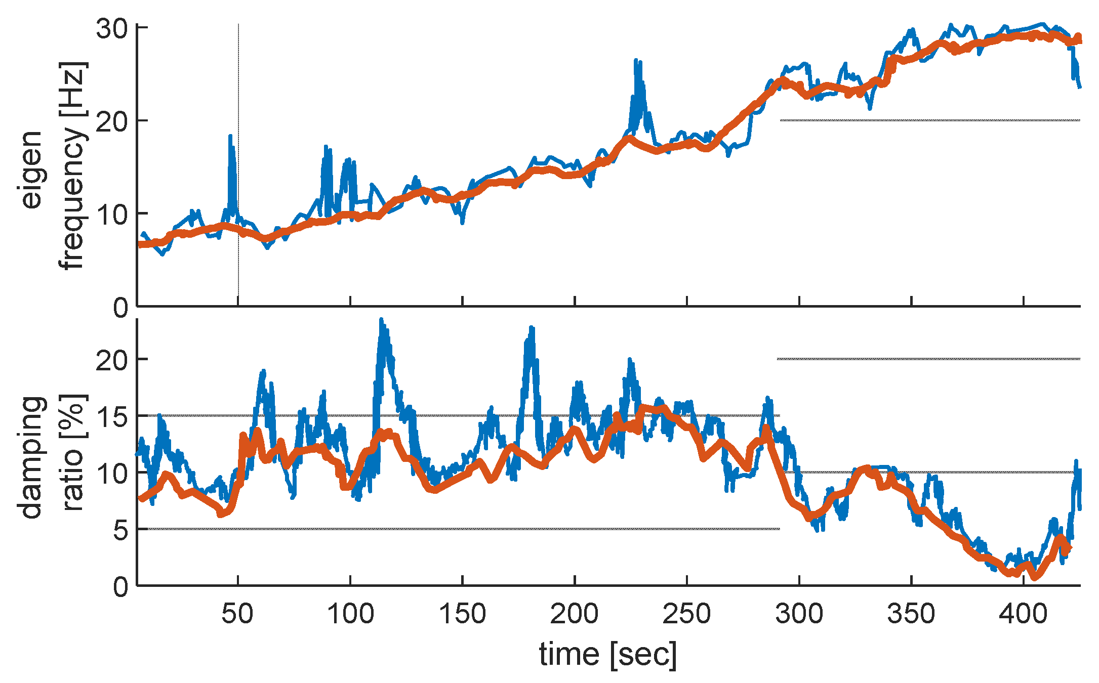
The obtained results are shown in Figure 10. The time-varying character of the modes is clearly visible. The identified modes have been tracked and Figure 13 shows, for instance, the eigenfrequency and damping ratio of the first mode. The dataset contains several short outliers that—even after removing the corresponding samples—resulted in inconsistent estimates using the classical state-of-the-art technique, but it had minimal effect on the proposed methodology; the results are shown without removing the outliers. From these figures, it can be concluded that the regularization approach yields more stable frequency and damping estimates when compared to the classical approach using an exponential window.
6. Conclusions and Future Work
The primary goal of the nonparametric OMA framework is to offer more accurate models that are suitable for understanding, simulation, design, and—indirectly—control. There are many tools available for LTI scenarios, but only a few tools are available for LTV cases.
By using the proposed regularization-based estimation framework, it is possible to significantly improve the estimation quality with respect to the state-of-the-art techniques.
The obtained 2D LTV spectral models can be used to estimate parametric OMA modal models using the classical LTI tools as it has been demonstrated with a simulation example using an exactly known model.
The proposed technique has also been successfully applied to an aerodynamic problem where the use of the method has uncovered the natural and underlying behavior of the lift component in the complex fluid system.
The disadvantage of the proposed method is that the computational cost and memory requirements are significantly higher compared to the state-of-the-art STFT techniques. However, this cost is negligible in applications where (1) the preparation of the measurement setup takes days or even weeks, or (2) no real-time processing is needed.
The authors plan to further enhance the algorithmic part of the methodology in order to find computationally more efficient solutions (such as possible usage of parallel computing) to further increase the performance of the proposed framework and to decrease the memory needs.
Author Contributions
Conceptualization, P.Z.C.; methodology, P.Z.C.; software, P.Z.C.; validation, P.Z.C., M.A. and T.D.T.; formal analysis, P.Z.C., M.A. and T.D.T.; investigation, P.Z.C., M.A. and T.D.T.; resources, P.Z.C., M.A. and T.D.T.; data curation, P.Z.C. and M.A.; writing—original draft preparation, P.Z.C.; writing—review and editing, P.Z.C., M.A. and T.D.T.; visualization, P.Z.C. and M.A.; supervision, P.Z.C. and T.D.T.; project administration, T.D.T.; funding acquisition, T.D.T. All authors have read and agreed to the published version of the manuscript.
Funding
This research was funded by the Vrije Universiteit Brussel, grant number SRP60.
Data Availability Statement
The data presented in this article is available on request.
Conflicts of Interest
The authors declare no conflicts of interest. The funders had no role in the design of the study; in the collection, analyses, or interpretation of data; in the writing of the manuscript; or in the decision to publish the results.
References
- Peeters, B.; De Roeck, G. Stochastic system identification for operational modal analysis: A review. ASME J. Dyn. Syst. Meas. Control 2001, 123, 659–667. [Google Scholar] [CrossRef]
- Rainieri, C.; Fabbrocino, G. Operational Modal Analysis of Civil Engineering Structures; An Introduction and Guide for Applications; Springer: Cham, Switzerland, 2014. [Google Scholar]
- Magalhães, F.; Cunh, Á. Explaining operational modal analysis with data from an arch bridge. Mech. Syst. Signal Process. 2011, 25, 1431–1450. [Google Scholar] [CrossRef]
- Brownjohn, J.; Magalhaes, F.; Caetano, E.; Cunha, A. Ambient vibration re-testing and operational modal analysis of the Humber Bridge. Eng. Struct. 2010, 32, 2003–2018. [Google Scholar] [CrossRef]
- Jing, W.; Hong, Z.; Gang, X.; Erbing, W.; Xiang, L. Operational modal analysis for automobile. In Future Communication, Computing, Control and Management; Lecture Notes in Electrical Engineering; Springer: Cham, Switzerland, 2012. [Google Scholar]
- Møller, N.; Gade, S. Application of Operational Modal Analysis on Car. In SAE 2003 Noise & Vibration Conference and Exhibition; SAE: Warrendale, PA, USA, 2003. [Google Scholar]
- Sichani, M.T.; Ahmadian, H. Identification of Railway Car Body Model Using Operational Modal Analysis. In Proceedings of the 8th International Railway Transportation Conference, Teheran, Iran, 8–9 November 2006. [Google Scholar]
- Morse, T.L.; Williamson, C.H.K. Prediction of vortex-induced vibration response by employing controlled motion. J. Fluid Mech. 2009, 634, 5–39. [Google Scholar] [CrossRef]
- Carberry, J.; Sheridan, J.; Rockwell, D. A Comparison of Forced and Freely Oscillating Cylinders. In Proceedings of the 14th Australasian Fluid Mechanics Conference, Adelaide, Australia, 9–14 December 2001. [Google Scholar]
- Edwins, D. Modal Testing: Theory, Practice and Applications, 2nd ed.; Research Studies Press: Brookline, MA, USA, 2000. [Google Scholar]
- Peeters, B.; Van der Auweraer, H.; Guillaume, P.; Leuridan, J. The PolyMAX Frequency-Domain Method: A New Standard for Modal Parameter Estimation? Shock Vib. 2004, 11, 359–409. [Google Scholar] [CrossRef]
- Calayır, Y.; Yetkin, M.; Erkek, H. Finite element model updating of masonry minarets by using operational modal analysis method. Structures 2021, 34, 3501–3507. [Google Scholar] [CrossRef]
- Reynders, E. System Identification Methods for (Operational) Modal Analysis: Review and Comparison. Arch. Comput. Methods Eng. 2012, 19, 51–124. [Google Scholar] [CrossRef]
- Lyons, R.G. Understanding Digital Signal Processing, 3rd ed.; Prentice Hall: Hoboken, NJ, USA, 2010; ISBN 9780137027415. [Google Scholar]
- Priemer, R. Introductory Signal Processing; World Scientific: Singapore, 1991; ISBN 9971509199. [Google Scholar]
- Oktay, Signals and Systems: A MATLAB® Integrated Approach; CRC Press: Boca Raton, FL, USA, 2014.
- Bartlett, M.S. Periodogram Analysis and Continuous Spectra. Biometrika 1950, 37, 1–16. [Google Scholar] [CrossRef] [PubMed]
- Welch, P.D. The use of Fast Fourier Transform for the estimation of power spectra: A method based on time averaging over short, modified periodograms. IEEE Trans. Audio Electroacoust. 1967, 15, 70–73. [Google Scholar] [CrossRef]
- Zhenkun, L.; Fuhua, M.; Cui, Y.; Mengjia, C. A novel method for Estimating Time of Flight of ultrasonic echoes through short-time Fourier transforms. Ultrasonics 2020, 103, 106104. [Google Scholar]
- Smith, L.; Smith, N.; Kodipaka, S.; Dahal, A.; Tang, B.; Ball, J.E.; Young, M. Effect of the short time fourier transform on the classification of complex-valued mobile signals. SPIE Int. Soc. Optical Eng. 2021, 11756, 2587664. [Google Scholar]
- Matyunina, Z.Y.; Rashevskaya, M. Application of the Short Time Fourier Transform for Calculating Electric Energy Losses under the Conditions of a Non-Sinusoidal Voltage. In Proceedings of the International Ural Conference on Electrical Power Engineering (UralCon), Chelyabinsk, Russia, 22–24 September 2020. [Google Scholar]
- Haiyan, Z.; Yuelong, J.; Baiyang, W.; Yuyun, K. Exercise fatigue diagnosis method based on short-time Fourier transform and convolutional neural network. Front. Physiol. 2022, 13, 965974. [Google Scholar]
- Jont, A.B. Short Time Spectral Analysis, Synthesis, and Modification by Discrete Fourier Transform. IEEE Trans. Acoust. Speech Signal Process. 1977, 25, 235–238. [Google Scholar]
- Peeters, B.; Karkle, P.; Pronin, M.; Van der Vorst, R. Operational Modal Analysis for in-line flutter assessment during wind tunnel testing. In Proceedings of the 15th International Forum on Aeroelasticity and Structural Dynamic, Paris, France, 26–30 June 2011. [Google Scholar]
- Tikhonov, N. On the stability of inverse problems (Об устoйчивoсти oбратных задач). Dokl. Akad. Nauk SSSR 1943, 39, 195–198. [Google Scholar]
- Nikolayevich, V.I. Arsenin, Solution of Ill-posed Problems; Winston & Sons: Washington, DC, USA, 1977; ISBN 0470991240. [Google Scholar]
- Pillonetto, G.; De Nicolao, G. A new kernel-based approach for linear system identification. Automatica 2010, 46, 81–93. [Google Scholar] [CrossRef]
- Buhmann, M.D. Radial Basis Functions: Theory and Implementations; Cambridge University Press: Cambridge, UK, 2009; ISBN 9780521101332. [Google Scholar]
- Rajagopal, V.C.; Ramaswamy, K.R.; Van der Hof, P.M. A regularized kernel-based method for learning a module in a dynamic network with correlated noise. In Proceedings of the IEEE Conference on Decision and Control, Jeju, Republic of Korea, 4–18 December 2020; Volume 2020, pp. 4348–4353. [Google Scholar]
- Ramaswamy, K.R.; Bottegal, G.; Van der Hof, P.M. Learning linear modules in a dynamic network using regularized kernel-based methods. Automatica 2021, 129, 109591. [Google Scholar] [CrossRef]
- Ramaswamy, K.R.; Csurcsia, P.Z.; Schoukens, J.; Van der Hof, P.M. A frequency domain approach for local module identification in dynamic networks. Automatica 2022, 142, 110370. [Google Scholar] [CrossRef]
- Pintelon, R.; Schoukens, J. System Identification: A Frequency Domain Approach; Wiley-IEEE Press: New Jersey, NJ, USA, 2012; ISBN 978-0470640371. [Google Scholar]
- Zadeh, L.A.; Ragazzini, J.R. Frequency analysis of variable networks. Proc. IRE 1950, 38, 291–299. [Google Scholar] [CrossRef]
- Zadeh, L.A. A general theory of linear signal transmission systems. J. Frankl. Inst. 1952, 253, 293–312. [Google Scholar] [CrossRef]
- Csurcsia, P.Z.; Schoukens, J.; Kollár, I. Identification of time-varying systems using a two-dimensional B-spline algorithm. In Proceedings of the 2012 IEEE International Instrumentation and Measurement Technology Conference, Graz, Austria, 13–16 May 2012. [Google Scholar]
- Blanco Alvarez, M.; Csurcsia, P.Z.; Peeters, B.; Janssens, K.; Desmet, W. Nonlinearity assessment of MIMO electroacoustic systems on direct field environmental acoustic testing. In Proceedings of the ISMA 2018—International Conference on Noise and Vibration Engineering and USD 2018—International Conference on Uncertainty in Structural Dynamics, Leuven, Belgium, 17–19 September 2018. [Google Scholar]
- Csurcsia, P.Z.; Peeters, B.; Schoukens, J. The best linear approximation of MIMO systems: Simplified nonlinearity assessment using a toolbox. In Proceedings of the ISMA 2020—International Conference on Noise and Vibration Engineering and USD 2020—International Conference on Uncertainty in Structural Dynamics, Leuven, Belgium, 9–11 September 2020. [Google Scholar]
- Rasmussen, E.; Williams, C.K.I. Gaussian Processes for Machine Learning; MIT Press: Cambridge, MA, USA, 2006; ISBN 026218253X. [Google Scholar]
- Csurcsia, P.Z.; Peeters, B.; Schoukens, J. Tracking the modal parameters of time-varying structures by regularized nonparametric estimation and operational modal analysis. In Proceedings of the 8th IOMAC—International Operational Modal Analysis Conference, Copenhagen, Denmark, 13–15 May 2019; pp. 511–523. [Google Scholar]
- Chen, T.; Ohlsson, H.; Ljung, L. On the estimation of transfer functions, regularizations and Gaussian processes—Revisited. Automatica 2012, 48, 1525–1535. [Google Scholar] [CrossRef]
- Pillonetto, G.; Dinuzzo, F.; Chen, T.; De Nicolao, G.; Ljung, L. Kernel methods in system identification, machine learning and function estimation: A survey. Automatica 2014, 50, 657–682. [Google Scholar] [CrossRef]
- Chen, T.; Ljung, L. Implementation of algorithms for tuning parameters in regularized least squares problems in system identification. Automatica 2013, 49, 2213–2220. [Google Scholar] [CrossRef]
- Marconato, A.; Maarten, S. Tuning the hyperparameters of the filter-based regularization method for impulse response estimation. IFAC-PapersOnLine 2017, 50, 12841–12846. [Google Scholar] [CrossRef]
- Csurcsia, P.Z.; Siddiqi, M.F.; Runacres, M.C.; De Troyer, T. Unsteady Aerodynamic Lift Force on a Pitching Wing: Experimental Measurement and Data Processing. Vibration 2023, 6, 29–44. [Google Scholar] [CrossRef]
- Csurcsia, P.Z.; Peeters, B.; Schoukens, J. The Best Linear Approximation of MIMO Systems: First Results on Simplified Nonlinearity Assessment. In Conference Proceedings of the Society for Experimental Mechanics Series; Springer: Cham, Switzerland, 2020; pp. 53–64. [Google Scholar]
- Tavares, A.; Drapier, D.; Di Lorenzo, E.; Csurcsia, P.Z.; De Troyer, T.; Desmet, W.; Gryllias, K. Automated Operational Modal Analysis for the Monitoring of a Wind Turbine Blade. Structural Health Monitoring 2023: Designing SHM for Sustainability, Maintainability, and Reliability. In Proceedings of the 14th International Workshop on Structural Health Monitoring, Stanford, CA, USA, 12–14 September 2023; pp. 2759–2766. [Google Scholar]
Figure 1.
(Left): the TV IRF of the observed system. (Middle): the ML estimate. (Right): the regularized estimate.
Figure 1.
(Left): the TV IRF of the observed system. (Middle): the ML estimate. (Right): the regularized estimate.

Figure 2.
Overview of the proposed method.

Figure 3.
An experimental illustration to compare the classical (LS) and regularized (RLS) autocorrelation (left) and PSD estimates (right). The LS solution is shown in blue, the regularized solution is shown in red. The numbers in the legend refer to the rms errors between the estimates and the true squared transfer function (shown in black).

Figure 4.
Some selected regularization kernels illustrated on a classical impulse response problem.

Figure 5.
The time-varying output autocorrelation function of the system presented in Figure 1 is shown. The direction represented by the red arrow refers to measurement time where smoothness can be observed. The blue direction refers to the system time where both smoothness and exponential decaying can be observed.

Figure 6.
Illustration of the proposed sliding window technique.

Figure 7.
Flowchart of the recommended processing steps of the proposed methodology.

Figure 8.
Visualization of the simulation and the proposed method for the variance and length estimates.
Figure 8.
Visualization of the simulation and the proposed method for the variance and length estimates.

Figure 9.
The time-varying frequency and damping ratio estimates of the simulation example.

Figure 10.
The time-varying output autocorrelation estimates. On the (left) is the classical windowed correlogram STFT estimate is shown. On the (right) the regularized estimate is shown.
Figure 10.
The time-varying output autocorrelation estimates. On the (left) is the classical windowed correlogram STFT estimate is shown. On the (right) the regularized estimate is shown.

Figure 11.
Illustration of the measurement.

Figure 12.
TV PSD estimates are shown. (left): the classical STFT estimate, (right): the proposed estimate.
Figure 12.
TV PSD estimates are shown. (left): the classical STFT estimate, (right): the proposed estimate.

Figure 13.
Continuous tracking results of the mode located around 20 Hz. The classical approach (blue) is compared to the regularization approach (red).
Figure 13.
Continuous tracking results of the mode located around 20 Hz. The classical approach (blue) is compared to the regularization approach (red).

Disclaimer/Publisher’s Note: The statements, opinions and data contained in all publications are solely those of the individual author(s) and contributor(s) and not of MDPI and/or the editor(s). MDPI and/or the editor(s) disclaim responsibility for any injury to people or property resulting from any ideas, methods, instructions or products referred to in the content. |
© 2024 by the authors. Licensee MDPI, Basel, Switzerland. This article is an open access article distributed under the terms and conditions of the Creative Commons Attribution (CC BY) license (https://creativecommons.org/licenses/by/4.0/).
Share and Cite
MDPI and ACS Style
Csurcsia, P.Z.; Ajmal, M.; De Troyer, T. A Nonparametric Regularization for Spectrum Estimation of Time-Varying Output-Only Measurements. Vibration 2024, 7, 161-176. https://doi.org/10.3390/vibration7010009
AMA Style
Csurcsia PZ, Ajmal M, De Troyer T. A Nonparametric Regularization for Spectrum Estimation of Time-Varying Output-Only Measurements. Vibration. 2024; 7(1):161-176. https://doi.org/10.3390/vibration7010009
Chicago/Turabian StyleCsurcsia, Péter Zoltán, Muhammad Ajmal, and Tim De Troyer. 2024. "A Nonparametric Regularization for Spectrum Estimation of Time-Varying Output-Only Measurements" Vibration 7, no. 1: 161-176. https://doi.org/10.3390/vibration7010009