Objective Function Distortion Reduction in Identification Technique of Composite Material Elastic Properties

Abstract

In studies of structural mechanics, modal analysis, presented in this paper, is an important tool for analyzing the vibration of an object and its frequencies. In modal analysis, different modes of vibration and the frequencies that generate them are considered. The study covers the nondestructive identification of the elastic characteristics of materials, which involves stochastic algorithms and the application of reverse engineering (i.e., the comparison of reference eigenfrequencies with the results of mathematical models). Identification is achieved by minimizing the objective function—the smaller the value of the objective function, the higher the identification accuracy obtained. By changing the parameters of a material’s mathematical model during identification, certain (usually higher order) modes can change places in a natural frequency spectrum. This leads to the comparison of different order eigenfrequencies, slow convergence and poor accuracy of the identification process. The technique involved in this work is the mode-shape recognition of a specimen of material with an “incorrect” set of elastic properties. The results prove that the identification accuracy of a material’s elastic properties can be increased if an “incorrect” set of elastic properties is removed from the identification process. The research covers only numerical research, with a physical experiment simulation.

1. Introduction

First, we would like to talk about finite element analysis. Wang and Inman [1] discussed finite element analysis and conducted an experimental study of the dynamic properties of a composite beam with viscoelastic damping. They mentioned that the frequency-dependent behavior of the stiffness and damping of a viscoelastic material directly affects the system’s modal frequencies and damping and results in complex vibration modes and differences in the relative phase of vibration. Zako et al. [2] discussed the finite element analysis of damaged woven fabric composite materials. They mentioned that their proposed analysis can predict microscopic damage, so that the damage modes could also be described. Mishra and Chakraborty [3] developed an updating technique for a finite element model to allow the estimation of constituent-level elastic parameters of fiber reinforced plastics (FRP) plates. Their technique suggests a viable option for the nondestructive characterization of such FRP structures at the constituent material level.

Next, we would like to mention magnetorheological composites. Yarali et al. [4] discussed the modeling and dynamic finite element analysis of magnetorheological elastomer composites. They mentioned that increasing the magnetic field could lead to an increase in the storage modulus of the magnetorheological elastomer plates. Also, this could consequently increase the values of natural frequencies similar to storage modulus and changing loss factors.

Next, we would like to talk about the modal analysis methods and techniques. A review of operational modal analysis techniques for in-service modal identification is given by Zahid et al. [5]. They mentioned, that the techniques used for modal analysis are experimental modal analysis (EMA), operational modal analysis (OMA) and a less known technique called impact synchronous modal analysis (ISMA), which is a new development. Eliminating the Influence of Harmonic Components in Operational Modal Analysis is given by Jacobsen et al. [6]. They describe a new method based on the well-known Enhanced Frequency Domain Decomposition (EFDD) technique for eliminating these harmonic components in the modal parameter extraction process. Vibration analysis of structures by component mode substitution is given by Benfield and Hruda [7]. They mentioned, that the improvement in accuracy obtained by using interface-loaded-component modes decreased as the number of component modes increased. A general method for the modal decomposition of the equations of motion of damped multi-degree-of-freedom-systems is presented by Stanoev [8]. A novel five-variable refined plate theory for vibration analysis of functionally graded sandwich plates is given by Bennoun et al. [9]. They mentioned, that by dividing the transverse displacement into bending, shear, and thickness stretching parts, the number of unknowns and governing equations of the present theory is reduced, and hence, makes it simple to use. New developments in the analysis of vibrational spectra on the use of adiabatic internal vibrational modes analysed by Cremer et al. [10]. They presented a way of analyzing calculated vibrational spectra in terms of internal vibrational modes associated with the internal coordinates used to describe geometry and conformation of a molecule.

Next, we would like to mention the identification and characterization of elastic properties. Tam [11] reviewed the identification of elastic properties utilizing nondestructive vibrational evaluation methods. He mentioned that the following gaps are worthy of future study: Simplex, Newton, BFGS, Gauss-Newton and SQP. Tam et al. [12] discussed the identification of the material properties of composite materials using nondestructive vibrational evaluation approaches. They stated that the rate of convergence was the main concern involving genetic algorithms. Alfano and Pagnotta [13] described a nondestructive technique for the elastic characterization of thin isotropic plates. Their procedure allows well-known sonic resonance methods for the elastic characterization of homogeneous isotropic materials to be extended to square thin plate specimens. A precise nondestructive damage identification technique for long and slender structures based on modal data was given by Stache et al. [14]. They demonstrated that to detect small damage levels, such as crack depth/diameter ratios less than 10 percent, it is essential to involve the modal data of local modes with adequate measurement precision.

Now, we would like to emphasize the modeling part. Strait et al. [15] described modeling elastic properties in finite-element analysis (FEA). They mentioned that a relatively coarse approach to modeling elastic properties might be adequate for an analysis to assess gross patterns of deformation qualitatively, but more precision may be required if the goal of the FEA is to extract strain data for quantitative analysis. He et al. [16] discussed the characterization of the stress–strain behavior of composites using digital image correlation and finite element analysis. They mentioned that the unknown constitutive properties are determined through minimization of the squared difference between the correlation-measured digital image and the FEM-calculated strains. Viala et al. [17] described the identification of the anisotropic elastic and damping properties of complex-shaped composite parts using an inverse method based on finite element model updating and 3D velocity field measurements.

Studies that focus on the genetic/evolutionary algorithm should be mentioned. Andrzej and Stanislaw [18] described evolutionary algorithm-based methods used to solve global optimization problems. Charbonneau [19] introduced genetic algorithms (GA) for numerical optimization. He mentioned that the use of a genetic algorithm can solve anything that can be formulated as a minimization/maximization task and, in principle, anything that can be described by an equation. An evolutionary algorithm for global optimization, DE/EDA (differential evolution and estimation of distribution algorithm), was presented by Sun et al. [20]. They created/gave a solution by DE/EDA offspring generation scheme in which local information and global information are incorporated.

Finally, we would like to mention the objective function in global optimization problems. Vagaská et al. [21] described selected mathematical optimization methods for solving problems in engineering practice. They mentioned that optimization is applied to process control at all levels, including those of elementary processes, technological processes, and production processes, as well as to the control of processes of strategic importance. Berbecea et al. [22] described a parallel multi-objective efficient global optimization, the finite element method in optimal design and model development. They mentioned that the final surrogate models can be used to determine the sensitivity for each point of the front and, obviously, as predictors of the objective functions that can be used to compute the Pareto frontier. Hofmeister et al. [23] presented finite element model updating using deterministic optimization, a global pattern search approach. Since metaheuristic optimizers (metaheuristic algorithms are the predominant class of optimizers for global optimization problems) need a high amount of objective function evaluations due to their probabilistic search pattern, and derivative-based local optimizers require restarts with randomized start vectors, both approaches are computationally expensive. Cappelli et al. [24] described the multiscale identification of the viscoelastic behavior of composite materials through a nondestructive test. They characterized the viscoelastic behavior of a composite material at each pertinent scale. The characterization of composite elastic properties by means of a multiscale, two-level inverse approach was given by Cappelli et al. [25]. They characterized the elastic properties of a composite material at both the mesoscopic (ply-level) and microscopic (constitutive-phases-level) scales. Montemurro et al. [26] described the identification of the electromechanical properties of piezoelectric structures through evolutionary optimization techniques. They presented a nondestructive method to predict the whole three-dimensional set of electromechanical properties of active plate structures.

We would also like to mention that in this work, the standard GA is applied to a simple elastic structure. As the next step, the physical part will be considered in future experiments. After this review of the known literature, we would like to present our problem formulation.

2. Problem Formulation

Composite materials have constant utilization growth in many industries, such as aerospace, aviation, marine, automotive, military, architecture, energy production, sports and many others. Their increased stiffness and strength properties allow the construction of lightweight components at a reasonable cost. Composite materials are generally defined as the combination of two or more different materials, each retaining its own properties. The result is a new material with properties that cannot be achieved with either component alone.

Designers are constantly faced with the challenges of knowing the mechanical properties of products, which depend on the resin and fiber content, independent layer properties and orientation of orthotropy. Conventional techniques do not always allow generalized material properties to be obtained accurately due to the specific requirements of a particular method. They are restricted by specimen shape and size or require expensive and cumbersome equipment and are destructive. Nondestructive identification techniques, which are quick and comparatively inexpressive, offer a different approach to knowing the material properties.

Nowadays, digital-physical and optimization combination identification technologies for material elastic characteristics intended for industrial purposes are constantly being improved. The main shortcoming of existing technologies is that the elastic characteristics of composite materials are identified with insufficient accuracy.

Despite the aforementioned shortcomings, the technology is intensively developed worldwide in order to create an engineering tool that allows investigators to find all the elastic characteristics of the desired material quickly and with sufficient accuracy. The main idea of identifying the elastic characteristics of a material is to change the finite element model of the material in such a way that its results converge toward the results of the physical vibration experiment.

The experiments performed on various materials showed the shortcomings of the conventional technology of identifying the elastic properties of materials using stochastic algorithms. A method to improve the accuracy of the identification of elastic properties of materials is proposed in this article. The technology utilized in this research is nondestructive and can therefore be applied directly in production.

A hypothesis is raised that during the process of identification, the natural frequencies of the specimen may change their sequence in the spectrum due to a particular (guessed) set of elastic properties. This would distort the value of the objective function and decrease the accuracy of the result because modes of different orders would be compared.

During identification, some modes (usually higher order) can change their position in the natural frequency spectrum compared to physical experimental results. This results in a comparison of the frequencies of different modes in the objective function during the calculations. When this happens, the true value of the objective function becomes distorted and the overall accuracy of the solution suffers. To avoid inaccuracies, it is necessary to check whether the modes remain in “their own” places before calculating the value of the objective function.

To illustrate this phenomenon, an abstract orthotropic material with dimensionless properties was selected. Using finite element method (FEM) software (software version v8; manufacturer: Ansys, Inc.; location: 2600 Ansys Dr Canonsburg, PA, 15317, USA), a mathematical model of the specimen was created and natural frequencies were extracted. After performing the identification procedure and comparing the physical and numerical experimental results, one can see that the 15th mode has changed its shape. These shapes of the 15th mode are shown in Figure 1.

After substituting the values of one of the possible guesses into the mathematical model in the process of identifying the elastic characteristics of the material, it is clear that the 15th mode has acquired a different shape. In this case, a discrepancy in the objective function arises due to the rearrangement of mode frequencies in the spectrum.

The limitations of the model should also be mentioned. In our theoretical model, the deformations are infinitesimally small and the deformation process is isothermal and without viscous elastic effect. Additionally, we would like to mention that thermodynamic restrictions were analyzed in an article by Cappelli et al. [24], who mentioned that the thermodynamic requirements related to the viscoelastic behavior of the matrix (the set of nonlinear constraints) must be considered. Now, we would like to talk about methodology.

3. Methodology

Presently, there is no universal method of undertaking the main and most popular task of identifying the elastic characteristics of many materials without any essential suitable changes. This is caused by the samples used, namely their size, shape and other geometric characteristics. The technology proposed in this article offers the usual material elastic characteristics identification algorithm supplemented with a tool to improve identification accuracy. According to the tests of the proposed technology, and on the basis of global practice, accuracy improvement results are submitted.

For the identification of material elastic characteristics, a genetic algorithm was selected instead of deterministic algorithms. Deterministic algorithms were rejected due to unknown objective function gradients and high computational resource requirements. GA is a search method belonging to the stochastic algorithm family that simulates natural evolution according to the theory proposed by Charles Darwin in 1858.

Properly tuned genetic parameters have a significant influence on the precision of the solution of optimization problems using genetic algorithms—number of generations, crossover and mutation probability values. These values must be chosen based on the algorithm operation tests. Genetic parameters for the material properties identification problem are chosen individually according to the performed numerical experiments and the context of global practices.

The proposed technology was tested in two phases. In the first phase, the elastic characteristics of the materials were identified without recognition of “incorrect” sets of elastic properties. The second step included identification that involved the recognition and rejection of “incorrect” sets.

3.1. Genetic Algorithm as a Global Solver for the Identification Problem

A schematic diagram of the principle of evolutionary algorithms is shown in Figure 2, which shows the typical stages of evolution, such as genetic operations, selection and population replacement, after which the population evolves.

Because GAs are related to evolutionary biology and informatics, they have inherited the specific terms listed below.

Chromosome. A chromosome is a possible solution to an optimization problem. It is composed of genes that are either finite strings or structures that have their own hierarchies. GA genes are built out of binary strings consisting of 0 and 1.

Fitness function. The fitness function shows the fitness of each individual, while the optimal solution of the problem is sought by maximizing or minimizing its value. It should be noted that the fitness function is not analogous to the objective function, as it is more complex. A fitness function is a type of objective function that quantifies whether a solution is optimal. Individuals selected according to the fitness function are crossed over among themselves and further mutated before a new generation is generated.

Population. A population is a set of individuals distributed over the search space. GAs are copulatory because they search for an optimal solution, beginning from multiple starting points.

Generation. A generation is a population of individuals at one particular step (iteration). During GA optimization, the generations are updated until an optimal solution is found or until a given number of generations limit is reached.

Genetic operators. Genetic operators modify individuals in such a way that the entire possible search space can be explored. The mutation operator is a binary genetic operator for moving a chromosome to a new location in the search space. The crossover or recombination operator is designed to create two new individuals from two already existing parents. New individuals inherit some of the characteristics of their parents.

The main stages and processes of GAs are shown in Figure 3. The top shows whether the stage is necessary for the normal course of evolution and the bottom indicates the stage results of the particular step.

Mapping

The concept of mapping is borrowed from evolutionary biology, in which evolution takes place at the genetic level (the genotype) and selection takes place at the physical-biological level (the phenotype). During evolution, the optimal structure of an organism is found by changing its genotype; the genetic material is then coded into a phenotype representing proteins. This shows that the mapping aims to map the structure of the search space to the solution space and vice versa.

Thus, if there is a difference in the GA between the search (binary B) and the solution space (real number R), then a mapping procedure is needed to define that difference. If a chromosome with a certain number of bits $b_i$ is a binary expression of a real number $x\in R$ in the interval $x\in \left[x_{\min },x_{\max }\right]$, then the mapping function $M\left(b_1...b_l\right)$ is:

$$M\left(b_1...b_l\right)=x_{\min }+\frac{x_{\min }-x_{\max }}{2^l+1}\left({\sum }_{j=0}^{l-1}{b}_{l-j}\cdot 2^j\right).$$

(1)

In other algorithms, such as evolutionary strategies and evolutionary programming, there is no distinction between search and solution spaces.

3.2. Global Optimization Problem Formulation

The goal of global optimization is to locate the global extremum of an objective function in a given area of interest. The assumption is made that the objective function requires a lot of effort to evaluate; therefore, information from the search sequence is used to plan the next step. This means that additional computations, which may be effortful, are required to determine the next search point. Problems with simple objective functions do not require global optimization algorithms.

The optimization problem is mathematically formulated as the search for the minimum value of the objective function:

$$\begin{array}{c}\min F\left(\mathbf{x}\right)\\ x\in R^n\end{array}.$$

(2)

where $F\left(\mathbf{x}\right)$ is objective function and $\mathbf{x}\in R^n$ is a feasible search region. A vector $\mathbf{x}$ with a certain number of components describes the design variables. Some of the design variables may be discrete or limited, therefore $\mathbf{X}$ is used to denote the domain of these design variables.

To minimize an objective function $F\left(\mathbf{x}\right)$ in feasible region $\mathbf{X}$ is the goal and can be written:

$$\mathrm{m}\mathrm{i}\mathrm{n}\left\{F\left(\mathbf{x}\right)\vee \mathbf{x}\in \mathbf{X}\subseteq R^n\right\}$$

(3)

The objective function can be described as

$$F\left(\mathbf{x}\right):{\mathbf{X}}_0\subseteq R^n\to R.$$

(4)

The feasible region ${\mathbf{X}}_0$ can be described as

$${\mathbf{X}}_0=\left\{\mathbf{x}\in \mathbf{X}\vee F_i\left(\mathbf{x}\right)\ge 0\right\}\ne 0,$$

(5)

where $F_i:X_i\to R$, $\varnothing \ne X_i\subseteq R^n$, $X={\prod }_{i=1}^p{X}_i$ and $i=\mathrm{1,2},...,p$; the optimization problem can then be formulated as the following:

$$\min \left\{F\left(\mathbf{x}\right)\vee \mathbf{x}\in \mathbf{X},F_i\left(\mathbf{x}\right)\ge 0\right\},$$

(6)

where $i=\mathrm{1,2},...,p$.

As the problem discussed in this article has constraints, the design variables have to be described as belonging to a feasible design space:

$$\mathbf{x}\in \mathbf{X}\subset R^n.$$

(7)

Finally, the optimization problem, including equality and inequality constraints, obtains the following form:

$$\min \left\{F\left(\mathbf{x}\right)\vee \mathbf{x}\in \mathbf{X},F_i\left(\mathbf{x}\right)\ge 0,i\in \mathbf{I},h_j\left(\mathbf{x}\right)=0,j\in \mathbf{J},g_l\left(\mathbf{x}\right)=0,l\in \mathbf{L}\right\},$$

(8)

where I, J and L are indexed sets.

The problem solved in this article falls into the basic engineering category of bounded non-linear single-objective optimization problems; therefore, the objective function $F$ is scalar:

$$\min F\left(\mathbf{x},\mathbf{k}\right),$$

(9)

where $F\left(\mathbf{x},\mathbf{k}\right)\in R,\mathbf{x}\in R^n,\mathbf{k}\in R^m$ and design vectors $\mathbf{x}$ and $\mathbf{k}$ are multidimensional.

The finite element method is employed in a complicated structure analysis. The object under analysis is discretized into a limited number of rectangular or triangular elements. This method entails resolving the structure’s overall mass and stiffness matrix. The classical finite element method equation for calculating eigenfrequencies has the following form:

$$\det \left(\left[\mathbf{K}\right]-{\omega }^2\left[\mathbf{M}\right]\right)=0,$$

(10)

where $\left[\mathbf{K}\right]$ is the global stiffness matrix, $\left[\mathbf{M}\right]$ is the mass matrix of finite element model, and $\omega$ is the angular speed (angular frequency). Eigenvalue $\lambda$ is equal to ${\omega }^2$.

The vibration model data are divided into known (measured) variables and unknown parameters, i.e., elastic characteristics, in identifying the problem formulation. The solution to the identification problem is obtained from the measured independent parameters of the model. These parameters are length, width, thickness $\left(a,b,h\right)$, and frequencies, which are reduced to a single angle $\gamma$ for a single layer material. The variable vector $\mathbf{x}$ is a set of geometric parameters and frequencies:

$$\mathbf{x}={\{a,b,h,\gamma \}}^T.$$

(11)

The global stiffness matrix $\mathbf{K}$ is a function of elastic modulus $E$, shear modulus $G$ and Poisson’s ratio $\nu$ (the number of elastic characteristics depends on the material).

$$\mathbf{k}={\{E_1,E_2,G_{12},{\upsilon }_{12},G_{13},G_{23},E_3,{\nu }_{13},{\nu }_{23}\}}^T.$$

(12)

The optimization problem of interest finally obtains the following form:

$$\min F=F\left(\mathbf{x},\mathbf{k}\right).$$

(13)

Including limitations:

$$\begin{array}{c}\underset{\_}{g_i}\left(\mathbf{k}\right)\le {\overline{g}}_{𝚤},i=\mathrm{1,2},3,...,m_1\\ \underset{\_}{h_i}<{\overline{h}}_{𝚤}\left(\mathbf{k}\right),i=\mathrm{1,2},3,...,m_2\\ \underset{\_}{k_i}\le k_i\le {\overline{k}}_{𝚤},i=\mathrm{1,2},3,...,m_3\end{array},$$

(14)

where $m_1$, $m_2$, $m_3$ are constants. The lower and upper dashes represent the lower and upper bounds, respectively. The objective function $F$ and the state variables $g_i$ and $h_i$ can be linear or non-linear functions of the design variable $k_i$.

The objective function of the identification problem has the following form:

$$F\left(\mathbf{x},\mathbf{k}\right)={\sum }_{i=1}^n{\left(\frac{f_i^N-f_i^{FEM}}{f_i^N}\right)}^2,$$

(15)

where $f_i^{FEM}$ is the calculated natural frequency, $f_i^N$ is the experimentally obtained natural frequency and $n$ is the covered part of the spectrum. The natural frequencies are the state variables of the problem, and the design variables are the elastic characteristics of the material.

The first four elastic coefficients are sufficient to describe an isotropic material. The experiment (physical or digital) provides a sufficient part of the eigenfrequencies of the structure. The frequency equation is written as follows:

$$f_i=F_i\left(\mathbf{x},\mathbf{k}\right),i=\mathrm{1,2},...,n,$$

(16)

where n is the part of the spectrum of real values, $f_i$ is the nth eigenfrequency.

3.3. Mathematical Models of Materials

In the body under the influence of external effect (load), internal forces (tensions) appear. Stresses are the result of the mutual interactions of individual parts of the body divided by sections and are usually associated with the law of material behavior that defines its mechanical properties. These laws were derived from practical observations during tests. Geometric changes in a deformable body are characterized by displacements and deformations. Under the influence of external forces, the body deforms and its points shift relative to each other. Displacements and deformations are defined in the elasticity matrix.

The relationship between the stresses and strains of a physically linear body, also known as Hooke’s law, is expressed as follows:

$$\{\mathsf{\epsilon }\}=\left[\mathbf{C}\right]\{\mathsf{\sigma }\}\Rightarrow \left\{\begin{array}{c}{\epsilon }_{11}\\ {\epsilon }_{22}\\ {\epsilon }_{33}\\ {\epsilon }_{12}\\ {\epsilon }_{13}\\ {\epsilon }_{23}\end{array}\right\}=\left[\begin{array}{cccccc}{C}_{11}& C_{12}& C_{13}& C_{14}& C_{15}& C_{16}\\ C_{21}& C_{22}& C_{23}& C_{24}& C_{25}& C_{26}\\ C_{31}& C_{32}& C_{33}& C_{34}& C_{35}& C_{36}\\ C_{41}& C_{42}& C_{43}& C_{44}& C_{45}& C_{46}\\ C_{51}& C_{52}& C_{53}& C_{54}& C_{55}& C_{56}\\ C_{61}& C_{62}& C_{63}& C_{64}& C_{65}& C_{66}\end{array}\right]\left\{\begin{array}{c}{\sigma }_{11}\\ {\sigma }_{22}\\ {\sigma }_{33}\\ {\sigma }_{12}\\ {\sigma }_{13}\\ {\sigma }_{23}\end{array}\right\}.$$

(17)

This relation of deformations is satisfied in the case that no plastic deformation occurs, the deformations are infinitesimally small and the deformation process is isothermal. These conditions make it possible to apply the principle of the action of independent forces—the concept of the state of linear tension and net shear when the deformation of a three-dimensional body in the chosen direction is determined.

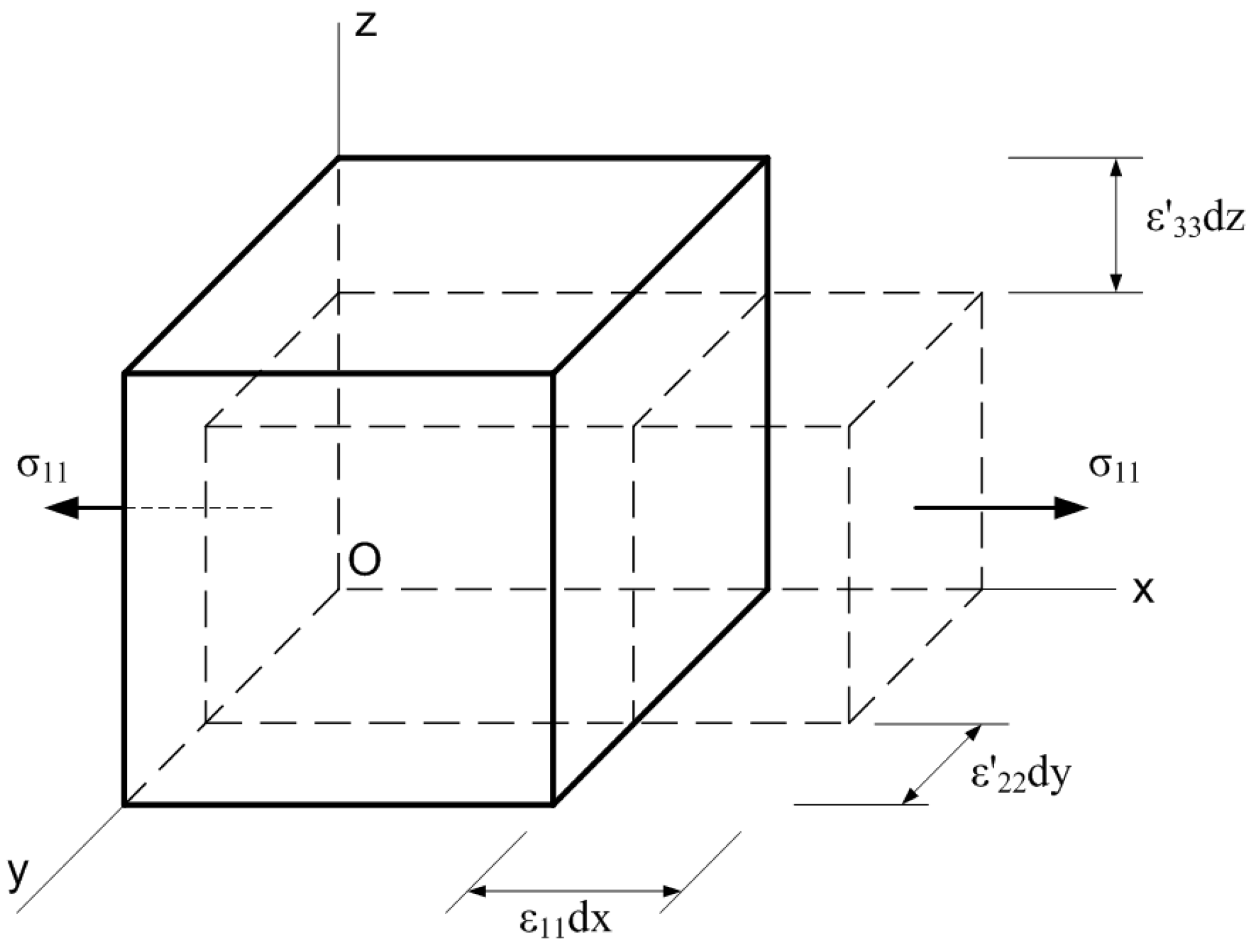
As an example, let us take a perfectly elastic isotropic body whose elastic properties are described by only two independent constants, $E$ and $G$, or $G$ and $\nu$ or $E$ and $\nu$. They do not depend on the coordinates of the body point or on the selected coordinate system. In this case, Equation (18) becomes quite simple. Assume that there is only one normal stress ${\sigma }_{11}$, the coefficients $C_{i1},C_{i2},...,C_{i6}$ are known and all other stresses are equal to zero (Figure 4). If an ideal rectangular parallelepiped is stretched in the direction of the X axis, its deformation would be ${\epsilon }_{11}={\sigma }_{11}/E$.

Transverse deformation manifests as a relative change in the transverse dimensions of a stretched rod. Its direction is opposite to $dx$:

$${\epsilon }_{22}^{’}={\epsilon }_{33}^{’}=-{\mathsf{\nu }\mathsf{\epsilon }}_{11}=\frac{-\nu }{E}{\sigma }_{11}.$$

(18)

Poisson’s ratio is a dimensionless mechanical characteristic/indicator of the material, the modulus of the ratio of the transverse deformation of the tensile or compressive layers of the structural element to the longitudinal deformation. For materials, Poisson’s ratio remains constant as long as the strains are proportional to the stresses. Under the action of only one stress ${\sigma }_{11}$, the initial vertical angles between the edges of the elementary parallelepiped of a homogeneous isotropic material do not change, so the deformations ${\epsilon }_{12},{\epsilon }_{13}$ and ${\epsilon }_{23}$ are equal to zero. In this case, the coefficients of the elasticity matrix are:

$$C_{11}=\frac{1}{E}, C_{21}=C_{31}=\frac{-\nu }{E}, C_{41}=C_{51}=C_{61}=0.$$

(19)

Analogously, acting only on ${\sigma }_{22}$ or ${\sigma }_{33},$ stresses yield to:

$$C_{22}=C_{33}=\frac{1}{E}, C_{12}=C_{33}=\frac{-\nu }{E}, C_{42}=C_{52}=C_{62}=C_{43}=C_{53}=C_{63}=0.$$

(20)

If the elementary parallelogram were subjected to tangential stresses ${\sigma }_{12}$ only, net shear would act in the plane $\mathrm{O}xy$ (Figure 5).

The angular strain in the $0xy$ plane is ${\epsilon }_{12}={\sigma }_{12}/G$. Under the action of ${\sigma }_{12}$ tension, the angles in other coordinate planes will not change, i.e., ${\epsilon }_{12}={\epsilon }_{23}=0$, and linear deformations are equal to zero: ${\epsilon }_{11}={\epsilon }_{22}={\epsilon }_{33}={\epsilon }_{12}={\epsilon }_{23}=0$.

When there is only one tangential stress ${\sigma }_{12}$ and the others are equal to zero, the coefficients of the elasticity matrix are:

$$C_{44}=\frac{1}{G}, C_{14}=C_{24}=C_{34}=C_{54}=C_{64}=0.$$

(21)

When all stresses ${\sigma }_{11},{\sigma }_{22},{\sigma }_{33},{\sigma }_{12},{\sigma }_{13},{\sigma }_{23}$ act together:

$$\left\{\begin{array}{c}{\epsilon }_{11}=\frac{1}{E}\left[{\sigma }_{11}-\nu \left({\sigma }_{22}+{\sigma }_{33}\right)\right],\\ {\epsilon }_{22}=\frac{1}{E}\left[{\sigma }_{22}-\nu \left({\sigma }_{11}+{\sigma }_{33}\right)\right]\\ {\epsilon }_{33}=\frac{1}{E}\left[{\sigma }_{33}-\nu \left({\sigma }_{11}+{\sigma }_{22}\right)\right],\end{array}\right., \begin{array}{c}{\epsilon }_{12}=\frac{1}{G}{\sigma }_{12}\\ {\epsilon }_{13}=\frac{1}{G}{\sigma }_{13}\\ {\epsilon }_{23}=\frac{1}{G}{\sigma }_{23}\end{array}.$$

(22)

The mechanical properties of the material (elasticity characteristics) $G$, $E$ and $\nu$ are linked by a relationship known from the mechanics of materials:

$$G=\frac{E}{2\left(1+\nu \right)}.$$

(23)

The inverse Hooke’s law is obtained by expressing stresses in terms of strains. Using the yield matrix $\left[\mathbf{D}\right]$, the inverse Hooke’s law is written in matrix form as follows:

$$\{\mathsf{\sigma }\}=\left[\mathbf{D}\right]\{\mathsf{\epsilon }\}\Rightarrow \left\{\begin{array}{c}{\sigma }_{11}\\ {\sigma }_{22}\\ {\sigma }_{33}\\ {\sigma }_{12}\\ {\sigma }_{13}\\ {\sigma }_{23}\end{array}\right\}=\frac{1}{E}\left[\begin{array}{cccccc}{D}_{11}& D_{12}& D_{13}& D_{14}& D_{15}& D_{16}\\ D_{21}& D_{22}& D_{23}& D_{24}& D_{25}& D_{26}\\ D_{31}& D_{32}& D_{33}& D_{34}& D_{35}& D_{36}\\ D_{41}& D_{42}& D_{43}& D_{44}& D_{45}& D_{46}\\ D_{51}& D_{52}& D_{53}& D_{54}& D_{55}& D_{56}\\ D_{61}& D_{62}& D_{63}& D_{64}& D_{65}& D_{66}\end{array}\right]\left\{\begin{array}{c}{\epsilon }_{11}\\ {\epsilon }_{22}\\ {\epsilon }_{33}\\ {\epsilon }_{12}\\ {\epsilon }_{13}\\ {\epsilon }_{23}\end{array}\right\}.$$

(24)

For isotropic material, its yielding matrix would be as follows:

$$\mathbf{D}=\frac{1}{E}\left[\begin{array}{cccccc}1& -\nu & -\nu & 0& 0& 0\\ -\nu & 1& -\nu & 0& 0& 0\\ -\nu & -\nu & 1& 0& 0& 0\\ 0& 0& 0& 2\left(1+\nu \right)& 0& 0\\ 0& 0& 0& 0& 2\left(1+\nu \right)& 0\\ 0& 0& 0& 0& 0& 2\left(1+\nu \right)\end{array}\right].$$

(25)

3.4. Mode Shape Recognition Algorithm

Mode evaluation is a crucial step before any comparison. The material properties identification technique is based on comparisons of corresponding frequencies. Mode shapes have high importance because they come from physical material behavior.

The recognition of mode shapes in this study is based on the principle of the modal assurance criterion (MAC). MAC is a statistically based method of identifying the differences in mode shapes. This method is sensitive to large differences and considers only mode shapes without involving frequency in comparison. The evaluation of mode shapes is bounded between 0 and 1, and does not indicate orthogonality or validity. A smaller evaluation result indicates that the modes are different.

This work involves a modified MAC to recognize the shape of sample modes and determine their sequence in the spectrum. In MAC, the comparison is performed by analyzing modal vectors in the full or reduced order of FEM. Modifications of MAC in this work include shape recognition by the displacements of the FEM grid points in the direction of the Z axis because it is assumed that since sample side-lengths are hundreds of times greater than the thickness, the sample modes will be located in the XY plane only. By forming a list of normalized values of the displacements of a finite number of points in the direction of the Z axis of a physical specimen (reference) and comparing it with an alike list of a digital specimen (comparable), it is possible to determine mode shape differences and similarities. The lists are built in the form of a two-dimensional matrix. The discrepancy is measured by the number of matching points found during the tests and is called the simple matching rate, expressed as a percentage. Since the number of modes in the process of identifying the material elastic characteristics rarely exceeds 15–20, mode shapes are recognized using a simple linear search algorithm.

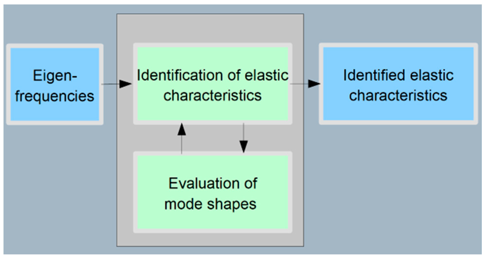
Figure 6 shows the location of the shape recognition part in the material properties identification technology. As can be seen, this part is constantly involved in the identification process of the material elastic characteristics—after calculating the natural frequencies of the specimen with the guessed elastic characteristics of the population, the algorithm checks and sorts the list of natural frequencies before calculating the objective function.

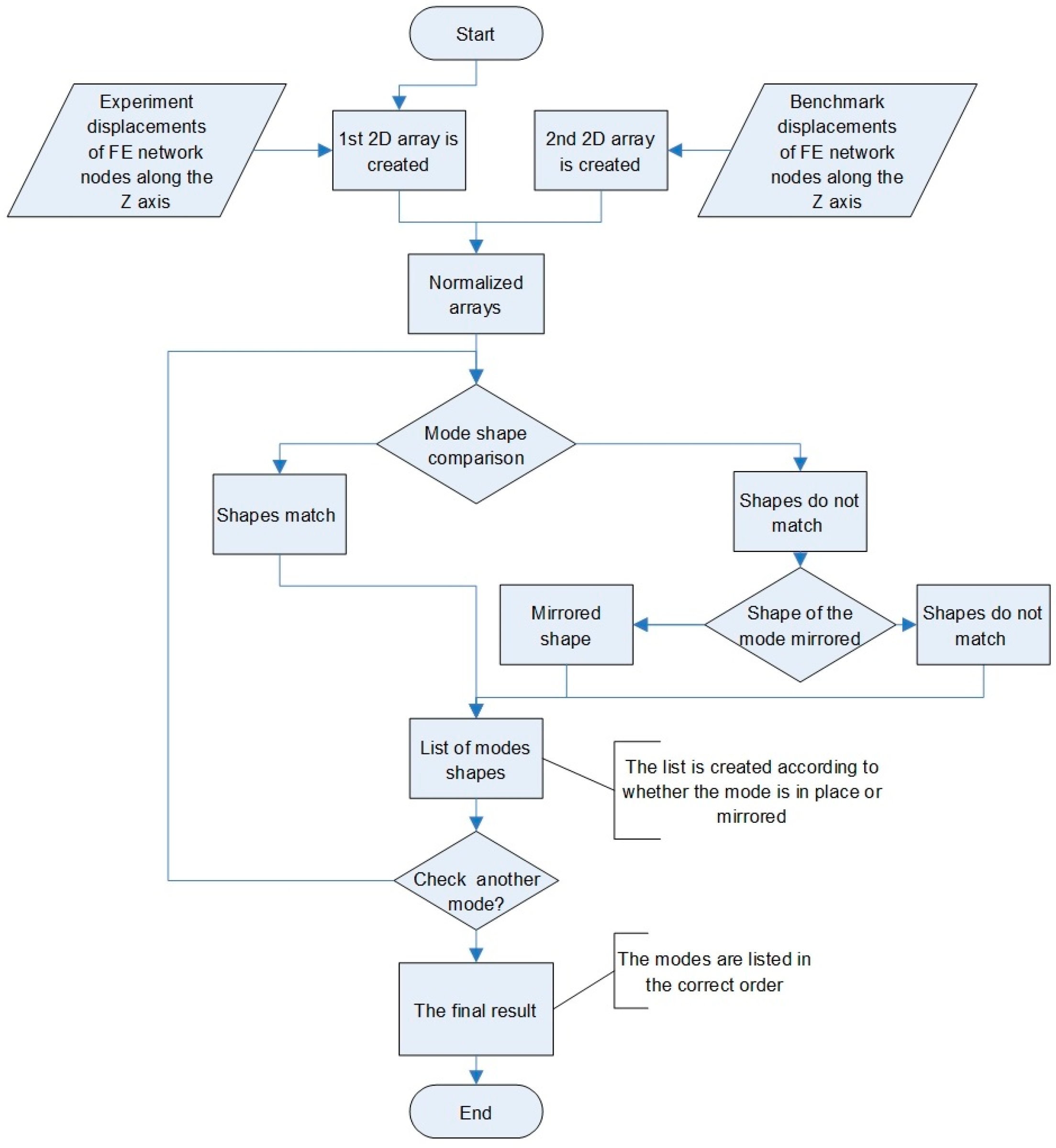
The flowchart of the mode shape recognition algorithm is presented in Figure 7. The Z-coordinate lists of the reference and comparable modes are written into distinct two-dimensional arrays. Next, the arrays are normalized to eliminate the influence of offset values. Each element mesh point in the reference array is then compared with its comparable array. In the logical element of the flow “Does the mode shape match?”, an algorithm for recognizing the mode shape is encoded: if a certain number of values of a certain mode in both arrays coincide, the mode shapes are considered to be the same. If the required number of matching values is not reached, the algorithm searches for matches with the next mode in the sequence, and so on. Then it is moved on to the next mode in the reference list until all the modes necessary in the process of identifying the elastic characteristics of materials have been checked and ordered.

The logical data list provided by the algorithm contains information about the proper mode location, whether the mode has a mirroring pair, and which mode it swapped places with (

Table 1. Logical data list of the mode arrangement for the nth individual.

Row No. of the Mode	Is Location Appropriate?	Appropriate Location	Is Shape Mirrored?	Which Mode Swapped with
1	1	10...000	0	00...000
2	1	01...000	0	00...000
...	...	...	...	...
n − 2	0	00...010	0	00...100
n − 1	0	00...100	0	00...010
n	1	00...001	0	00...000

). The example shows the mode arrangement of a specimen obtained with the guessed elastic characteristics of the nth individual. In the identification process, sequence mode n-2 has migrated from its reference position. Its original position is defined in the column “Appropriate location”, where it can be seen that the reference position is one before the last. With a particular set of material properties, the mode has taken up a position two before the last and does not correspond to the original. These positions are coded using zeroes and ones: the 15th mode’s original position has unity in the code sequence “0000000000000010”, while the incorrect position is coded as “0000000000000100”.

According to this logical list, the algorithm sorts the modes into the required order and provides a “correct” list to the objective function calculation for the genetic algorithm (GA).

4. Results

Increasing the accuracy of the objective function results for the identification of elastic properties (for example, Poisson’s ratio) has a direct impact on the overall accuracy of the solution to the problem of identifying the elastic properties of materials. In order to avoid distortion of objective function due to the mode shape transition effect, a procedure has been developed that recognizes mode shapes and determines their proper position in the spectrum corresponding to the natural experiment results.

4.1. Simple Matching Coefficient of Mode Shape Recognition Algorithm

In order to fine-tune the accuracy of the mode shape recognition algorithm, several tests were carried out and the value of the matching coefficients was determined experimentally.

The simple matching coefficient (SMC) is the statistics used to compare the similarity and diversity of sample sets—Verma and Aggarwal [27,28]. Given two objects A and B, each with n binary attributes, SMC is defined as:

$$SMC=\frac{number of matching attributes}{total number of attributes}=\frac{M_{00}+M_{11}}{M_{00}+M_{11}+M_{01}+M_{10}}.$$

(26)

where M₀₀ is the total number of attributes where A and B both have a value of 0. M₁₁ is the total number of attributes where A and B both have a value of 1. M₀₁ is the total number of attributes where A has value 0 and B has value 1. M₁₀ is the total number of attributes where A has value 1 and B has value 0.

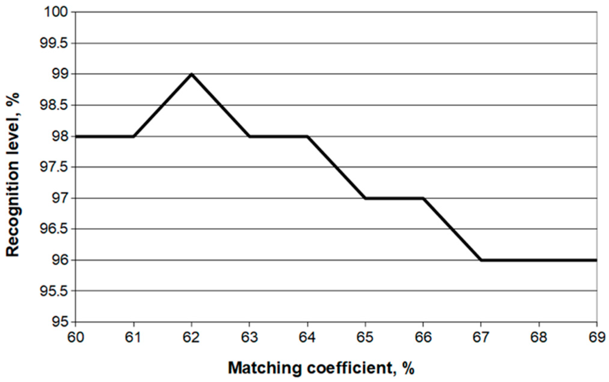
The values of the SMC and the recognized number of modes from the selected spectrum are shown in Figure 8. As can be seen, the greatest number of modes is recognized when the SMC value is 60%.

According to the results of the first approach, the highest accuracy was achieved when the values of the SMC were between 60% and 70%. To fine-tune the algorithm for more precise results, narrower boundaries were chosen for the SMC, and the test led to 62%, as shown in Figure 9.

During the experiments, it was noted that the shape of mode did not correspond to the reference, but was determined as having rotated 90° or 180°. These modes are mirrored to reference spectrum modes (Figure 10). Mirrored modes have the same frequency, but their orientation differs from the reference. They do not skew the objective function but must be determined so as not to be excluded by the algorithm as inappropriate.

The mirrored mode can be recognized by turning it around the Z axis every 90° and comparing it with the reference. The list of points in the comparable mode is transformed by turning the mode shape by 90° and comparing it with the reference. If the shape of the modes does not match, the list is rotated again by 90°. If the mode shape does not match after the second transformation, it is concluded that the modes are different.

4.2. Identification of Elastic Characteristics of Layered Composite Material Using Mode Shape Recognition

If the main directions of the orthotropy of the material layers coincide, such a material is called unidirectional. In general, the properties of a layered material consisting of unidirectional layers are described by nine independent elastic characteristics:

$$\left[\begin{array}{c}{\epsilon }_{11}\\ {\epsilon }_{22}\\ {\epsilon }_{33}\\ {\epsilon }_{23}\\ {\epsilon }_{13}\\ {\epsilon }_{12}\end{array}\right]=\left[\begin{array}{cccccc}\frac{1}{E_1}& \frac{-{\nu }_{12}}{E_2}& \frac{-{\nu }_{13}}{E_2}& 0& 0& 0\\ \frac{-{\nu }_{12}}{E_1}& \frac{1}{E_2}& \frac{-{\nu }_{23}}{E_2}& 0& 0& 0\\ \frac{-{\nu }_{13}}{E_1}& \frac{-{\nu }_{23}}{E_2}& \frac{1}{E_3}& 0& 0& 0\\ 0& 0& 0& \frac{1}{G_{23}}& 0& 0\\ 0& 0& 0& 0& \frac{1}{G_{13}}& 0\\ 0& 0& 0& 0& 0& \frac{1}{G_{12}}\end{array}\right]\left[\begin{array}{c}{\sigma }_{11}\\ {\sigma }_{22}\\ {\sigma }_{33}\\ {\sigma }_{23}\\ {\sigma }_{13}\\ {\sigma }_{12}\end{array}\right]$$

(27)

The elastic characteristics of the layered unidirectional material here are defined for the entire sample and not for each layer separately. The mathematical model of the material is simplified to a single-layer material; i.e., the properties of the material are described by six independent characteristics of elasticity:

$$\begin{array}{c}{E}_1,{ E}_2=E_3,{\nu }_{12}={\nu }_{13},{\nu }_{23},\\ G_{12}=G_{13}{, G}_{23}=E_2/2\left(1+{\nu }_{23}\right)\end{array}$$

(28)

Bearing in mind the insufficient identification accuracy of Poisson’s ratio and in order to simplify the three-dimensional task, researchers often make assumptions—Frederiksen [29,30]:

$$E_1,E_2=E_3,{\nu }_{12}={\nu }_{13}={\nu }_{23},G_{12}=G_{13}=G_{23}$$

(29)

A test was performed on an abstract orthotropic material with six dimensionless properties: $E_1=1$, $E_2=E_3=0.1$, ${\nu }_{12}={\nu }_{13}=0.3$, ${\nu }_{23}=0.6$, $G_{12}=G_{13}=0.05$, $G_{23}=0.03$ in order to show possible discrepancies, despite the low impact of out-of-plane characteristics on eigenfrequencies due to the specimen thickness (250 mm × 250 mm × 2 mm). The search limits were selected by setting approximately equal intervals in both directions based on their pre-known values. SHELL63 FE, which has bending capabilities, was used; the element permits in-plane and normal loads, and each node of the element has six degrees of freedom. A 5 × 5 rectangular grid density was used to extract eigenfrequencies, for which a converged solution was obtained in ANSYS software (software version v8; manufacturer: Ansys, Inc.; location: 2600 Ansys Dr Canonsburg, PA, 15317, USA) simulating free vibration. The genetic parameters were selected by testing and according to international practice: crossover probability—0.9, mutation probability—0.1, population size—10, and number of populations—250.

Using the known elastic characteristics, the natural frequencies $f_i^N$ of the digital specimen were obtained, which are presented in

Table 2. A case of mode switching.

Mode No.	${\mathit{f}}_{\mathit{i}}^{\mathit{N}}$	${\mathit{f}}_{\mathit{i}}^{\mathit{FEM}}$	i-th Member of the Objective Function
			without Mode Shape Recognition	with Mode Shape Recognition
1	0.03845	0.03848	0.0000007368	0.0000007368
2	0.09225	0.09131	0.0001040511	0.0001040511
...	...	...	...	...
13	0.50313	0.50264	0.0000009640	0.0000009640
14	0.50435	0.50711	0.0000297949	0.0000397792
15	0.50549	0.50754	0.0000163989	0.0000102582
Sum of objective function			0.0004448056	0.0004486493

. The adjacent column shows the natural frequencies $f_i^{FEM}$ of the specimen obtained with the guessed elastic characteristics of the nth individual. It can be seen that the 14th and 15th modes have swapped places in the spectrum, but the frequencies are still in ascending order, so the mismatches will be incorrectly estimated in the objective function.

Without mode shape recognition and correct ordering, the 14th and 15th members of the objective function are calculated by taking adjacent values of the physical specimen and the FEM solution:

$$F_{14}={\left(\frac{f_{14}^N-f_{14}^{FEM}}{f_{14}^N}\right)}^2={\left(\frac{0.50435-0.50711}{0.50435}\right)}^2=0.0000297949,$$

(30)

$$F_{15}={\left(\frac{f_{15}^N-f_{15}^{FEM}}{f_{15}^N}\right)}^2={\left(\frac{0.50549-0.50754}{0.50549}\right)}^2=0.0000163989.$$

(31)

If the mode shapes are arranged according to the mode order of the physical specimen, the above-mentioned members of the objective function are calculated as follows:

$${F’}_{14}={\left(\frac{f_{14}^N-f_{15}^{FEM}}{f_{14}^N}\right)}^2={\left(\frac{0.50435-0.50754}{0.50435}\right)}^2=0.0000397792,$$

(32)

$${F’}_{15}={\left(\frac{f_{15}^N-f_{14}^{FEM}}{f_{15}^N}\right)}^2={\left(\frac{0.50549-0.50711}{0.50549}\right)}^2=0.0000102582.$$

(33)

The difference between the intermediate values of the objective function is 0.000003844, or 0.85%, compared to results involving mode shape recognition. If several pairs of modes were swapped, the solution would be distorted more with respect to the number of swapped modes. If the mode shapes are not properly ordered, an incorrect solution to the identification of elastic properties may be obtained. A similar spectrum of natural frequencies of a numerical specimen can occur with values of elastic characteristics far from the expected solution, but the order of the modes may be consistent.

4.3. Numerical Experimental Results

As the genetic algorithm is a stochastic algorithm, 20 independent calculation cycles were performed in both cases, with and without mode shape recognition, to ensure the reliability of the results. The identification task was solved by involving GA and FEM; the genetic parameters were experimentally determined: crossover probability—0.9, mutation probability—0.1, population size—30, and number of populations—100. A total of 1.2 × 10⁵ independent numerical experiments were carried out. The following figures show that the number of calculation steps (guesses) was sufficient to achieve the expected accuracy of the identification process, which is common in solving engineering problems nowadays.

Figure 11 shows the average values of the objective function—the red curve shows the average values of the objective function in each generation without mode shape recognition, while the green curve shows the average values of the objective function in each generation with mode shape recognition. From the graph, it can be seen that mode shape recognition affects the character of convergence and the mean value of each successive population decreases smoothly. Meanwhile, without mode shape recognition, the convergence is less continuous, and sharp jumps between populations are observed.

The average of the objective function is 0.01051 without mode shape recognition and 0.00988 with recognition; standard deviation 0.06816 and 0.06334, respectively. It can be seen that recognizing inappropriate mode shapes and removing such individuals from the population reduces the mean of the objective function by 0.00063 (6.35%) and the standard deviation by 0.00482 (7.6%). A lower number indicates increased accuracy of the material elastic characteristic identification results.

By using mode shape recognition, the identification error of the elastic characteristics was reduced.

Table 3. Material properties identification results comparison.

Elasticity Parameter	Reference	Without Recognition	Δ1, %	With Recognition	Δ2, %
$E_1$	1	0.99163	0.837	1.002158	0.2158
$E_2=E_3$	0.1	0.098047	1.953	0.101912	1.912
$G_{12}=G_{13}$	0.05	0.0509695	1.939	0.0499175	0.165
$G_{23}$	0.03	0.0320361	6.787	0.027603	7.99
${\nu }_{12}={\nu }_{13}$	0.3	0.293616	2.128	0.296202	1.266
${\nu }_{23}$	0.6	0.561121	6.298	0.548208	8.632

presents the identified elasticity characteristics and errors with and without shape recognition. In the Reference column, the abstract elastic characteristics of the material are given. Table 3 presents the average of the identified elastic characteristics of the material and the percentage of identification error ${\Delta }_i$ (calculated according to Equation (34)).

$${\Delta }_i=\left|\frac{k^{REF}-k^{FEM}}{k^{FEM}}\right|\times 100.$$

(34)

where $k^{FEM}$ represents the calculated and $k^{REF}$ the known elastic characteristics.

As can be seen in Table 3, after involving mode shape recognition, the in-plane elastic characteristics are identified with a higher accuracy. The out-of-plane elastic characteristics are identified with uncertain accuracy because they have a low influence on the natural frequencies of the specimen due to the large ratio between the side length and the thickness of the specimen.

4.4. Key Findings

• The proposed methodology allows us to increase the accuracy of nondestructive identification results. It can be applied to find the material properties of layered complex structures.
• The hypothesis raised about mode swapping phenomena was found to have an effect on the identification accuracy of material elastic characteristics. The hypothesis is confirmed by the fact that the elastic characteristics of materials are identified more accurately if the sets of “inappropriate” modes are removed from the identification process.
• Although complex identification methods are used to determine the elastic characteristics of composites, the identification method used in this paper allows us to identify the aforementioned characteristics with sufficient accuracy. Moreover, this method can be used in areas that require high design and modeling accuracy, such as aviation, the space industry, wind power plants, etc.

The presented model is part of general complex models and will be involved in future studies.

5. Conclusions

The recognition of mode shapes according to the physical experimental data in the material elastic characteristics identification process was analyzed in this study. As mentioned in the problem formulation, a hypothesis was raised that, during the identification process of the elastic properties of materials, natural frequencies of the specimen may change their sequence in the spectrum due to a particular set of elastic properties. Comparative experiments involving mode shape recognition showed an overall identification accuracy increase: $E_1$ by 3.88 times, $G_{12}$ by 11.75 times and ${\nu }_{12}$ by 1.68 times.

The simple match coefficient was used to recognize the mode shape; this shows how many nodes of finite element (FE) mesh Z axis displacements coincide with the corresponding points of the reference. The value of this coefficient was determined experimentally, and the most accurate recognition was found at 62% of the SMC value.

Recognizing inappropriate mode shapes and removing such individuals from the population reduces the mean of the objective function by 0.00063 (6.35%) and the standard deviation by 0.00482 (7.6%).

We would like to mention that the model we present is limited to the specific application of nondestructive identification of the elastic properties of materials using standard GA. Future studies of modal analysis will focus on other approaches and methods, such as the nondestructive evaluation (NDE) approach and wave-based characterization techniques that include the inhomogeneous wave correlation method and the transition frequency characterization method—Chronopoulosa et al. [31]—as well as improving the previous experience with identifying the properties of the material [32,33,34].

References

- Wang, Y.; Inman, D.J. Finite element analysis and experimental study on dynamic properties of a composite beam with viscoelastic damping. J. Sound Vib. 2013, 332, 6177–6191. [Google Scholar] [CrossRef]
- Zako, M.; Uetsuji, Y.; Kurashiki, T. Finite element analysis of damaged woven fabric composite materials. Compos. Sci. Technol. 2003, 63, 507–516. [Google Scholar] [CrossRef]
- Mishra, A.K.; Chakraborty, S. Development of a finite element model updating technique for estimation of constituent level elastic parameters of FRP plates. Appl. Math. Comput. 2015, 258, 84–94. [Google Scholar] [CrossRef]
- Yarali, E.; Farajzadeh, M.A.; Noroozi, R.; Dabbagh, A.; Khoshgoftar, M.J.; Mirzaali, M.J. Magnetorheological elastomer composites: Modeling and dynamic finite element analysis. Compos. Struct. 2020, 254, 112881. [Google Scholar] [CrossRef]
- Zahid, F.B.; Ong, Z.C.; Khoo, S.Y. A review of operational modal analysis techniques for in-service modal identification. J. Braz. Soc. Mech. Sci. Eng. 2020, 42, 398. [Google Scholar] [CrossRef]
- Jacobsen, N.J.; Andersen, P.; Brincker, R. Eliminating the influence of harmonic components in operational modal analysis. In Proceedings of the IMAC XXV Conference, Orlando, FL, USA, 19–22 February 2007. [Google Scholar]
- Benfield, W.; Hruda, R. Vibration analysis of structures by component mode substitution. AIAA J. 1971, 9, 1255–1261. [Google Scholar] [CrossRef]
- Stanoev, E. A modified modal analysis method for damped multi-degree-of-freedom-systems in structural mechanics. Z. Angew. Math. Mech. 2015, 95, 566–588. [Google Scholar] [CrossRef]
- Bennoun, M.; Houari, M.S.A.; Tounsi, A. A novel five-variable refined plate theory for vibration analysis of functionally graded sandwich plates. Mech. Adv. Mater. Struct. 2016, 23, 423–431. [Google Scholar] [CrossRef]
- Cremer, D.; Larsson, J.A.; Kraka, E. New developments in the analysis of vibrational spectra on the use of adiabatic internal vibrational modes. In Theoretical and Computational Chemistry; Parkanyi, C., Ed.; Elsevier: Amsterdam, The Netherlands, 1998; pp. 259–327. [Google Scholar] [CrossRef]
- Tam, J.H. Identification of elastic properties utilizing non-destructive vibrational evaluation methods with emphasis on definition of objective functions: A review. Struct. Multidisc. Optim. 2020, 61, 1677–1710. [Google Scholar] [CrossRef]
- Tam, J.H.; Ong, Z.C.; Ismail, Z.; Ang, B.C.; Khoo, S.Y. Identification of material properties of composite materials using nondestructive vibrational evaluation approaches: A review. Mech. Adv. Mater. Struct. 2017, 24, 971–986. [Google Scholar] [CrossRef]
- Alfano, M.; Pagnotta, L. A non-destructive technique for the elastic characterization of thin isotropic plates. NDT E Int. 2007, 40, 112–120. [Google Scholar] [CrossRef]
- Stache, M.; Guettler, M.; Marburg, S. A precise non-destructive damage identification technique of long and slender structures based on modal data. J. Sound Vib. 2016, 365, 89–101. [Google Scholar] [CrossRef]
- Strait, D.S.; Qian, W.; Dechow, P.C.; Ross, C.F.; Richmond, B.G.; Spencer, M.A. Modeling elastic properties in finite-element analysis: How much precision is needed to produce an accurate model? Anat. Rec. Part A Discov. Mol. Cell. Evol. Biol. 2010, 283A, 275–287. [Google Scholar] [CrossRef]
- He, T.; Liu, L.; Makeev, A.; Shonkwiler, B. Characterization of Stress–Strain Behavior of Composites Using Digital Image Correlation and Finite Element Analysis. Compos. Struct. 2016, 140, 84–93. [Google Scholar] [CrossRef]
- Viala, R.; Placet, V.; Cogan, S. Identification of the anisotropic elastic and damping properties of complex shape composite parts using an inverse method based on finite element model updating and 3D velocity fields measurements (FEMU-3DVF): Application to bio-based composite violin soundboards. Compos. Part A Appl. Sci. Manuf. 2018, 106, 91–103. [Google Scholar] [CrossRef]
- Andrzej, O.; Stanislaw, K. Evolutionary Algorithms for Global Optimization. In Global Optimization. Nonconvex Optimization and Its Applications; Pintér, J.D., Ed.; Springer: Boston, MA, USA, 2006; Volume 85. [Google Scholar] [CrossRef]
- Charbonneau, P. An introduction to genetic algorithms for numerical optimization. NCAR Tech. Notes 2002, 74, 4–13. Available online: https://www.researchgate.net/publication/228608597 (accessed on 4 January 2024).
- Sun, J.; Zhang, Q.; Tsang, E.P.K. DE/EDA: A new evolutionary algorithm for global optimization. Inf. Sci. 2005, 169, 249–262. [Google Scholar] [CrossRef]
- Vagaská, A.; Gombár, M.; Straka, Ľ. Selected mathematical optimization methods for solving problems of engineering practice. Energies 2022, 15, 2205. [Google Scholar] [CrossRef]
- Berbecea, A.C.; Kreuawan, S.; Gillon, F.; Brochet, P. A parallel multiobjective optimization: The finite element met method in optimal design and model development. IEEE Trans. Magn. 2010, 46, 2868–2871. [Google Scholar] [CrossRef]
- Hofmeister, B.; Bruns, M.; Rolfes, R. Finite element model updating using deterministic optimisation: A global pattern search approach. Eng. Struct. 2019, 195, 373–381. [Google Scholar] [CrossRef]
- Cappelli, L.; Montemurro, M.; Dau, F.; Guillaumat, L. Multi-scale identification of the viscoelastic behaviour of composite materials through a non-destructive test. Mech. Mater. 2019, 137, 103137. [Google Scholar] [CrossRef]
- Cappelli, L.; Montemurro, M.; Dau, F.; Guillaumat, L. Characterisation of composite elastic properties by means of a multi-scale two-level inverse approach. Compos. Struct. 2018, 204, 767–777. [Google Scholar] [CrossRef]
- Montemurro, M.; Nasser, H.; Koutsawa, Y.; Belouettar, S.; Vincenti, A.; Vannucci, P. Identification of electromechanical properties of piezoelectric structures through evolutionary optimisation techniques. Int. J. Solids Struct. 2012, 49, 1884–1892. [Google Scholar] [CrossRef]
- Verma, V.; Aggarwal, R.K. A New Similarity Measure Based on Simple Matching Coefficient for Improving the Accuracy of Collaborative Recommendations. Int. J. Inf. Technol. Comput. Sci. 2019, 6, 37–49. [Google Scholar] [CrossRef]
- Wikipedia. Available online: https://en.wikipedia.org/wiki/Simple_matching_coefficient (accessed on 4 January 2024).
- Frederiksen, P.S. Parameter uncertainty and design of optimal experiments for the estimation of elastic constants. Int. J. Solids Struct. 1998, 35, 1241–1260. [Google Scholar] [CrossRef]
- Frederiksen, P.S. Single-layer plate theories applied to the flexural vibration of completely free thick laminates. J. Sound Vib. 1995, 186, 743–759. [Google Scholar] [CrossRef]
- Chronopoulosa, D.; Droz, C.; Apalowo, R.; Ichchou, M.; Yan, W.J. Accurate structural identification for layered composite structures, through a wave and finite element scheme. Compos. Struct. 2017, 182, 566–578. [Google Scholar] [CrossRef]
- Ragauskas, P.; Belevičius, R. Identification of material properties of composite materials. Aviation 2009, 13, 109–115. [Google Scholar] [CrossRef]
- Ragauskas, P. Identification of Elastic Properties of Layered Composite Materials. Doctoral Dissertation, Vilnius Gediminas Technical University, Vilnius, Lithuania, 1 October 2010. [Google Scholar]
- Jasevičius, R.; Kačianauskas, R. Modelling deformable boundary by spherical particle for normal contact. Mechanika 2007, 68, 5–13. [Google Scholar]
Figure 1.
Fifteenth mode: (a) natural experiment (0.505 Hz), (b) digital experiment (0.507 Hz). MN shows the minimum displacement variation (presented with different colors), and the initial shape is represented by dotted lines.
Figure 2.
The generalized evolutionary cycle.
Figure 3.
GA common stages.
Figure 4.
Deformations of a perfectly elastic body.
Figure 5.
Shear of perfectly elastic body.
Figure 6.
Sample mode shape recognition unit place in the identification technology.
Figure 7.
Block diagram of the mode shape recognition algorithm.
Figure 8.
The simple matching coefficient (SMC) study graph in percentages.
Figure 9.
The simple matching coefficient (SMC) study in a narrower boundaries graph in percentages.
Figure 10.
Mirror sample modes: (a) reference, (b) comparable. MN shows the minimum displacement variation (presented with different colors), and the initial shape is represented by dotted lines.
Figure 11.
Convergence of objective function values throughout identification process comparison.