Optimal and Quasi-Optimal Automatic Tuning of Vibration Neutralizers

Abstract

Vibration neutralizers are single-degree-of-freedom devices affixed to vibrating structures in order to reduce the response at a specific troublesome harmonic excitation frequency. As this frequency may vary over time, it becomes imperative to track and adjust the neutralizer to maintain the optimal performance. Recent years have witnessed the emergence of adaptive tunable vibration neutralizers, offering real-time adjustment capabilities through external actions. Thanks to real-time control algorithms, these devices enable the automatic mitigation of vibration levels in mechanical structures. A particularly successful algorithm for the automatic tuning of these devices leverages the phase angle between the base acceleration and the neutralizer’s mass. This study critically examines the justification for employing such an algorithm and scrutinizes its optimal applicability limits, particularly in the context of viscous and structurally damped systems. The findings reveal that this algorithm accurately approximates optimum tuning for systems with low damping. Moreover, from an engineering perspective, the algorithm remains acceptable even for heavily damped structures. Through a focused and comprehensive analysis, this paper provides valuable insights into the efficacy and limitations of the phase-angle-based tuning algorithm, contributing to the advancement of adaptive vibration control strategies in smart structures.

1. Introduction

A dynamic vibration absorber is a single-degree-of-freedom device which is added to a vibrating primary structure in order to drastically reduce vibrations at a resonant frequency. In order to be effective, an undamped vibration absorber has to be precisely tuned so that is its natural frequency matches the resonance frequency of the primary structure. Introducing damping broadens the working bandwidth but diminishes effectiveness. The same device when used to reduce the level of vibration at a specific troublesome harmonic excitation frequency is named a vibration neutralizer. Like the absorber, the neutralizer must be accurately tuned. Structural changes in the primary structure or variations in the harmonic excitation frequency over time necessitate the use of Adaptive Tuned Vibration Neutralizers (ATVNs), enabling real-time tracking of targeted resonant or excitation frequencies. An adaptive vibration control strategy facilitates vibration mitigation across a wide frequency band, requiring a lower energy consumption compared to purely active control strategies.

Numerous ATVNs have been proposed, incorporating tunable elements in their design which can take various forms, such as beam-like structures, coil springs, or movable masses [1,2]. Design variations have been proposed by either altering the geometry [1,3,4,5] or the material properties [6,7] of the variable stiffness elements of the ATVN. For instance, the stiffness of a beam-like element can be changed by increasing the distance between two leaf springs [5] or by changes in the inclination of the beams [4,8] or in the curvature of the beams [9]. In other configurations, the stiffness is tuned by changing the number of active coils in a coil-spring stiffness element [2] or by changing the internal pressure of a pressure bellow stiffness element [10]. Other tuning mechanisms use moveable masses [1,3,4]. Smart materials such as shape memory alloys can also be employed, taking advantage of the change in Young’s modulus from the austenitic to the martensitic state. The Young’s modulus of a shape memory alloy beam-like spring can be adjusted by changing the temperature, showcasing the efficacy of shape memory alloys [6,7]. Additionally, viscoelastic materials exhibit changes in the storage and loss moduli with temperature variations, offering another avenue for tuning [11,12]. Composite elements woven into chain mail structures and subjected to a confining pressure in a vacuum provide a unique means of achieving variable stiffness [13,14]. Electro-mechanical devices, utilizing voice coils or piezoelectric ceramic elements, represent another category of ATVNs [15,16]. Piezoelectric materials, when shunted with resistive and inductive elements, can be electrically adjusted to tune the resonance frequency, providing a versatile and adaptive approach to vibration control.

While various methods have demonstrated significant vibration suppression within a tunable range, achieving real-time tunability requires an effective control strategy that can adapt to changes in the excitation frequency automatically. While substantial efforts have been directed towards the physical implementation of variable resonant frequencies in ATVNs, the same level of attention has not been given to control algorithms. Franchek et al. [2] developed an adaptive vibration controller capable of tracking excitation frequencies, determining tuning directions, and adapting to maximize vibration attenuation in the presence of uncertainties. Although effective, this methodology is time-consuming when determining the auxiliary device’s dynamic behaviour. Additionally, the nonlinearity and uncertainties in the physical system of the ATVN contribute to the complexity of the control function. A linear control system which does not require modeling of the plant can be cost-effective and mitigate the potential detrimental effects of uncertainties and nonlinearities in the model. Williams et al. [7] and Rustighi et al. [6] have suggested a simpler control algorithm which utilize the phase angle between the velocities of the host structure and the neutralizer as an error signal. Further improvements in algorithm performance, incorporating nonlinear mappings of the error function, have been proposed [17,18].

The realization of real-time ATVNs requires a comprehensive understanding of the auxiliary device’s physical mechanisms, establishing the explicit relationship between the input signal and the mechanical output (i.e., the natural frequency of the ATVN). Subsequently, the control function of the controller can be integrated into the control loop considering the dynamics of the primary system for vibration suppression when excited at varying frequencies. Williams et al. [7] provided analytical justification for using such an error signal in the case of a viscously damped absorber. This paper extends their work, offering a theoretical foundation for employing such an error signal in the presence of viscous and hysteretic damping for both absorbers and neutralizers. Simultaneously, a novel, non-dimensional study of the vibration neutralizer is introduced to better elucidate the algorithm’s foundation and its performance in optimal tuning. This paper, for the first time, delves into the justification and physical explanation of the algorithm’s use, comparing it with an optimal tuning strategy. Specifically, three tuning strategies are compared: the first aiming to tune the absorber to its maximum base impedance, the second utilizing an optimal tuning frequency for maximum vibration suppression, and the third employing a quasi-optimal tuning strategy based on setting the absorber and host structure mass velocities in quadrature.

2. The Adaptive Tuned Vibration Neutralizer

A tuned vibration neutralizer is a single-degree-of-freedom vibration control device that, when attached to a host structure, reduces the local vibration levels at a specified troublesome frequency. Assuming sufficient modal separation, the host (or primary) structure can be represented as a single-degree-of-freedom system with modal mass $m_s$, modal stiffness $k_s$, and modal damping ratio ${\zeta }_s$, as shown in Figure 1a. Viscous damping has been included in order to model the damping in the host structure. An external time-harmonic excitation $f_s\left(t\right)=\mathbb{R}\mathrm{e}\left\{F_s{\mathrm{e}}^{\mathrm{i}\omega t}\right\}$ is applied at the host mass. Thus, the excitation force is represented in the frequency domain by a complex magnitude $F_s$, while t is the time, $\omega$ is the excitation angular frequency, and $\mathrm{i}=\sqrt{-1}$. The velocity of the host mass is denoted by $v_s\left(t\right)=\mathbb{R}\mathrm{e}\left\{V_s{\mathrm{e}}^{\mathrm{i}\omega t}\right\}$, where $V_s\left(\omega \right)$ is the complex magnitude of the velocity in the frequency domain. The receptance of an exemplary host structure is illustrated by the blue curve in Figure 2, indicating the presence of a resonance around the natural frequency of the host structure.

The ATVN is a single-degree-of-freedom system, as shown in Figure 1b, with a tunable stiffness. Tuning the ATVN involves adjusting the stiffness $k_a$ to the desired value. Energy dissipation in the ATVN is included in the form of viscous damping of the damping ratio ${\zeta }_a$. The damping ratio is assumed to be constant and independent from the tuning stiffness. Despite the influence of stiffness on the damping ratio, maintaining independence between these variables was chosen to ensure a completely objective parametric study. The ATVN is subjected to base excitation, which is the point of contact with the host structure, through a harmonic force $f_b\left(t\right)=\mathbb{R}\mathrm{e}\left\{F_b{\mathrm{e}}^{\mathrm{i}\omega t}\right\}$. The velocity of the neutralizer mass is denoted by $v_a\left(t\right)=\mathbb{R}\mathrm{e}\left\{V_a{\mathrm{e}}^{\mathrm{i}\omega t}\right\}$. $F_a$ and $V_a$ are complex magnitudes in the frequency domain.

Figure 1c shows the ATVN attached to the host structure. An external harmonic excitation $f_s\left(t\right)=\mathbb{R}\mathrm{e}\left\{F_s{\mathrm{e}}^{\mathrm{i}\omega t}\right\}$ is applied at the host mass, where $F_s$ is the complex magnitude in the frequency domain. The tuning of the ATVN is achieved by altering its stiffness to create an antiresonance at the desired excitation frequency. The ATVN can be tuned to any harmonic excitation frequency to reduce the response at that specific frequency. Figure 2 shows the response of the host structure with an ATVN tuned at, below, and above the natural frequency.

A pictorial representation of automatic control has been added in red to Figure 1c. The control algorithm is based on measurements of the host structure and neutralizer velocities, $v_s$ and $v_a$, respectively. A control algorithm from state velocities must decide the desired value to assign to the stiffness $k_a$ so that the system is tuned. In the next section, three different tuning strategies are suggested: optimal tuning, approximated tuning and quasi-optimal automatic tuning.

These three tuning strategies are also considered in the case of structural damping, represented as hysteretic damping, as illustrated in Figure 1d. Here, the host structure has a complex stiffness $k_s(1+\mathrm{i}{\eta }_s)$, where the loss factor ${\eta }_s$ represents structural damping. Structural damping, characterized by the loss factor ${\eta }_a$, has also been introduced in the ATVN.

3. Optimal and Approximated Tuning of the ATVN

In this section, two tuning strategies traditionally employed for analytical and offline tuning of a neutralizer [19] are derived: the optimal and the approximated tuning strategies. In the following section, a quasi-optimal tuning strategy, recommended for real-time tuning of an ATVN [6,7], is obtained.

The neutralizer’s effectiveness is quantified by the reduction rate D, defined as the ratio of the structure’s response without and with the ATVN [19]; $V_{s,0}$; and $V_s$ evaluated at the target frequency, i.e., the excitation frequency $\omega$:

$$D=\left|\frac{V_{s,0}}{V_s}\right|.$$

(1)

More conveniently, the reduction rate D can be expressed as a function of the impedances of the absorber and of the host structure:

$$D=\left|1+\frac{Z_a}{Z_s}\right|,$$

(2)

where $Z_s=F_s/V_{s,0}$ represents the point impedance of the host structure alone, and $Z_a=F_b/V_b$ is the base impedance of the neutralizer, such that $F_s=V_s(Z_s+Z_a)$. The ratio between the structure impedance at the point of attachment and the ATVN determines the device’s effectiveness. Equation (2) clarifies that large vibration reduction ratios D are achieved when the impedance of the neutralizer $Z_a$ is significantly larger than, or at least much larger than, the host structure impedance $Z_s$. A substantial impedance ratio $Z_a/Z_s$ is necessary for achieving a considerable vibration reduction. Thus, a strategy favouring large impedance is desirable. If the tuning algorithm aims to maximize the neutralizer’s impedance, approximated tuning is achieved. Optimal tuning, on the other hand, adjusts $k_a$ to achieve an impedance $Z_a$ that maximizes the vibration reduction D. The subsequent sections present expressions of the two tuning laws for viscous and structural damping models.

3.1. Viscous Damping

When adopting the viscous damping model, the non-dimensional impedance of the ATVN can be given by:

$$Z_a=\frac{-\mathrm{i}\omega m_a({\gamma }^2+2\mathrm{i}\gamma {\zeta }_a)}{-1+{\gamma }^2+2\mathrm{i}\gamma {\zeta }_a},$$

(3)

where $m_a$ is the mass of the neutralizer, ${\zeta }_a$ is the damping ratio of the neutralizer, and $\gamma$ is a suggested non-dimensional term representing the ratio between the tuning frequency ${\omega }_a=\sqrt{k_a/m_a}$ and the excitation frequency $\omega$:

$$\gamma =\frac{{\omega }_a}{\omega }.$$

(4)

An approximated tuning strategy that maximizes $|Z_a\left(\gamma \right)|$ yields:

$${\gamma }_R=\sqrt{\frac{1+\sqrt{1+8{\zeta }_a^2}}{2}},$$

(5)

indicating that the ratio between the tuned ATVN frequency and the excitation frequency remains constant and depends only on the damping ratio of the ATVN. For the undamped case, the neutralizer frequency is tuned with the excitation frequency, i.e., ${\gamma }_R=1$, as suggested in the conventional tuning strategy [20].

When the viscous damping model is adopted and the ATVN damping ratio is not negligible, the maximum reduction D can be obtained by setting its first derivative to zero. The reduction ratio D in the suggested non-dimensional form is:

$$D=\left|1-\frac{({\gamma }^2+2\mathrm{i}\gamma {\zeta }_a)\mu \mathsf{\Omega }}{({\gamma }^2-1+2\mathrm{i}\gamma {\zeta }_a)({\mathsf{\Omega }}^2-1-2\mathrm{i}\mathsf{\Omega }{\zeta }_s)}\right|$$

(6)

where ${\zeta }_s=c_s/2\sqrt{k_s{m}_s}$ represents the damping ratio of the main structure, $\mu =m_a/m_s$ is the mass ratio between the neutralizer and the host structure, and $\mathsf{\Omega }$ expresses the ratio between the troublesome excitation frequency $\omega$ and the resonance frequency of the structure ${\omega }_s$

$$\mathsf{\Omega }=\frac{\omega }{{\omega }_s}.$$

(7)

The introduction of the parameter $\mathsf{\Omega }$ allows one to discriminate if the device is used as an absorber ($\mathsf{\Omega }=1$) or as a neutralizer ($\mathsf{\Omega }\ne 1$).

Setting the first derivative of Equation (6) to zero does not yield an analytical expression. However, the optimal tuning parameter ${\gamma }_{\mathrm{opt}}$ can be calculated numerically by solving the following polynomial equation:

$$\begin{array}{c}{\gamma }^5\left(-\mu \mathsf{\Omega }+{\mathsf{\Omega }}^2-1\right)+6{\gamma }^4{\zeta }_a{\zeta }_s\mathsf{\Omega }+\hfill \\ +{\gamma }^3(\mathsf{\Omega }(\mu -2\mathsf{\Omega })+2)+4{\gamma }^2{\zeta }_a\left(2{\zeta }_a^2-1\right){\zeta }_s\mathsf{\Omega }+\hfill \\ +\gamma \left(2{\zeta }_a^2(\mathsf{\Omega }(\mu -2\mathsf{\Omega })+2)+{\mathsf{\Omega }}^2-1\right)-2{\zeta }_a{\zeta }_s\mathsf{\Omega }=0.\hfill \end{array}$$

(8)

In Figure 3a,c,e, the variations in reduction D with the tuning ratio $\gamma$ are depicted for different values of the viscous damping ratio ${\zeta }_a$, considering excitation frequency ratios $\mathsf{\Omega }=0.8,1$, and $1.2$. Notably, the continuous black line highlights that optimal tuning ${\gamma }_{\mathrm{opt}}$ consistently tracks the maximum reduction level across the variable range of damping ratios ${\zeta }_a$.

3.2. Hysteretic Damping

Adopting a structural damping model, the non-dimensional impedance of the ATVN is expressed as:

$$Z_a=\frac{-\mathrm{i}\omega m_a{\gamma }^2(1+\mathrm{i}{\eta }_a)}{-1+{\gamma }^2(1+\mathrm{i}{\eta }_a)}$$

(9)

where ${\eta }_a$ is the loss factor of the neutralizer and $\gamma$ is defined in Equation (4).

The approximated tuning frequency of the system with structural damping, i.e., the frequency which maximizes the ATVN impedance in Equation (9), is obtained when the ATVN frequency is equal to the excitation frequency:

$${\gamma }_R=1.$$

(10)

It is noteworthy that the approximated tuning parameters for structural damping do not depend on the loss factor. This is due to the fact that the loss factor ${\eta }_a$ does not influence the resonance frequency of the neutralizer.

In the presence of structural damping in the host structure, as depicted in Figure 1d, and when the ATVN loss factor is not negligible, the non-dimensional expression for D is given by:

$$D=\left|1+\frac{{\gamma }^2(1+\mathrm{i}{\eta }_a){\mathsf{\Omega }}^2\mu }{({\gamma }^2(1+\mathrm{i}{\eta }_a)-1)(1+\mathrm{i}{\eta }_s-{\mathsf{\Omega }}^2)}\right|$$

(11)

The maximum reduction can be obtained setting the first derivative of the reduction ratio D, expressed by Equation (11), to zero. The optimal tuning ${\gamma }_{\mathrm{opt}}$ may be analytically calculated as:

$${\gamma }_{\mathrm{opt}}=\sqrt{\frac{\mathsf{\Psi }+\sqrt{{\eta }_a^2+1}[(\mu -2){\mathsf{\Omega }}^2+2]}{2\sqrt{{\eta }_a^2+1}\left[(\mu -1){\mathsf{\Omega }}^2-{\eta }_a{\eta }_s+1\right]}}$$

(12)

with

$$\mathsf{\Psi }=\sqrt{{\mu }^2{\mathsf{\Omega }}^4+4{\eta }_a^2{\eta }_s^2+{\eta }_a^2{\left[(\mu -2){\mathsf{\Omega }}^2+2\right]}^2-4\mu {\eta }_a{\eta }_s{\mathsf{\Omega }}^2}.$$

(13)

Figure 3b,d,f illustrate the variation in the reduction factor D with the tuning ratio $\gamma$ for diverse levels of structural damping, considering excitation frequency ratios $\mathsf{\Omega }=0.8,1$, and $1.2$. The continuous black line highlights that optimal tuning ${\gamma }_{\mathrm{opt}}$ consistently tracks the maximum reduction level across varying loss factor values ${\eta }_a$.

4. Quasi-Optimal Tuning of the ATVN

Previous studies have proposed a straightforward PID controller employing the phase angle between the velocities of the host structure and the neutralizer, specifically the phase angle of the transmissibility between them, to tune the ATVN [6,7]. This section provides an analytical justification for this strategy, demonstrating its quasi-optimal tuning capability.

An alternative expression for the reduction ratio can be derived using the transmissibility of the neutralizer. The transmissibility, denoted as $T=\frac{V_a}{V_b}$ and defined as the ratio of the neutralizer mass velocity $v_a\left(t\right)=\mathbb{R}\mathrm{e}\left\{V_a{\mathrm{e}}^{\mathrm{i}\omega t}\right\}$ to the neutralizer base velocity $v_b\left(t\right)=\mathbb{R}\mathrm{e}\left\{V_b{\mathrm{e}}^{\mathrm{i}\omega t}\right\}$, is related to the neutralizer impedance by the following relationship:

$$T=\frac{\mathrm{i}{Z}_a}{\omega m_a}$$

(14)

This relationship arises from the balance of the base force with the neutralizer inertial force. Consequently, the reduction rate D can also be expressed as a function of the transmissibility:

$$D=\left|1+\frac{-\mathrm{i}\omega m_{a}T}{Z_s}\right|.$$

(15)

It follows that tuning can alternatively be achieved by pursuing a very large transmissibility across the neutralizer. This approach allows for a control algorithm that is easily implementable, as large transmissibility values are typically obtained at resonance. At the transmissibility resonance, the accelerations of the host structure and of the neutralizer mass are in quadrature. This observation led to the idea of using the cosine of the phase angle between the accelerations of the base and the free mass of the neutralizer as an error signal for the control algorithm [17,18], as depicted in Figure 1c,d. Specifically, the cosine of the transmissibility function is positive before resonance (phase angles $0<{\alpha }_T<\pi /2$ radians), zero at resonance (${\alpha }_T=0$ rad), and negative above resonance ($\pi /2<{\alpha }_T<\pi$).

Optimal tuning is achieved when maximizing the reduction rate D as given in Equation (1). Quasi-optimal tuning, on the other hand, aims to maximize the transmissibility T, see Equation (15). Although the latter is not optimal, it leads to a more practical algorithm that sets the velocities of the structure and the neutralizer in quadrature. This paper aims to compare quasi-optimal tuning (maximizing T) with optimal tuning (maximizing D). The actual expressions for the reduction ratio and transmissibility depend on the type of damping considered. The following two sections address the cases of viscous and structural damping.

4.1. Viscous Damping

The transmissibility of the neutralizer with viscous damping can be expressed in non-dimensional form as

$$T=\frac{{\gamma }^2+2\mathrm{i}{\zeta }_a\gamma }{{\gamma }^2-1+2\mathrm{i}{\zeta }_a\gamma }$$

(16)

where ${\zeta }_a=c_a/2\sqrt{m_a{k}_a}$ is the damping ratio of the neutralizer.

The error signal of the quasi-optimal control algorithm, defined as the cosine of the phase angle of the transmissibility function, can be obtained as

$$cos\left(\theta \right)=\frac{\gamma ({\gamma }^2+4{\zeta }_a^2-1)}{\sqrt{{\gamma }^2{({\gamma }^2+4{\zeta }_a^2-1)}^2+4{\zeta }_a^2}}.$$

(17)

The quasi-optimal tuning algorithm previously proposed in [17] aims at setting this error signal to zero. The tuning ratio ${\gamma }_0$ that reduced the error to zero is given by

$${\gamma }_0=\sqrt{1-4{\zeta }_a^2}.$$

(18)

The quasi-optimal algorithm exhibits limitations in its applicability. In fact, ${\gamma }_0$ has real and plausible values only for ${\zeta }_a\le 1/2$. In fact, for large values of the damping ratio, the phase cannot reach quadrature conditions. For small values of the damping ratio, this value approximates again to ${\gamma }_0\approx 1$. However, this does not exactly match the tuning value that guarantees resonance of the transmissibility or maximum impedance of the neutralizer, which is instead given by Equation (5). Hence, ${\gamma }_0$ is neither an optimal tuning ratio, nor does it guarantee large impedance at the troublesome excitation frequency $\omega$. However, it is here called a quasi-optimal tuning ratio since it approaches the optimal tuning at low damping. Also, the dotted black line in Figure 3a,c,e illustrates that the quasi-optimal tuning ratio ${\gamma }_0$ can track the maximum reduction level only for small values of the damping ratio ${\zeta }_a$. Additionally, the difference between ${\gamma }_0$ and ${\gamma }_{\mathrm{opt}}$ is particularly large for $\mathsf{\Omega }<1$.

4.2. Structural Damping

The transmissibility of a neutralizer with structural damping can be expressed in non-dimensional form as

$$T=\frac{{\gamma }^2(1+\mathrm{i}{\eta }_a)}{{\gamma }^2(1+\mathrm{i}{\eta }_a)-1}.$$

(19)

It is noteworthy that the phase angle is ${\alpha }_T=0$ at resonance for any value of the hysteretical damping.

The error signal which is typically used in the adaptation algorithm is $cos\left(\theta \right)$, where $\theta$ is the phase angle of the transmissibility function. The error signal can be obtained after some algebraic manipulation as

$$cos\left(\theta \right)=\frac{{\gamma }^2(1+{\eta }_a^2)-1}{\sqrt{{\left[{\gamma }^2(1+{\eta }_a^2)-1\right]}^2+{\eta }_a^2}}.$$

(20)

Previously proposed quasi-optimal tuning algorithms [7,17] aim at setting this error signal to zero. The tuning ratio ${\gamma }_0$ which reduces the error signal in Equation (20) to zero is then given by

$${\gamma }_0=\frac{1}{\sqrt{1+{\eta }_a^2}}.$$

(21)

This value depends on the loss factor of the neutralizer. This indicates that the algorithm will work as the approximated or the optimal tuning only for small values of the loss factor for which ${\gamma }_0\approx 1$. The dotted black line in Figure 3b,d,f illustrates that the quasi-optimal tuning ratio ${\gamma }_0$ can track the maximum reduction level only for small values of the loss factor ${\eta }_a$. Also, the difference between ${\gamma }_0$ and ${\gamma }_{\mathrm{opt}}$ is particularly large for $\mathsf{\Omega }<1$.

5. Data Analysis and Discussion

In this section, the optimal tuning parameter ${\gamma }_{\mathrm{opt}}$ with the quasi-optimal tuning parameter ${\gamma }_0$ and the approximated tuning parameter ${\gamma }_R$ derived in the previous sections are compared.

Figure 3 shows the variations in reduction D with the tuning ratio $\gamma$ when $\mathsf{\Omega }=0.8,1$ and $1.2$, that is, for excitation frequencies below and above the natural frequency of the main structure. The results illustrate the scenarios involving viscous and structural damping. To achieve equivalent responses at resonance for both cases, the loss factors are set to be twice the damping ratios, ${\eta }_a=2{\zeta }_a$. The optimal tuning ${\gamma }_{\mathrm{opt}}$ is depicted as a continuous black line. The optimal tuning strategy tracks the maxima of D while adjusting the damping in the neutralizer. In addition, the quasi-optimal tuning ${\gamma }_0$, obtained by a control algorithm which sets $cos\left(\theta \right)=0$, is represented as a dotted black line. It is evident that the quasi-optimal tuning algorithm approximates the optimal tuning effectively only for situations characterized by low damping. Considering that the excitation frequency is harmonic, an undamped spring-mass neutralizer is naturally the optimal choice. In fact, as shown in Figure 3, when the damping of the neutralizer tends to zero, the reduction peaks at $\gamma =1$. Despite the common occurrence of structures with low damping, this analysis sheds light on the algorithm’s constraints in the presence of damping. Furthermore, since all neutralizers inherently possess some level of damping, this aspect gains significance, particularly with ATVNs, which may have not-negligible damping since they are typically composed of multiple components featuring multiple interfaces.

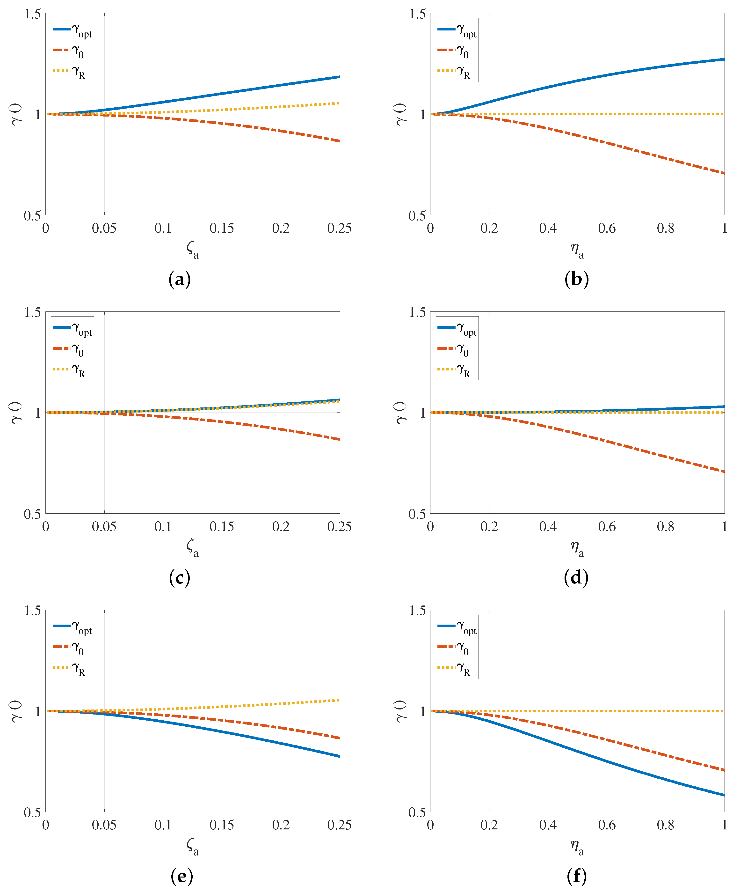
In Figure 4, the optimal tuning parameter ${\gamma }_{\mathrm{opt}}$ is compared to the quasi-optimal tuning parameter ${\gamma }_0$ and the approximated tuning parameter ${\gamma }_R$, highlighting their dependency on damping. Both ${\gamma }_{\mathrm{opt}}$ and ${\gamma }_0$ exhibit damping-dependent behaviour with distinct slopes, while ${\gamma }_R$ displays a minimal sensitivity to viscous damping and no dependence on structural damping. The maximum difference between the approximated and optimal tuning parameters occurs when tuning above the host resonance frequency in the presence of structural damping, reaching disparities of up to 40%. In contrast, the maximum difference between the quasi-optimal and optimal tuning parameters is observed when tuning below the resonance frequency, with potential deviations of up to 50% in the case of structural damping. Despite the larger differences associated with quasi-optimal tuning, its inherent simplicity and robustness in implementation [17,18] position it as the most viable choice for practical applications.

While the difference between ${\gamma }_{\mathrm{opt}}$ and ${\gamma }_0$ may be substantial in certain scenarios, the actual impact on the reduction D for these tuning values appears negligible in practical terms. In fact, as damping increases, the reduction function D becomes flatter. Figure 5 displays the difference in decibels between the reduction obtained with the quasi-optimal control algorithm and the optimal reduction levels, which consistently remains below 4 dB. In Figure 5b, the shaded area is due to numerical errors in evaluating the zeros of Equation (8). For small values of ${\zeta }_a$ and $\mathsf{\Omega }$, where the evaluation of ${\gamma }_{\mathrm{opt}}$ may fail, the optimal solution was approximated to ${\gamma }_{\mathrm{opt}}\approx 1$. In both cases, the reduction difference is small across the investigated range of damping and excitation frequencies, justifying the use of the quasi-optimal algorithm even for heavily damped structures.

6. Conclusions

This paper has presented a novel non-dimensional analysis of vibration neutralizers considering both structural and viscous damping. The objective was to provide a rigorous foundation that justifies a quasi-optimal tuning strategy that uses the cosine of the phase angle between the host structure and the neutralizer’s mass velocities as an error signal. A comparison between the proposed automatic quasi-optimal tuning algorithm and the optimal tuning approach has yielded insightful findings. The quasi-optimal algorithm demonstrates a remarkable accuracy in approximating the optimum tuning, particularly in scenarios characterized by low damping. Importantly, the analysis extends beyond theoretical considerations to practical engineering applications, revealing that the quasi-optimal algorithm remains effective even in the context of heavily damped structures.

References

- Bonello, P. Adaptive tuned vibration absorbers: Design principles, concepts and physical implementation. In Vibration Analysis and Control; Beltran-Carbajal, F., Ed.; IntechOpen: Rijeka, Croatia, 2011. [Google Scholar] [CrossRef]
- Franchek, M.A.; Ryan, M.W.; Bernhard, R.J. Adaptive passive vibration control. J. Sound Vib. 1996, 189, 565–585. [Google Scholar] [CrossRef]
- Bonello, P.; Groves, K.H. Vibration control using a beam-like adaptive tuned vibration absorber with an actuator-incorporated mass element. Proc. Inst. Mech. Eng. Part C J. Mech. Eng. Sci. 2009, 223, 1555–1567. [Google Scholar] [CrossRef]
- Kidner, M.R.F.; Brennan, M.J. Varying the Stiffness of a Beam-Like Neutralizer Under Fuzzy Logic Control. J. Vib. Acoust. 2001, 124, 90–99. [Google Scholar] [CrossRef]
- Walsh, P.L.; Lamancusa, J.S. A variable stiffness vibration absorber for minimization of transient vibrations. J. Sound Vib. 1992, 158, 195–211. [Google Scholar] [CrossRef]
- Rustighi, E.; Brennan, M.J.; Mace, B.R. A shape memory alloy adaptive tuned vibration absorber: Design and implementation. Smart Mater. Struct. 2004, 14, 19–28. [Google Scholar] [CrossRef]
- Williams, K.A.; Chiu, G.T.-C.; Bernhard, R.J. Dynamic modelling of a shape memory alloy adaptive tuned vibration absorber. J. Sound Vib. 2005, 280, 211–234. [Google Scholar] [CrossRef]
- Carneal, J.P.; Charette, F.; Fuller, C.R. Minimization of sound radiation from plates using adaptive tuned vibration absorbers. J. Sound Vib. 2004, 270, 781–792. [Google Scholar] [CrossRef]
- Bonello, P.; Brennan, M.J.; Elliott, S.J. Vibration control using an adaptive tuned vibration absorber with a variable curvature stiffness element. Smart Mater. Struct. 2005, 14, 1055–1065. [Google Scholar] [CrossRef]
- Brennan, M.J.; Bonello, P.; Rustighi, E.; Mace, B.R.; Elliott, S.J. Designs of a variable stiffness element for a tunable vibration absorber. In Proceedings of the ICA2004 (The 18th International Congress on Acoustics), Kyoto, Japan, 4–9 April 2004; Volume IV, pp. 2915–2918. [Google Scholar]
- Fosdick, R.; Ketema, Y. A thermoviscoelastic dynamic vibration absorber. J. Appl. Mech. 1998, 65, 17–24. [Google Scholar] [CrossRef]
- Rustighi, E.; Beaugrand, M. A viscoelastic adaptive tuned vibration absorber. In Proceedings of the MoViC2014: The 12th International Conference on Motion and Vibration, Sapporo, Japan, 3–7 August 2014; p. 10069. [Google Scholar]
- Wang, Y.; Li, L.; Hofmann, D.; Andrade, J.E.; Daraio, C. Structured fabrics with tunable mechanical properties. Nature 2021, 596, 238–243. [Google Scholar] [CrossRef] [PubMed]
- Rustighi, E.; Gardonio, P.; Cignolini, N.; Baldini, S.; Malacarne, C.; Perini, M. Vibration response of tuneable structured fabrics. In Proceedings of the ISMA2022 Including USD2022, Leuven, Belgium, 12–14 September 2022; pp. 2429–2439. [Google Scholar]
- Davis, C.L.; Lesieutre, G.A. An Actively Tuned Solid-State Vibration Absorber Using Capacitive Shunting of Piezoelectric Stiffness. J. Sound Vib. 2000, 232, 601–617. [Google Scholar] [CrossRef]
- Morgan, R.A.; Wang, K.W. Active-Passive Piezoelectric Absorbers for Systems Under Multiple Non-Stationary Harmonic Excitations. J. Sound Vib. 2002, 255, 685–700. [Google Scholar] [CrossRef]
- Rustighi, E.; Brennan, M.J.; Mace, B.R. Real-time control of a shape memory alloy adaptive tuned vibration absorber. Smart Mater. Struct. 2005, 14, 1184–1195. [Google Scholar] [CrossRef]
- Williams, K.A.; Chiu, G.T.-C.; Bernhard, R.J. Nonlinear control of a shape memory alloy adaptive tuned vibration absorber. J. Sound Vib. 2005, 288, 1131–1155. [Google Scholar] [CrossRef]
- Brennan, M.J. Vibration control using a tunable vibration neutralizer. Proc. Inst. Mech. Eng. Part C J. Mech. Eng. Sci. 1997, 211, 91–108. [Google Scholar] [CrossRef]
- Den Hartog, J.P. Mechanical Vibrations, 4th ed.; McGraw-Hill: New York, NY, USA, 1956. [Google Scholar]
Figure 1.
(a) A single-degree-of-freedom host structure with viscous damping; (b) an ATVN with viscous damping; (c) Host structure and ATVN with viscous damping; (d) Host structure and ATVN with hysteretic damping.
Figure 2.
Receptance of a single-degree-of-freedom host structure with viscous damping (continuous blue line) and receptance of the host structure with an ATVN tuned at the natural frequency of the host structure (continuous black line) and twenty percent below and above the natural frequency of the host structure (dotted and dashed black lines).
Figure 3.
Reduction levels D as function of with for viscous (a,c,e) and structural (b,d,f) damping: (a) and ; (b) and ; (c) and ; (d) and ; (e) and ; (f) and . The continuous black line shows the reduction levels obtained with the optimal tuning strategy. The dashed line presents the reduction levels obtained with quasi-optimal damping.
Figure 4.
Optimal, quasi-optimal, and approximated tuning as a function of the damping for viscous (a,c,e) and structural (b,d,f) damping (): (a) and ; (b) and ; (c) and ; (d) and ; (e) and ; (f) and .
Figure 5.
Difference between the reduction levels D obtained with the quasi-optimal and the optimal strategies expressed in dBs: (a) viscous damping with , ; (b) structural damping with , .
Disclaimer/Publisher’s Note: The statements, opinions and data contained in all publications are solely those of the individual author(s) and contributor(s) and not of MDPI and/or the editor(s). MDPI and/or the editor(s) disclaim responsibility for any injury to people or property resulting from any ideas, methods, instructions or products referred to in the content. |
© 2024 by the author. Licensee MDPI, Basel, Switzerland. This article is an open access article distributed under the terms and conditions of the Creative Commons Attribution (CC BY) license (https://creativecommons.org/licenses/by/4.0/).
Share and Cite
MDPI and ACS Style
Rustighi, E. Optimal and Quasi-Optimal Automatic Tuning of Vibration Neutralizers. Vibration 2024, 7, 362-373. https://doi.org/10.3390/vibration7020018
AMA Style
Rustighi E. Optimal and Quasi-Optimal Automatic Tuning of Vibration Neutralizers. Vibration. 2024; 7(2):362-373. https://doi.org/10.3390/vibration7020018
Chicago/Turabian StyleRustighi, Emiliano. 2024. "Optimal and Quasi-Optimal Automatic Tuning of Vibration Neutralizers" Vibration 7, no. 2: 362-373. https://doi.org/10.3390/vibration7020018