Kinetic Approach to Pair Production in Strong Fields—Two Lessons for Applications to Heavy-Ion Collisions

Abstract

The kinetic-equation approach to particle production in strong, time-dependent external fields is revisited and three limiting cases are discussed for different field patterns: the Sauter pulse, a harmonic pulse with a Gaussian envelope, and a Poisson-distributed stochastic field. It is shown that for transient subcritical electric fields $E\left(t\right)$ a finite residual particle number density $n(\infty )$ would be absent if the field-dependence of the dynamical phase in the Schwinger source term would be neglected. In this case the distribution function of created particles follows the law $f\left(t\right)\sim E^2\left(t\right)$. Two lessons for particle production in heavy-ion collisions are derived from this exercise. First: the shorter the (Sauter-type) pulse, the higher the residual density of produced particles. Second: although the Schwinger process in a string-type field produces a non-thermal particle spectrum, a Poissonian distribution of the (fluctuating) strings produces a thermal spectrum with an apparent temperature that coincides with the Hawking–Unruh temperature for the mean value of the string tension.

1. Introduction

The kinetic equation (KE) approach to particle production in strong, time-dependent external fields by the dynamical or dynamically assisted Schwinger mechanism (see, e.g., reference [1] for a recent review) has a broad spectrum of applications in different fields of Physics, ranging from high-intensity laser colliders to nuclear collisions and graphene in an external (laser) field. Even in the case when spatially homogeneous fields are considered the momentum distribution of the produced particles shows a complex pattern, reminding of interference fringes [2,3]. Therefore, it is instructive to consider limiting cases which may already provide valuable insights for phenomenological applications. In this spirit we shall consider in the present work the case of spatially homogeneous fields with three approximations to the Schwinger source term in the KE and three examples for the temporal pulse shape of the external field in order to draw conclusions for the systematics of particle production in relativistic heavy-ion collisions. Hereby we focus on the questions of how to maximize the yield of produced particles and how to explain their thermal-like spectra when they would be produced by a Schwinger mechanism.

This work is organized in the following way. In Section 2, the KE approach to particle production is shortly summarized, the differential form of the KE is given and three approximations are derived: the Markovian limit, the low-density approximation (LDA) and the low-field limit. In Section 3, the full solutions of the KE for two temporal pulse shapes are given (Sauter and Gaussian envelope harmonic (GEH) pulse) and compared with the results for the three approximations. In Section 4 and Section 5 the two lessons for the phenomenology of particle production in heavy-ion collisions are presented and in Section 6 we draw the conclusions.

2. Kinetic Approach to Particle Production

Our investigation is based on a KE which is a nonperturbative consequence of the fundamental equations of motion of QED. The KE for the (quasi-)particle distribution function can be derived from the Dirac equation by a canonical time-dependent Bogoliubov transformation [4]. This method is valid only in a spatially-uniform time-dependent field. In the case of a linearly polarized electric field with the vector potential $A^{\mu }\left(t\right)=(0,0,0,A\left(t\right))$ (Hamiltonian gauge) we obtain a non-Markovian integro-differential collisionless KE [5]

$$\frac{df(\overline{p},t)}{dt}=\frac{1}{2}\lambda (\overline{p},t){\int }_{t_0}^{t}d{t}^{\prime }\lambda (\overline{p},t^{\prime })\left[1-2f(\overline{p},t^{\prime })\right]cos\left(2[\mathsf{\Theta }(\overline{p},t)-\mathsf{\Theta }(\overline{p},t^{\prime })]\right),$$

(1)

where

$$\lambda (\overline{p},t)=\frac{eE\left(t\right){\epsilon }_{\perp }}{{\omega }^2(\overline{p},t)}$$

(2)

is the amplitude of vacuum transitions governing the rate of particle production. The dynamical phase,

$$\mathsf{\Theta }(\overline{p},t)={\int }_{t_0}^{t}d{t}^{\prime }\omega (\overline{p},t^{\prime }),$$

(3)

describes the vacuum oscillations (Zitterbewegung) with a frequency of the energy gap $2\omega (\overline{p},t)$ between lower ($\omega <-m$) and upper ($\omega >m$) continua (one can regard particle creation as an excitation of massive field quanta from lower to upper continua just like electrons and holes in the solid state physics models). Due to the fact that our calculations are performed in Hamiltonian gauge it is convenient to use a cylindrical system of coordinates, so it is natural to express the dispersion relation,

$$\omega (\overline{p},t)=\sqrt{{\epsilon }_{\perp }^2\left({\overline{p}}_{\perp }\right)+P^2({\overline{p}}_{\parallel },t)},$$

(4)

in terms of the transverse energy and the parallel canonical momentum,

$$\begin{array}{ccc}\hfill {\epsilon }_{\perp }\left({\overline{p}}_{\perp }\right)& =& \sqrt{m^2+{\overline{p}}_{\perp }^2},\hfill \end{array}$$

(5)

$$\begin{array}{ccc}\hfill P({\overline{p}}_{\parallel },t)& =& {\overline{p}}_{\parallel }-eA\left(t\right).\hfill \end{array}$$

(6)

Here m is the electron mass, e is the charge, ${\overline{p}}_{\perp }$ is the momentum component perpendicular to the field vector, whereas ${\overline{p}}_{\parallel }$ is the momentum component parallel to the field.

For the initial condition we choose

$$f(\overline{p},t){|}_{t=t_0}=0.$$

(7)

2.1. Differential Form

The numerical evaluation of the integro-differential Equation (1) through straightforward double time integration is highly ineffective. First of all, one needs to deal with the rapidly oscillating term $cos\left(2[\mathsf{\Theta }(\overline{p},t)-\mathsf{\Theta }(\overline{p},t^{\prime })]\right)$. To address this problem we can take the integration step small enough. Second, due to the non-Markovian character of the equation, it is required to store the whole pre-history of $f\left(t\right)$ in the computer memory. Luckily, one can avoid these complications by transforming (1) to a time local system of differential equations [6,7]. In order to perform the transformation we introduce two auxiliary functions

$$\begin{array}{ccc}\hfill u\left(t\right)& =& {\int }_{t_0}^{t}d{t}^{\prime }\lambda (\overline{p},t^{\prime })\left[1-2f(\overline{p},t^{\prime })\right]cos\left(2[\mathsf{\Theta }(\overline{p},t)-\mathsf{\Theta }(\overline{p},t^{\prime })]\right),\hfill \end{array}$$

(8)

$$\begin{array}{ccc}\hfill v\left(t\right)& =& {\int }_{t_0}^{t}d{t}^{\prime }\lambda (\overline{p},t^{\prime })\left[1-2f(\overline{p},t^{\prime })\right]sin\left(2[\mathsf{\Theta }(\overline{p},t)-\mathsf{\Theta }(\overline{p},t^{\prime })]\right).\hfill \end{array}$$

(9)

The auxiliary functions $u(\overline{p},t)$ and $v(\overline{p},t)$ describe vacuum polarization effects [8]. The differentiation of these functions with respect to t together with

$${\partial }_t\left([\mathsf{\Theta }(\overline{p},t)-\mathsf{\Theta }(\overline{p},t^{\prime })]\right)={\partial }_t{\int }_{t^{\prime }}^t\omega (\overline{p},t^{″})d{t}^{″}=\omega (\overline{p},t)$$

(10)

and Equation (1) leads to a coupled system of first order differential equations [7]

$$\begin{array}{ccc}\hfill \dot{f}& =& \frac{1}{2}\lambda (\overline{p},t)u\left(t\right),\hfill \end{array}$$

(11)

$$\begin{array}{ccc}\hfill \dot{u}& =& \lambda (\overline{p},t)\left[1-2f(\overline{p},t)\right]-2\omega (\overline{p},t)v\left(t\right),\hfill \end{array}$$

(12)

$$\begin{array}{ccc}\hfill \dot{v}& =& 2\omega (\overline{p},t)u\left(t\right),\hfill \end{array}$$

(13)

with the initial conditions

$$f\left(t_0\right)=u\left(t_0\right)=v\left(t_0\right)=0.$$

(14)

The above system of Equations (11)–(13) is much simpler to solve numerically.

2.2. Three Approximations to the Schwinger Source Term

In this section, we discuss three related approximations which can be obtained when the applied external electric field, $E\ll E_c$, is considerably smaller than the critical field strength [6,9].

$$E_c=\frac{m^2{c}^3}{e\hslash }\simeq 1.32\times {10}^{18}\mathrm{V}/\mathrm{m}.$$

(15)

The first approximation is the low density limit. When the electric field E is small we expect the probability of pair creation to be small $f(\overline{p},t)\ll 1$, hence $1-2f(\overline{p},t)\approx 1$. Consequently, the source term (r.h.s. of (1)) in LDA assumes the following form

$${\mathcal{S}}^{\mathrm{LDA}}\left(t\right)=\frac{1}{2}\lambda (\overline{p},t){\int }_{t_0}^{t}d{t}^{\prime }\lambda (\overline{p},t^{\prime })cos\left(2[\mathsf{\Theta }(\overline{p},t)-\mathsf{\Theta }(\overline{p},t^{\prime })]\right).$$

(16)

2.2.1. Markovian Limit

In the Markovian limit, one replaces the time argument $t^{\prime }$ in the statistical factor of (1) by the actual time t thus neglecting dependence on pre-history of the process [10],

$$\frac{d{f}^M\left(t\right)}{dt}=[1-2f^M\left(t\right)]{\mathcal{S}}^{\mathrm{LDA}}\left(t\right)={\mathcal{S}}^M\left(t\right).$$

(17)

Then, for the initial condition $f\left(t_0\right)=0$, the solution of (17) is given by

$$f^M\left(t\right)=\frac{1}{2}\left(1-exp\left[-2{\int }_{t_0}^{t}d{t}^{\prime }{\mathcal{S}}^{\mathrm{LDA}}\left(t^{\prime }\right)\right]\right).$$

(18)

2.2.2. Low-Density Approximation (LDA)

The expansion of $f^M$ in powers of the argument of the exponential function leads to

$$f^M\left(t\right)={\int }_{t_0}^{t}d{t}^{\prime }{\mathcal{S}}^{\mathrm{LDA}}\left(t^{\prime }\right)-{\left({\int }_{t_0}^{t}d{t}^{\prime }{\mathcal{S}}^{\mathrm{LDA}}\left(t^{\prime }\right)\right)}^2+\mathcal{O}\left[{\left({\int }_{t_0}^{t}d{t}^{\prime }{\mathcal{S}}^{\mathrm{LDA}}\left(t^{\prime }\right)\right)}^3\right].$$

(19)

Provided that the integral in (18) is small we can keep only the leading term and get the low-density solution

$$f^{\mathrm{LDA}}\left(t\right)={\int }_{t_0}^{t}d{t}^{\prime }{\mathcal{S}}^{\mathrm{LDA}}\left(t^{\prime }\right).$$

(20)

The low-density limit gives us a tool to demonstrate the positive definiteness of the distribution function. Using the trigonometric identity $cos(\alpha -\beta )=cos\alpha ·cos\beta +sin\alpha ·sin\beta$, we rewrite (20) as

$$\begin{array}{c}\hfill f^{\mathrm{LDA}}\left(t\right)=\frac{1}{2}\underset{t_0}{\overset{t}{\int }}d{t}^{\prime }{g}_1\left(t^{\prime }\right)\underset{t_0}{\overset{t^{\prime }}{\int }}d{t}^{″}{g}_1\left(t^{″}\right)+\frac{1}{2}\underset{t_0}{\overset{t}{\int }}d{t}^{\prime }{g}_2\left(t^{\prime }\right)\underset{t_0}{\overset{t^{\prime }}{\int }}d{t}^{″}{g}_2\left(t^{″}\right),\end{array}$$

(21)

$$g_{1,2}\left(\tau \right)=\lambda \left(\tau \right)\left\{\begin{array}{c}cos\left[2\mathsf{\Theta }\right(\tau \left)\right]\\ sin\left[2\mathsf{\Theta }\right(\tau \left)\right]\end{array}\right\}.$$

The application of the mathematical identity

$$\underset{t_0}{\overset{t}{\int }}d{t}^{\prime }A\left(t^{\prime }\right)\underset{t_0}{\overset{t^{\prime }}{\int }}d{t}^{″}B\left(t^{″}\right)=\frac{1}{2}\underset{t_0}{\overset{t}{\int }}d{t}^{\prime }A\left(t^{\prime }\right)\underset{t_0}{\overset{t}{\int }}d{t}^{″}B\left(t^{″}\right)$$

(22)

to (21) leads to the quadratic form

$$f^{\mathrm{LDA}}\left(t\right)=\frac{1}{4}{\left(\underset{t_0}{\overset{t}{\int }}d{t}^{\prime }{g}_1\left(t^{\prime }\right)\right)}^2+\frac{1}{4}{\left(\underset{t_0}{\overset{t}{\int }}d{t}^{\prime }{g}_2\left(t^{\prime }\right)\right)}^2.$$

(23)

Now it is straightforward to see that the distribution function in the LDA is positive definite as is required by the interpretation of the distribution function as a probability

$$f^{\mathrm{LDA}}\left(t\right)\ge 0.$$

(24)

2.2.3. Low-Field Limit

A further simplification of (23) can be obtained by expanding the dispersion relation with respect to a small external field $A\approx 0$,

$$\omega (\overline{p},t)=\sqrt{m^2+{\overline{p}}_{\perp }^2+{\overline{p}}_{\parallel }^2}-\frac{{\overline{p}}_{\parallel }eA}{\sqrt{m^2+{\overline{p}}_{\perp }^2+{\overline{p}}_{\parallel }^2}}+\mathcal{O}\left(A^2\right),$$

(25)

and keeping only the leading order by assuming the smallness of the vector potential

$$\omega (\overline{p},t)\approx \sqrt{m^2+{\overline{p}}_{\perp }^2+{\overline{p}}_{\parallel }^2}\equiv a.$$

(26)

Immediately one gets

$$\mathsf{\Theta }(\overline{p},t)={\int }_{t_0}^{t}d{t}^{\prime }\omega (\overline{p},t^{\prime })=a(t-t_0).$$

(27)

Then, we have to move out $\lambda$ in front of the integrals in (23),

$$\underset{t_0}{\overset{t}{\int }}d{t}^{\prime }{g}_1\left(t^{\prime }\right)=\lambda \left(t\right)\underset{t_0}{\overset{t}{\int }}d{t}^{\prime }cos\left[2a(t^{\prime }-t_0)\right]=\lambda \left(t\right)\frac{sin\left[2a(t-t_0)\right]}{2a},$$

(28)

$$\underset{t_0}{\overset{t}{\int }}d{t}^{\prime }{g}_1\left(t^{\prime }\right)=\lambda \left(t\right)\underset{t_0}{\overset{t}{\int }}d{t}^{\prime }sin\left[2a(t^{\prime }-t_0)\right]=-\lambda \left(t\right)\frac{cos\left[2a(t-t_0)\right]}{2a},$$

(29)

to obtain

$$f^0(\overline{p},t)={\lambda }^2\left(t\right)\frac{1}{16a^2}.$$

(30)

Applying a system of units such that $m=1$ leads to

$$f^0(\overline{p}=0,t)=\frac{E^2\left(t\right)}{16}.$$

(31)

3. Results for Sauter Pulse and Gaussian-Envelope Harmonic (GEH) Pulse

In this work we consider the simplest model of the external laser-like field, namely the linearly polarized, time-dependent and spatially homogeneous electric pulse. We solved the KE (1) numerically for the two field shapes. The first one, the so-called Sauter pulse [11] is defined by

$$A\left(t\right)=-E_0\tau tanh\frac{t}{\tau },E\left(t\right)=\frac{E_0}{{cosh}^2\frac{t}{\tau }},$$

(32)

with $\tau$ being the characteristic duration of action. The second one, called the GEH pulse, is given by

$$\begin{array}{ccc}\hfill E\left(t\right)& =& E_{0}cos(\omega t+\phi )exp(-\frac{t^2}{2{\tau }^2}),\hfill \end{array}$$

(33)

$$\begin{array}{ccc}\hfill A\left(t\right)& =& -\sqrt{\frac{\pi }{8}}{E}_0\tau exp(-\frac{1}{2}{\sigma }^2+i\phi )\times \mathrm{erf}\left(\frac{t}{\sqrt{2}\tau }-i\frac{\sigma }{\sqrt{2}}\right)+c.c.,\hfill \end{array}$$

(34)

where $\sigma =\omega \tau$ is a dimensionless measure for the characteristic duration of the pulse $\tau$ connected with the number of periods of the carrier field [12].

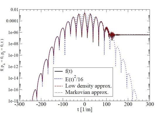
The impact of the above mentioned approximations on the fermionic distribution function for case of the Sauter have been presented on Figure 1. The analysis of these graphs shows:

• In case of a critical field strength $E_0\sim E_c$ and $t>0>t_0$ one gets $f^{\mathrm{LDA}}\left(t\right)>f^M\left(t\right)>f\left(t\right)$. This happens due to the presence of the factor $(1-2f)$ in (1) and its absence in (16).
• When $E_0\sim {10}^{-1}{E}_c$, the Markovian and the low-density approximation give similar values for the distribution functions so that $f^{\mathrm{LDA}}\left(t\right)\approx f^M\left(t\right)>f\left(t\right)$.
• In the case when $E_0\sim {10}^{-2}{E}_c$ we obtain $f^{\mathrm{LDA}}\left(t\right)\approx f^M\left(t\right)\approx f\left(t\right)$.
• When the external field is $E_0\sim {10}^{-2}{E}_c$, the distribution function is given by $f\left(t\right)\sim f^{\left(0\right)}\left(t\right)=E{\left(t\right)}^2$/16 at least for some finite period of time. For higher field strength, such an equality may not hold.
• When distribution function $f\left(t\right)$ follows the trend of $E{\left(t\right)}^2$/16 we are dealing with the quasi-particle electron-positron plasma (QEPP). However, when the distribution function reaches its asymptotic (residual) value $f\left(t\right)=const$, the state of the residual electron-positron plasma (REPP) is attained. In-between, there is a transition region characterized by fast oscillations which divides the system evolution into QEPP and REPP domains.
• For high field strengths, it is more difficult to distinguish the QEPP and REPP domains (see bottom panel of Figure 1).
• The higher the external field strength $E_0$, the faster $f\left(t\right)$ reaches the residual value.
• For shorter pulse duration the residual value $f(t\to \infty )$ is closer to maximal one.
• The approximation given by (31) assumes time-independence of the dispersion relation (26). In such circumstances $f\left(t\right)$ goes to zero when $E\left(t\right)\to 0$. No real particles are created, only virtual ones which disappear with the disappearance of the external electric field [7].

4. Lesson 1: Sauter Pulse Asymptotics

Now we are going to discuss the case of the Sauter pulse more in detail. We set $\overrightarrow{p}=0$ throughout. Its low-density approximation (LDA) [3] is denoted $f^{\mathrm{LDA}}$ and is given by

$$\begin{array}{ccc}\hfill f^{\mathrm{LDA}}\left(t\right)& =& \frac{1}{2}{\left|I\left(t\right)\right|}^2,I\left(t\right)=\underset{-\infty }{\overset{t}{\int }}d{t}^{\prime }J\left(t^{\prime }\right),\hfill \end{array}$$

(35)

$$\begin{array}{ccc}\hfill J\left(t\right)& =& \frac{eE\left(t\right)m}{m^2+e^{2}A{\left(t\right)}^2}{e}^{2i\mathsf{\Theta }\left(t\right)},\mathsf{\Theta }\left(t\right)=\underset{0}{\overset{t}{\int }}d{t}^{\prime }\sqrt{m^2+e^{2}A{\left(t\right)}^2}.\hfill \end{array}$$

(36)

Following Equations (35) and (32), it is easy to see that for $t\ll -\tau$

$$\begin{array}{ccc}\hfill A\left(t\right)& \sim & E_0\tau ,E\left(t\right)\sim 4E_0{e}^{2t/\tau },\mathsf{\Theta }\left(t\right)\sim \sqrt{m^2+{\left(e{E}_0\tau \right)}^2}t,\hfill \end{array}$$

(37)

$$\begin{array}{ccc}\hfill J\left(t\right)& \sim & \frac{4e{E}_{0}m}{m^2+{\left(e{E}_0\tau \right)}^2}{e}^{2t/\tau +2i\sqrt{m^2+{\left(e{E}_0\tau \right)}^2}t}.\hfill \end{array}$$

(38)

From these relations follows

$$I\left(t\right)\sim \frac{2e{E}_{0}m}{m^2+{\left(e{E}_0\tau \right)}^2}·\frac{e^{2t/\tau +2i\sqrt{m^2+{\left(e{E}_0\tau \right)}^2}t}}{1/\tau +i\sqrt{m^2+{\left(e{E}_0\tau \right)}^2}}=:I_{\mathrm{asy}}\left(t\right).$$

(39)

This allows us to define the small-t asymptotics of $f^{\mathrm{LDA}}$, denoted $f_{-\infty }$ as

$$\begin{array}{c}\hfill f_{-\infty }\left(t\right)=\frac{1}{2}{\left|I_{\mathrm{asy}}\left(t\right)\right|}^2=\frac{2{\left(e{E}_{0}m\right)}^2}{{\left[m^2+{\left(e{E}_0\tau \right)}^2\right]}^2\left[1/{\tau }^2+m^2+{\left(e{E}_0\tau \right)}^2\right]}{e}^{4t/\tau }.\end{array}$$

(40)

For $t\gg \tau$, we need the following symmetries

$$A(-t)=-A\left(t\right),E(-t)=E\left(t\right),\mathsf{\Theta }(-t)=-\mathsf{\Theta }\left(t\right),J(-t)=J{\left(t\right)}^{*}$$

(41)

and therefore

$$\begin{array}{ccc}\hfill I\left(t\right)& =& I(\infty )-\underset{t}{\overset{\infty }{\int }}d{t}^{\prime }J\left(t^{\prime }\right)=I(\infty )-\underset{-\infty }{\overset{-t}{\int }}d{t}^{\prime }J(-t^{\prime })=I(\infty )-\underset{-\infty }{\overset{-t}{\int }}d{t}^{\prime }J{\left(t^{\prime }\right)}^{*}=I(\infty )-I{(-t)}^{*}.\hfill \end{array}$$

(42)

The large-t asymptotic can thus be reduced to the small-t asymptotic and the constant $I(\infty )$. We denote it as $f_{\infty }$ and it is given by

$$\begin{array}{c}\hfill f_{\infty }\left(t\right)=\frac{1}{2}{\left|I(\infty )-I_{\mathrm{asy}}{(-t)}^{*}\right|}^2.\end{array}$$

(43)

In Figure 2 and Figure 3, we present the behavior of the Sauter pulse case together with the asymptotics introduced above. This comparison shows

• The shorter the Sauter-type pulse (smaller $\tau$), the higher the residual value of $f^{\mathrm{LDA}},f_{\infty }$ and f.
• The difference between the maximal value of f and its residual value grows with $\tau$. The same situation concerns $f^{\mathrm{LDA}}$. This feature is not observed in the case of $f_{\infty }$ and $f_{-\infty }$.
• Differences in the asymptotic values of $f^{\mathrm{LDA}}\left(t\right)$ and $f\left(t\right)$ grow with $E_0$ and with $\tau$.
• The curve $f_{\infty }$ exhibits a much weaker oscillatory behavior than f and $f^{\mathrm{LDA}}$.

The features of $f\left(t\right)$ can be useful in explaining phenomena related to heavy-ion collisions (HIC). Lorentz-contracted pancake-like nuclei at high energies are better sources for producing high parton densities than spherically-shaped nuclei at lower ones. This fact can be explained on the basis of Schwinger mechanism. After the collision of two ions, the color glass condensate (CGC) is likely formed, creating a strong longitudinal color electric field, called a flux tube. In this circumstance, the decay of the color electric field due to the Schwinger mechanism takes place. As shown in Figure 2 and Figure 3, particle creation is greatly enhanced when the external field duration is short. Then, the residual value of the distribution $f(t\to \infty )$ is higher and closer to the maximal value. Similarly, in HIC the number of created partons increases when nuclei collide rapidly.

Although the individual process of a particle-antiparticle pair creation leads to a non thermal spectrum, a statistical ensemble of the (fluctuating) color fields produces an apparently thermal spectrum with a temperature that is surprisingly given by the mean string tension in exactly the same functional form as the temperature of Hawking–Unruh radiation in a confining field. This observation can also be explained by the dynamical Schwinger mechanism.

Lesson 1: the shorter the Sauter-type pulse, the higher the residual density of produced particles. Therefore, Lorentz-contracted pancake-like nuclei at high energies are better sources for producing high parton densities than sphere-shaped nuclei at lower ones. Note, that we are speaking here not about the particle production in binary collisions, but rather by the vacuum decay in strong color-electric fields.

5. Lesson 2: Thermalization and Hawking Radiation

As an application of the Schwinger process the particle production in heavy-ion collisions has been considered which may proceed by the decay of color electric flux tubes [13,14,15,16]. The flux tubes are characterized by a linear, stringlike potential between color charges, analogous to the case of a homogeneous electric field considered by Schwinger. Using this analogy that $\left|eE\right|=\sigma$ with $\sigma \sim 0.19$ GeV${}^2$ being the string tension, the transverse energy spectrum of produced particles according to the Schwinger mechanism would be

$$\begin{array}{c}\hfill \frac{d{N}_{\mathrm{Schwinger}}}{d^2{p}_{\perp }}\sim exp\left(-\frac{\pi {\epsilon }_{\perp }^2}{\sigma }\right),\end{array}$$

(44)

with ${\epsilon }_{\perp }=\sqrt{m^2+p_{\perp }^2}$ being the transverse energy (5), often also denoted as “transverse mass” $m_{\perp }$. This spectrum of produced particles is Gaussian and thus would contradict the general observation of exponential particle spectra in heavy-ion collision experiments

$$\begin{array}{c}\hfill \frac{d{N}_{\exp }}{d^2{p}_{\perp }}\sim exp\left(-\frac{{\epsilon }_{\perp }}{T_{\mathrm{eff}}}\right),\end{array}$$

(45)

with an inverse slope parameter $T_{\mathrm{eff}}\sim 160$ MeV that can be considered as an effective temperature at the freeze-out (see, e.g., reference [17]). Thus the question arises how this transformation from a Gaussian to an exponential behavior of the spectrum (or the “thermalization”) could occur. It has been suggested that it proceeds via collisions described by a kinetic equation [18,19]. For a most recent discussion of the issue, see [20,21,22,23,24]. It has been questioned whether in high-energy nuclear collisions there is enough time for the thermal equilibration and the isotropization [25] of the system by collisions, after the particle production in a Schwinger process.

As an alternative picture for the emergence of a thermal particle spectrum in ultrarelativistic particle collisions the analogue of the Hawking–Unruh radiation has been discussed [26,27,28]. This reasoning predicts thermal spectra of hadrons with the Hawking–Unruh temperature

$$\begin{array}{c}\hfill T_H\left(\sigma \right)=\sqrt{\frac{\sigma }{2\pi }}\sim 173\mathrm{MeV},\end{array}$$

(46)

where for the string tension, $\sigma =1$ GeV/fm has been taken.

In this context it is interesting to note a possible synthesis of both pictures as provided by the argument elucidated by Bialas [29]. If the string tension in the Schwinger process for flux tube decay would fluctuate and follow, e.g., a Poissonian distribution

$$\begin{array}{c}\hfill P\left(\sigma \right)=exp(-\sigma /{\sigma }_0)/\sqrt{\pi \sigma {\sigma }_0},\end{array}$$

(47)

which is normalized $\int d\sigma P\left(\sigma \right)=1$ and has a mean value $\langle \sigma \rangle =\int d\sigma \sigma P\left(\sigma \right)={\sigma }_0/2$, then the initial Gaussian transverse energy spectrum (44) after averaging with the string tension fluctuations becomes exponential, i.e., thermal with the temperature parameter $T_{\mathrm{eff}}=\sqrt{\langle \sigma \rangle /\left(2\pi \right)}$,

$$\begin{array}{c}\hfill \int d\sigma P\left(\sigma \right)exp\left(-\frac{\pi {\epsilon }_{\perp }^2}{\sigma }\right)=exp\left(-\frac{{\epsilon }_{\perp }}{T}\right).\end{array}$$

(48)

Here the integral ${\int }_0^{\infty }dtexp[-t-k^2/\left(4t\right)]/\sqrt{\pi t}=exp(-k)$ has been used [30].

This coincides with the Hawking–Unruh picture of thermal hadron production, where in the case of fluctuating strings the string tension of Equation (46) is now replaced by its mean value. We would like to note at this point that a largely thermal spectrum would arise also from the solution of a kinetic equation with the Schwinger source term, as has been demonstrated by Florkowski in reference [31] for the case of parton creation (a more detailed calculation has recently been done in [20]). This demonstrates the dynamical origin of thermal spectra.

A recent study of the thermalization and isotropization question in the early stages of heavy-ion collisions [32] by solving a relativistic Boltzmann transport equation with a Schwinger source term for particle production from flux-tube decay goes beyond reference [20] by taking into account viscosity effects and $2\to 2$ collisions in the gluon sector. This study finds that for ideal fluid conditions with a minimal viscosity at the KSS bound $\eta =s/\left(4\pi \right)$ [33] already at a timescale below 1 fm/c the ratio of longitudinal to transverse pressure approaches unity with oscillations being damped out and the transverse momentum spectrum shows thermal behavior $dN/\left(p_T^{2}d{p}_{T}dy\right)\propto exp(-\beta p_T)$ with an inverse slope parameter fulfilling the ideal gas relationship ${\beta }^{-1}=T_{\mathrm{eff}}\propto {\epsilon }_{\mathrm{kin}}^{1/4}$, where ${\epsilon }_{\mathrm{kin}}$ is the kinetic energy density. It is interesting to note that this feature is reproduced by the much simpler model considered here which neglects collisions, spatial evolution and finite size as well as the backreaction of the produced particles on the field. It has, however, the advantage of being particularly suitable for discussing the temporal evolution (pulse shape) of the flux-tube field with special emphasis on subcritical field strengths (we remind that the account for confining boundary conditions in a flux tube of finite radial extension $r_0$ gives rise to an $r_0$-dependent suppression of the Schwinger pair production rate [34]).

In order to draw the link to the observed hadron spectra in heavy-ion collision experiments, it remains to consider also the hadronization process when starting from the parton level of description. For this purpose one could employ, e.g., kinetic theory approaches built on the basis of the Nambu–Jona–Lasinio model Lagrangian, see [35,36,37,38]. In this context, the dynamical chiral symmetry breaking in the quark sector plays an essential role as it triggers the binding of quarks into hadrons (inverse Mott effect). The increase in the sigma meson mass that accompanies the dynamical chiral symmetry breaking gives rise to additional sigma meson production by the inertial mechanism (see [39] and references therein). By the dominant decay $\sigma \to \pi \pi$ this leads to an additional population of low-momentum pion states and can contribute to the observed effect that s also discussed as a precursor of pion Bose condensation and may simultaneously resolve the Large Hadron Collider (LHC) proton puzzle [40] within a non-equilibrium model.

Lesson 2: although the individual Schwinger process of for creating a particle-antiparticle pair from flux-tube decay has a Gaussian transverse energy spectrum, a statistical distribution of the (fluctuating) color fields produces an apparently thermal (exponential) spectrum with an inverse slope parameter (effective temperature) $T_{\mathrm{eff}}=T_H\left(\langle \sigma \rangle \right)$ that surprisingly is given by the mean string tension in exactly the same functional form as the temperature of Hawking–Unruh radiation in a confining field.

6. Conclusions

In the present work, we have revisited the KE approach to particle production by the dynamical Schwinger effect. We have shown that in the case of subcritical external fields both, the LDA and the Markovian approximation to the source term give quite accurate estimations for the residual particle densities, to be observed after the field is switched off. It is an elucidating exercise to retain only the lowest order term in a low-field expansion of the dynamical phase of the Schwinger source term. In this case, the time-dependence of the distribution function of produced particles follows the temporal shape of the external field according to $f\left(t\right)\sim E^2\left(t\right)$ with the consequence that there are no produced particles in the final state where the field is absent. Thus the origin of particle production in subcritical fields can be traced to the self-interference (decoherence) of the virtual fields in the transient stage, formally accounted for by the time-dependent dynamical phase in the source term.

Two lessons for particle production in heavy-ion collisions are drawn from our exercise.

Lesson 1: The shorter the Sauter-type pulse, the higher the residual density of produced particles. Therefore, Lorentz-contracted pancake-nuclei at high energies are better sources for producing high parton densities than sphere-shaped nuclei at lower energies. Note, that in this argument we are considering only particle production from the vacuum decay in strong color fields as if particle production by collisions were absent.

Lesson 2: Although the individual Schwinger process of a particle-antiparticle pair has a non thermal (Gaussian) spectrum, a statistical distribution of the (fluctuating) color fields produces an apparently thermal (exponential) spectrum with a temperature (inverse slope parameter) that surprisingly is given by the mean string tension in exactly the same functional form as the temperature of Hawking–Unruh radiation in a confining field.

In a more complete kinetic description of particle production in a complex process like a heavy-ion collision, the subsequent stages following the creation of particles in the initial phase of the process should be included by adding elastic and inelastic scattering processes in the collision integrals of the system of kinetic equations for all relevant particle species. Thus, one can address the process of hadron production in heavy-ion collisions starting from parton production in strong field decay, their rescattering and conversion to hadrons (hadronization) with chemical equilibration and rescattering in the hadronic final state.

References

- Blaschke, D.B.; Smolyansky, S.A.; Panferov, A.; Juchnowski, L. Particle production in strong time-dependent fields. In Proceedings of the Quantum Field Theory at the Limits: From Strong Fields to Heavy Quarks (HQ 2016), Dubna, Russia, 18–30 July 2016; pp. 1–23. [Google Scholar] [CrossRef]
- Otto, A.; Seipt, D.; Blaschke, D.; Kämpfer, B.; Smolyansky, S.A. Lifting shell structures in the dynamically assisted Schwinger effect in periodic fields. Phys. Lett. B 2015, 740, 335–340. [Google Scholar] [CrossRef] [Green Version]
- Otto, A. The Dynamically Assisted Schwinger Process: Primary and Secondary Effects. Ph.D. Thesis, Technischen Universität Dresden, Dresden, Germany, 2017. [Google Scholar]
- Blaschke, D.B.; Prozorkevich, A.V.; Ropke, G.; Roberts, C.D.; Schmidt, S.M.; Shkirmanov, D.S.; Smolyansky, S.A. Dynamical Schwinger effect and high-intensity lasers. Realising nonperturbative QED. Eur. Phys. J. D 2009, 55, 341–358. [Google Scholar] [CrossRef] [Green Version]
- Blaschke, D.; Juchnowski, L.; Panferov, A.; Smolyansky, S. Dynamical Schwinger effect: Properties of the e+ e- plasma created from vacuum in strong laser fields. Phys. Part. Nucl. 2015, 46, 797–800. [Google Scholar] [CrossRef]
- Juchnowski, L. Quantum Kinetic Approach to Particle Production in Time Dependent External Fields. Ph.D. Thesis, University of Wroclaw, Wroclaw, Poland, 2018. in preparation. [Google Scholar]
- Bloch, J.C.R.; Mizerny, V.A.; Prozorkevich, A.V.; Roberts, C.D.; Schmidt, S.M.; Smolyansky, S.A.; Vinnik, D.V. Pair creation: Back reactions and damping. Phys. Rev. D 1999, 60, 116011. [Google Scholar] [CrossRef]
- Calzetta, E.A.; Hu, B.L.B. Nonequilibrium Quantum Field Theory; Cambridge University Press: Cambridge, UK, 2008. [Google Scholar]
- Schwinger, J.S. On gauge invariance and vacuum polarization. Phys. Rev. 1951, 82, 664–679. [Google Scholar] [CrossRef]
- Schmidt, S.M.; Blaschke, D.; Ropke, G.; Prozorkevich, A.V.; Smolyansky, S.A.; Toneev, V.D. NonMarkovian effects in strong field pair creation. Phys. Rev. D 1999, 59, 094005. [Google Scholar] [CrossRef]
- Sauter, F. Uber das verhalten eines elektrons im homogenen elektrischen feld nach der relativistischen theorie diracs. Z. Phys. 1931, 69, 742–764. [Google Scholar] [CrossRef]
- Panferov, A.D.; Smolyansky, S.A.; Otto, A.; Kämpfer, B.; Blaschke, D.B.; Juchnowski, L. Assisted dynamical Schwinger effect: Pair production in a pulsed bifrequent field. Eur. Phys. J. D 2016, 70, 56. [Google Scholar] [CrossRef]
- Casher, A.; Neuberger, H.; Nussinov, S. Chromoelectric flux tube model of particle production. Phys. Rev. D 1979, 20, 179–188. [Google Scholar] [CrossRef]
- Bialas, A.; Czyz, W. Chromoelectric flux tubes and the transverse momentum distribution in high-energy nucleus-nucleus collisions. Phys. Rev. D 1985, 31, 198. [Google Scholar] [CrossRef]
- Gatoff, G.; Kerman, A.K.; Matsui, T. The flux tube model for ultrarelativistic heavy ion collisions: Electrohydrodynamics of a quark gluon plasma. Phys. Rev. D 1987, 36, 114. [Google Scholar] [CrossRef]
- Braun, M.A.; Pajares, C. Particle production in nuclear collisions and string interactions. Phys. Lett. B 1992, 287, 154–158. [Google Scholar] [CrossRef]
- Broniowski, W.; Florkowski, W. Explanation of the RHIC p(T) spectra in a thermal model with expansion. Phys. Rev. Lett. 2001, 87, 272302. [Google Scholar] [CrossRef] [PubMed]
- Bialas, A.; Czyz, W. Boost invariant Boltzmann-vlasov equations for relativistic quark—Anti-quark plasma. Phys. Rev. D 1984, 30, 2371. [Google Scholar] [CrossRef]
- Kajantie, K.; Matsui, T. Decay of strong color electric field and thermalization in ultrarelativistic nucleus-nucleus collisions. Phys. Lett. B 1985, 164, 373–378. [Google Scholar] [CrossRef]
- Ryblewski, R.; Florkowski, W. Equilibration of anisotropic quark-gluon plasma produced by decays of color flux tubes. Phys. Rev. D 2013, 88, 034028. [Google Scholar] [CrossRef]
- Gelis, F.; Tanji, N. Schwinger mechanism revisited. Prog. Part. Nucl. Phys. 2016, 87, 1–49. [Google Scholar] [CrossRef] [Green Version]
- Gelis, F. Initial state and thermalization in the color glass condensate framework. In Quark-Gluon Plasma 5; Wang, X.N., Ed.; World Scientific: Singapore, 2016; pp. 67–129. [Google Scholar]
- Blaizot, J.P.; Liao, J.; Mehtar-Tani, Y. The thermalization of soft modes in non-expanding isotropic quark gluon plasmas. Nucl. Phys. A 2017, 961, 37–67. [Google Scholar] [CrossRef] [Green Version]
- Boguslavski, K.; Kurkela, A.; Lappi, T.; Peuron, J. Spectral function for overoccupied gluodynamics from real-time lattice simulations. Phys. Rev. D 2018, 98, 014006. [Google Scholar] [CrossRef]
- Attems, M.; Rebhan, A.; Strickland, M. Instabilities of an anisotropically expanding non-Abelian plasma: 3D + 3V discretized hard-loop simulations. Phys. Rev. D 2013, 87, 025010. [Google Scholar] [CrossRef]
- Castorina, P.; Kharzeev, D.; Satz, H. Thermal hadronization and Hawking–Unruh radiation in QCD. Eur. Phys. J. C 2007, 52, 187–201. [Google Scholar] [CrossRef] [Green Version]
- Castorina, P.; Satz, H. Hawking-Unruh hadronization and strangeness production in high energy collisions. Adv. High Energy Phys. 2014, 2014, 376982. [Google Scholar] [CrossRef]
- Castorina, P.; Iorio, A.; Satz, H. Hadron freeze-out and unruh radiation. Int. J. Mod. Phys. E 2015, 24, 1550056. [Google Scholar] [CrossRef]
- Bialas, A. Fluctuations of string tension and transverse mass distribution. Phys. Lett. B 1999, 466, 301–304. [Google Scholar] [CrossRef]
- Abramowitz, M.; Stegun, I. Handbook of Mathematical Functions; Dover: New York, NY, USA, 1964; p. 1026. [Google Scholar]
- Florkowski, W. Schwinger tunneling and thermal character of hadron spectra. Acta Phys. Polon. B 2004, 35, 799–808. [Google Scholar]
- Ruggieri, M.; Puglisi, A.; Oliva, L.; Plumari, S.; Scardina, F.; Greco, V. Modelling early stages of relativistic heavy ion collisions: Coupling relativistic transport theory to decaying color-electric flux tubes. Phys. Rev. C 2015, 92, 064904. [Google Scholar] [CrossRef]
- Kovtun, P.; Son, D.T.; Starinets, A.O. Viscosity in strongly interacting quantum field theories from black hole physics. Phys. Rev. Lett. 2005, 94, 111601. [Google Scholar] [CrossRef] [PubMed]
- Pavel, H.P.; Brink, D.M. q anti-q pair creation in a flux tube with confinement. Z. Phys. C 1991, 51, 119–125. [Google Scholar] [CrossRef]
- Rehberg, P.; Klevansky, S.P.; Hufner, J. Hadronization in the SU(3) Nambu-Jona-Lasinio model. Phys. Rev. C 1996, 53, 410–429. [Google Scholar] [CrossRef]
- Rehberg, P.; Bot, L.; Aichelin, J. Expansion and hadronization of a chirally symmetric quark—Meson plasma. Nucl. Phys. A 1999, 653, 415–435. [Google Scholar] [CrossRef]
- Friesen, A.V.; Kalinovsky, Y.V.; Toneev, V.D. Quark scattering off quarks and hadrons. Nucl. Phys. A 2014, 923, 1–18. [Google Scholar] [CrossRef] [Green Version]
- Marty, R.; Torres-Rincon, J.M.; Bratkovskaya, E.; Aichelin, J. Transport theory from the Nambu-Jona-Lasinio lagrangian. J. Phys. Conf. Ser. 2016, 668, 012001. [Google Scholar] [CrossRef]
- Juchnowski, L.; Blaschke, D.; Fischer, T.; Smolyansky, S.A. Nonequilibrium meson production in strong fields. J. Phys. Conf. Ser. 2016, 673, 012009. [Google Scholar] [CrossRef] [Green Version]
- Begun, V.; Florkowski, W.; Rybczynski, M. Explanation of hadron transverse-momentum spectra in heavy-ion collisions at = 2.76 TeV within chemical non-equilibrium statistical hadronization model. Phys. Rev. C 2014, 90, 014906. [Google Scholar] [CrossRef]
Figure 1.
Time evolution of the fermionic distribution function . Left panels: for the Sauter pulse (32) with . Right panels: for the Gaussian envelope harmonic (GEH) pulse (33) with , and nm. From the upper to the lower panel the electric field increases as . Time is scaled with the electron mass. Solid curve: full solution , dotted curve: /16, dashed curve: low density approximation given by (23), dot-dashed curve: Markovian limit given by (18).
Figure 2.
Time evolution of the fermionic distribution function in the case of Sauter pulse for . From the upper left to the lower right panel the pulse duration increases as . The solid curve is for the full solution . The dotted curve shows the low density approximation, the dashed curve depicts the small-t asymptotics , while the dot-dashed curve stands for the large-t asymptotics .
Figure 3.
Time evolution of the fermionic distribution function as in Figure 2, but for .
© 2019 by the authors. Licensee MDPI, Basel, Switzerland. This article is an open access article distributed under the terms and conditions of the Creative Commons Attribution (CC BY) license (http://creativecommons.org/licenses/by/4.0/).
Share and Cite
MDPI and ACS Style
Blaschke, D.B.; Juchnowski, L.; Otto, A. Kinetic Approach to Pair Production in Strong Fields—Two Lessons for Applications to Heavy-Ion Collisions. Particles 2019, 2, 166-179. https://doi.org/10.3390/particles2020012
AMA Style
Blaschke DB, Juchnowski L, Otto A. Kinetic Approach to Pair Production in Strong Fields—Two Lessons for Applications to Heavy-Ion Collisions. Particles. 2019; 2(2):166-179. https://doi.org/10.3390/particles2020012
Chicago/Turabian StyleBlaschke, David B., Lukasz Juchnowski, and Andreas Otto. 2019. "Kinetic Approach to Pair Production in Strong Fields—Two Lessons for Applications to Heavy-Ion Collisions" Particles 2, no. 2: 166-179. https://doi.org/10.3390/particles2020012