Anomaly-Induced Transport Phenomena from Imaginary-Time Formalism

Abstract

A derivation of anomaly-induced transport phenomena—the chiral magnetic/vortical effect—is revisited based on the imaginary-time formalism of quantum field theory. Considering the simplest anomalous system composed of a single Weyl fermion, we provide two derivations: perturbative (one-loop) evaluation of the anomalous transport coefficient, and the anomaly matching for the local thermodynamic functional.

1. Introduction

Quantum anomaly is one of the most fundamental properties of quantum systems, which keeps staying in the low-energy regime once it appears in an underlying UV theory [1,2]. As a consequence, the low-energy dynamics is strongly influenced by the existence of the quantum anomaly. A well-known example is the chiral anomaly in QCD, which gives rise to the Wess-Zumino term in the low-energy effective theory of QCD (the chiral perturbation theory) describing the neutral pion decay into two photons (${\pi }^0\to \gamma \gamma$) [3,4,5]. The notion of anomaly can be generalized to discrete symmetries of systems such as time-reversal symmetry. The anomaly matching argument [6,7] is actively applied to restrict the possible nontrivial ground states (See Refs. [8,9,10,11,12,13,14,15,16,17,18,19] for recent applications).

It has been recently noticed that quantum anomaly also appears even in the effective theory describing the real-time dynamics of nonequilibrium systems, e.g., hydrodynamics and the kinetic theory, and it affects the macroscopic transport properties in the hydrodynamic regime [20,21,22,23,24,25,26,27,28,29,30,31,32,33,34,35,36,37,38,39,40,41,42,43,44,45,46,47,48,49,50,51,52,53,54,55,56,57,58,59,60,61] (See also pioneering works by Vilenkin [62,63]). For example, the simplest anomalous system composed of a single right-handed Weyl fermion coupled to a background electromagnetic field shows interesting transport. When this system is put into an environment with a temperature T and a chemical potential ${\mu }_R$, the chiral anomaly induces the dissipationless current along the magnetic field $B^i$ given by

$${\langle {\widehat{J}}_R^i\rangle }_{\mathrm{ano}}={\sigma }_B{B}^i+{\sigma }_{\omega }{\omega }^i\mathrm{with}{\sigma }_B=\frac{{\mu }_R}{4{\pi }^2},{\sigma }_{\omega }=\frac{{\mu }_R^2}{4{\pi }^2}+\frac{T^2}{12},$$

(1)

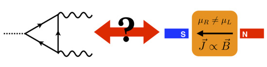
where ${\langle {\widehat{J}}_R^{\mu }\rangle }_{\mathrm{ano}}$ denotes the anomalous part of the expectation value of the right-handed current, and ${\sigma }_B$ (${\sigma }_{\omega }$) is regarded as the chiral magnetic (vortical) conductivity. The first and second terms in Equation (1) are called the chiral magnetic effect (CME) and chiral vortical effect (CVE), respectively (See Figure 1). It is worth pointing out that even in the weak coupling limit, ${\sigma }_B$ and ${\sigma }_{\omega }$ do not diverge unlike the usual conductivity because their existence is protected by the quantum anomaly.

These anomalous transports are believed to be universally present when the system under consideration contains the chiral anomaly. For example, they are expected to take place in the quark-gluon plasma created in high-energy heavy-ion collisions [64,65,66,67,68,69,70,71,72,73,74], astrophysical plasma including neutrino process [75,76,77,78,79,80], and Weyl semimetals realized in condensed matter physics [81,82,83,84,85,86,87,88,89,90]. While we have not observed clear experimental signal of the anomaly-induced transport in the first two systems, it has been recently reported that the experimental signals of the CME are achieved in the Weyl semimetal [91,92,93].

The theoretical derivation of the anomaly-induced transport phenomena has been remarkably developed in the past ten years, e.g., the direct field theoretical evaluation [20], the fluid/gravity correspondence [21,22,23,25], the phenomenological entropy-current analysis [24], the linear response theory [26,31,34,50,58], the kinetic theory [27,28,33,36,37,41,42,44,48,49,51,52,53,55,57,59,60,61], and the hydrostatic partition function method and extensions [29,30,32,35,38,39,40,43,45,46,54]. In this paper, we review the derivation of the anomaly-induced transport phenomena from the statistical mechanical viewpoint with the help of the imaginary-time (Matsubara) formalism of quantum field theory [94,95,96,97]. In particular, we demonstrate two derivations, which are basically on the same line as the last two derivations raised above. For that purpose, we consider the simplest anomalous system composed of a single Weyl fermion coupled to an external electromagnetic field. Although most results given in this paper has been already known, we give the clear rigorous justification of the hydrostatic partition function method for the anomalous system based on the statistical ensemble describing systems in general local thermal equilibrium. This shows that the hydrostatic partition function method is indeed not restricted to the real hydrostatic situation, but applicable to systems in general local thermal equilibrium.

The paper is organized as follows: In Section 2, we review the basic setup and formulation including the Zubarev’s nonequilibrium statistical operator methods [98,99,100] (See also Refs. [101,102,103,104] for a recent sophisticated revival of a similar idea). In Section 3, we then provide the perturbative evaluation of the chiral magnetic/vortical conductivity with the help of the (equilibrium) linear response theory, from which we can read off the constitutive relation for the anomalous current. In Section 4, we give another nonperturbative derivation based on the anomaly matching for the local thermodynamic functional. Section 5 is devoted to the summary and discussion.

2. Preliminaries for the Anomaly-Induced Transport Phenomena

In this section, we briefly summarize the formulation to derive the anomaly-induced transport phenomena based on the imaginary-time formalism [98,99,100,101,102,103,104].

2.1. Anomalous (Non-)Conservation Laws for a Single Weyl Fermion

Let us consider the system consisting of a right-handed Weyl fermions $\xi$ under an external $U\left(1\right)$ gauge field $A_{\mu }$ in a $(3+1)$ dimensional curved spacetime, whose action has the form:

$$\mathcal{S}[\xi ,{\xi }^{†};A_{\mu },e_{\mu }^a]=\int d^{4}xe\mathcal{L}\mathrm{with}\mathcal{L}\equiv \frac{i}{2}{\xi }^{†}\left(e_a^{\mu }{\sigma }^a{\overrightarrow{D}}_{\mu }-{\overleftarrow{D}}_{\mu }{\sigma }^a{e}_a^{\mu }\right)\xi ,e\equiv \det \left(e_{\mu }^a\right),$$

(2)

where we introduced ${\sigma }^a=(1,{\sigma }^i)$ with the Pauli matrices ${\sigma }^i(i=1,2,3)$. Here $e_{\mu }^a\left(e_a^{\mu }\right)$ denotes (inverse) vierbein satisfying $g_{\mu \nu }=e_{\mu }^a{e}_{\nu }^b{\eta }_{ab},{\eta }^{ab}=e_{\mu }^a{e}_{\nu }^b{g}^{\mu \nu }$ with the spacetime curved metric $g_{\mu \nu }$ and Minkowski metric ${\eta }_{ab}=\mathrm{diag}(-1,+1,+1,+1)$. The left and right covariant derivatives are defined as

$${\overrightarrow{D}}_{\mu }\xi \equiv {\partial }_{\mu }\xi -i({\mathcal{A}}_{\mu }+A_{\mu })\xi ,{\xi }^{†}{\overleftarrow{D}}_{\mu }\equiv {\partial }_{\mu }{\xi }^{†}+i{\xi }^{†}({\mathcal{A}}_{\mu }+A_{\mu })\mathrm{with}{\mathcal{A}}_{\mu }\equiv \frac{1}{2}{\omega }_{\mu }^{ab}{\mathsf{\Sigma }}_{ab},$$

(3)

where we introduced ${\mathsf{\Sigma }}_{ab}\equiv i({\sigma }^a{\overline{\sigma }}^b-{\sigma }^b{\overline{\sigma }}^a)/4$ with ${\overline{\sigma }}^a\equiv (-1,{\sigma }^i)$, which satisfies ${\sigma }^a{\overline{\sigma }}^b+{\sigma }^b{\overline{\sigma }}^a=2{\eta }^{ab}$. Furthermore, employing the torsionless condition, we can express the spin connection ${\omega }_{\mu }^{ab}=-{\omega }_{\mu }^{ba}$ as

$${\omega }_{\mu }^{ab}\equiv \frac{1}{2}{e}^{a\nu }{e}^{b\rho }(C_{\nu \rho \mu }-C_{\rho \nu \mu }-C_{\mu \nu \rho })\mathrm{with}{C}_{\mu \nu \rho }\equiv e_{\mu }^c({\partial }_{\nu }{e}_{\rho c}-{\partial }_{\rho }{e}_{\nu c}).$$

(4)

Although the classical action (2) is invariant under a set of infinitesimal diffeomorphisms, local Lorentz, and $U\left(1\right)$ gauge transformations with parameters $\chi \equiv \{{\zeta }^{\mu },{\alpha }_{ab},\theta \}$:

$$\left\{\begin{array}{c}{\delta }_{\chi }{e}_{\mu }^a={\zeta }^{\nu }{\nabla }_{\nu }{e}_{\mu }^a+e_{\nu }^a{\nabla }_{\mu }{\zeta }^{\nu }+{\alpha }_b^a{e}_{\mu }^b,\hfill \\ {\delta }_{\chi }{A}_{\mu }={\zeta }^{\nu }{\nabla }_{\nu }{A}_{\mu }+A_{\nu }{\nabla }_{\mu }{\zeta }^{\nu }+{\partial }_{\mu }\theta ,\hfill \\ {\delta }_{\chi }\xi ={\zeta }^{\nu }{\partial }_{\nu }\xi -{\displaystyle \frac{i}{2}}{\alpha }^{ab}{\mathsf{\Sigma }}_{ab}\xi +i\theta \xi ,\hfill \end{array}\right.$$

(5)

we encounter with the quantum anomaly attached to the Weyl fermion. As a consequence, the anomalous Ward-Takahashi identities results in the following operator identities corresponding to the (non-)conservation laws:

$$\left\{\begin{array}{c}{\nabla }_{\mu }{\widehat{T}}_{\nu }^{\mu }=F_{\nu \mu }{\widehat{J}}^{\mu },\hfill \\ {\nabla }_{\mu }{\widehat{J}}^{\mu }=-{\displaystyle \frac{1}{8}}C{\epsilon }^{\mu \nu \rho \sigma }{F}_{\mu \nu }{F}_{\rho \sigma }-\lambda {\epsilon }^{\mu \nu \rho \sigma }{R}_{\beta \mu \nu }^{\alpha }{R}_{\alpha \rho \sigma }^{\beta },\hfill \end{array}\right.$$

(6)

where we introduced the energy-momentum tensor ${\widehat{T}}_{\nu }^{\mu }$, $U\left(1\right)$ covariant charge current ${\widehat{J}}^{\mu }$ defined as

$$\begin{array}{cc}\hfill {\widehat{T}}^{\mu \nu }& =\frac{1}{e}\frac{\delta S}{\delta e_{\mu }^a}{e}_a^{\nu }=-\frac{i}{2}{\xi }^{†}({\sigma }^{\mu }\overrightarrow{D^{\nu }}-\overleftarrow{D^{\nu }}{\sigma }^{\mu })\xi +\frac{1}{4}{D}_{\rho }\left({\eta }^{†}\{{\sigma }^{\mu },{\mathsf{\Sigma }}^{\nu \rho }\}\eta \right)+\mathcal{L}{g}^{\mu \nu },\hfill \\ \hfill {\widehat{J}}^{\mu }& =\frac{1}{e}\frac{\delta S}{\delta e_{\mu }^a}={\xi }^{†}{\sigma }^{\mu }\xi .\hfill \end{array}$$

(7)

The Lorentz invariance implies that the antisymmetric part of the energy tensor vanishes: $T^{\mu \nu }+T^{\nu \mu }=0$; thus, $T^{\mu \nu }$ can be regarded as symmetric one. We also defined a field strength tensor for the background electromagnetic field $F_{\mu \nu }\equiv {\partial }_{\mu }{A}_{\nu }-{\partial }_{\nu }{A}_{\mu }$, and the Riemann curvature tensor $R_{\nu \rho \sigma }^{\mu }$ with the totally antisymmetric tensor ${\epsilon }^{\mu \nu \rho \sigma }$ satisfying ${\epsilon }^{0123}=1/e$. For notational simplicity, we drop the subscript R for the $U\left(1\right)$ current. Here $C=1/\left(4{\pi }^2\right)$ and $\lambda =1/\left(768{\pi }^2\right)$ denote the anomaly coefficients coming from gauge and gravitational sectors, respectively. Since $\lambda {\epsilon }^{\mu \nu \rho \sigma }{R}_{\beta \mu \nu }^{\alpha }{R}_{\alpha \rho \sigma }^{\beta }$ contains four derivatives, it does not contribute to the first-order hydrodynamics that we are interested in. Therefore, we will omit the gravitational part in the following discussion. Please note that while the gauge and diffeomorphism invariance provides two (non-)conservation laws, the local Lorentz invariance results in the symmetric property of the energy-momentum tensor operator. It is worth emphasizing that ${\widehat{J}}^{\mu }$ in Equation (6) is the covariant current which can be related to the consistent current ${\widehat{J}}_{\mathrm{con}}^{\mu }$ by

$${\widehat{J}}^{\mu }={\widehat{J}}_{\mathrm{con}}^{\mu }-\frac{1}{6}C{\epsilon }^{\mu \nu \rho \sigma }{A}_{\nu }{F}_{\rho \sigma }.$$

(8)

An analogue of this relation in local thermal equilibrium will appear in Section 4, and it plays an important role to see how the anomaly matching is realized for the local thermodynamic functional.

2.2. Zubarev’s Formula: Decomposing Dissipative and Nondissipative Transport

We then briefly review the Zubarev’s nonequilibrium statistical operator method from the modern viewpoint (See e.g., Refs. [98,99,100,101,102,103,104] for recent discussions) and specify from where the anomaly-induced transport arises. Assuming that the system is initially in local thermal equilibrium, the Zubarev’s formula provides us the expectation values of conserved current operators ${\widehat{\mathcal{J}}}_a^{\mu }\equiv \{{\widehat{T}}_{\nu }^{\mu },{\widehat{J}}^{\mu }\}$ over the initial density operator in the following compact form:

$$\langle {\widehat{\mathcal{J}}}_a^{\mu }(t,\mathit{x})\rangle ={\langle {\widehat{\mathcal{J}}}_a^{\mu }(t,\mathit{x})\rangle }_t^{\mathrm{LG}}+L_{ab}^{\mu \nu }(t,\mathit{x}){\nabla }_{\nu }{\lambda }^b(t,\mathit{x})+O\left({(\nabla \lambda )}^2\right),$$

(9)

where we introduced the intensive local thermodynamic parameters ${\lambda }^a\equiv \{{\beta }^{\mu },\nu \}$, which are related to the local fluid temperature $T=1/\beta$, four-velocity $u^{\mu }$, and the chemical potential $\mu$ through ${\beta }^{\mu }\equiv \beta u^{\mu },\nu \equiv \beta \mu$. We also defined the average over the local Gibbs distribution ${\widehat{\rho }}_{\mathrm{LG}}[\lambda ;t]$, which describes systems in local thermal equilibrium, for an arbitrary operator $\widehat{\mathcal{O}}$ as

$${\langle \widehat{\mathcal{O}}\rangle }_t^{\mathrm{LG}}\equiv \mathrm{Tr}\left({\widehat{\rho }}_{\mathrm{LG}}[\lambda ;t]\widehat{\mathcal{O}}\right)\mathrm{with}{\widehat{\rho }}_{\mathrm{LG}}[\lambda ;t]\equiv exp\left[-\widehat{S}[\lambda ;t]\right],\widehat{S}[\lambda ;t]=\widehat{K}[\lambda ;t]+\mathsf{\Psi }[\lambda ;t],$$

(10)

where the entropy operator $\widehat{S}[\lambda ;t]$ is composed of the part including operators ${\widehat{\mathcal{J}}}_a^{\mu }$ and normalization part for the density operator:

$$\begin{array}{cc}\hfill \widehat{K}[\lambda ;t]& \equiv -\int d{\mathsf{\Sigma }}_{t\mu }\left[{\beta }^{\nu }(t,\mathit{x}){\widehat{T}}_{\nu }^{\mu }(t,\mathit{x})+\nu (t,\mathit{x}){\widehat{J}}^{\mu }(t,\mathit{x})\right],\hfill \end{array}$$

(11)

$$\begin{array}{cc}\hfill \mathsf{\Psi }[\lambda ;t]& \equiv log\mathrm{Tr}exp\left[-\widehat{K}[\lambda ;t]\right].\hfill \end{array}$$

(12)

We here employed the fully covariant notion by introducing the constant time (spacelike) hypersurface defined by its perpendicular surface vector $d{\mathsf{\Sigma }}_{t\mu }\equiv -d^{3}x\sqrt{\gamma }{n}_{\mu }$. Choosing a certain globally defined time-coordinate function $\overline{t}\left(x\right)$, the unit normal vector $n_{\mu }$ can be expressed as

$$n_{\mu }\left(x\right)=-N\left(x\right){\partial }_{\mu }\overline{t}\left(x\right)\mathrm{with}N\left(x\right)\equiv {\left(-{\partial }^{\mu }\overline{t}\left(x\right){\partial }_{\mu }\overline{t}\left(x\right)\right)}^{-1/2},$$

(13)

where $N\left(x\right)$ is a so-called Lapse function. In addition, introducing the spatial coordinate on the $\overline{\mathit{x}}$, we have the induced metric ${\gamma }_{\mu \nu }=g_{\mu \nu }+n_{\mu }{n}_{\nu }$ whose spatial part gives $\gamma \equiv \det {\gamma }_{\overline{i}\overline{j}}$ (See e.g., Refs. [102,103] for a detailed geometric setup). The introduction of the covariantized notion looks a little bit complicated, but one can always take the flat limit by setting $\left(\overline{t}\left(x\right),\overline{\mathit{x}}\left(x\right)\right)=(t,\mathit{x})$, which results in e.g., $d{\mathsf{\Sigma }}_{t\mu }{|}_{\mathrm{flat}}=d^{3}x{\delta }_{\mu }^0$. Although it might be desirable to distinguish two coordinate systems defined by $(t,\mathit{x})$ and $(\overline{t},\overline{\mathit{x}})$, we will basically omit overline for the later one for notational simplicity since only $(\overline{t},\overline{\mathit{x}})$-coordinate system is mainly used. The normalization part $\mathsf{\Psi }[\lambda ;t]$ is the local thermodynamic functional called the Massieu-Planck functional, and plays a central role in Section 4.

The crucial point here is that by construction, we can identify the first term in the right-hand-side of Equation (9) as the nondissipative transport taking place in locally thermalized system, whereas the second term as the dissipative correction coming from the deviation from local thermal equilibrium. In other words, the formula (9) gives a way to decompose the non-dissipative and dissipative transport at least in the leading-order derivative expansion. The second term is proportional to the (local) thermodynamic forces ${\nabla }_{\nu }{\lambda }^b$, and coefficients in front of them are indeed specified as transport coefficients such as the bulk/shear viscosity, and conductivity. They are expressed by the two-point (Kubo) correlation function, which is nothing but the Green-Kubo formula for the transport coefficient [98,99,100,101,102,103,104]. On the other hand, nondissipative part is often assumed to be simply given by the usual constitutive relation for a perfect fluid. This is the case for parity-invariant systems, since the nondissipative derivative corrections are accompanied with higher-order derivatives for parity-invariant systems. Nevertheless, if we consider a system without parity symmetry—like the Weyl fermion system given in Equation (2)—we generally encounter with first-order nondissipative derivative corrections in ${\langle {\widehat{\mathcal{J}}}_a^{\mu }(t,\mathit{x})\rangle }_t^{\mathrm{LG}}$. This is the origin of the anomaly-induced transport, and we will focus on how we can evaluate ${\langle {\widehat{\mathcal{J}}}_a^{\mu }(t,\mathit{x})\rangle }_t^{\mathrm{LG}}$ in the remaining part of this paper.

Before closing this section, we put a short comment on the absence of the anomalous contribution to the entropy production. To see this, using the conservation laws (6), we express the entropy production operator $\widehat{\mathsf{\Sigma }}[t,t_0;\lambda ]\equiv \widehat{S}[\lambda ;t]-\widehat{S}[\lambda ;t_0]$ as

$$\widehat{\mathsf{\Sigma }}[t,t_0;\lambda ]={\int }_{t_0}^t{d}^{4}xe{\nabla }_{\mu }{\widehat{s}}^{\mu }\mathrm{with}{\nabla }_{\mu }{\widehat{s}}^{\mu }\equiv -\left({\nabla }_{\nu }{\beta }^{\mu }\right)\delta {{\widehat{T}}^{\mu }}_{\nu }-({\nabla }_{\mu }\nu +{\beta }^{\nu }{F}_{\mu \nu })\delta {\widehat{J}}^{\mu },$$

(14)

where we defined the local entropy production rate ${\nabla }_{\mu }{\widehat{s}}^{\mu }$ with $\delta \widehat{\mathcal{O}}\left(t\right)\equiv \widehat{\mathcal{O}}\left(t\right)-{\langle \widehat{\mathcal{O}}\left(t\right)\rangle }_t^{\mathrm{LG}}$. We thus find that the local equilibrium part of the constitutive relation ${\langle {\widehat{\mathcal{J}}}_a^{\mu }\rangle }_t^{\mathrm{LG}}$ which also contains the anomaly-induced transport as first-order derivative corrections, does not contribute to the local entropy production. This is perfectly consistent with the phenomenological derivation of the anomaly-induced transport based on the entropy-current analysis given in Ref. [24].

3. Perturbative Evaluation of Anomalous Transport Coefficients

In this section, we provide a simple perturbative derivation of the anomaly-induced transport given in Equation (1), and calculate anomalous transport coefficients ${\sigma }_B$ and ${\sigma }_{\omega }$ at the one-loop level.

3.1. Derivative Expansion of the Local Gibbs Distribution

First of all, we note that the local equilibrium part of the constitutive relation, or ${\langle {\widehat{\mathcal{J}}}_a^{\mu }(t,\mathit{x})\rangle }_t^{\mathrm{LG}}$, is a functional of local thermodynamic parameters ${\lambda }^a=\{{\beta }^{\mu },\nu \}$ and external fields $j\equiv \{A_{\mu },e_{\mu }^a\}$ at a fixed constant time t since the local Gibbs distribution ${\widehat{\rho }}_{\mathrm{LG}}[\lambda ;t]$ depends on the configuration of them. Thus, ${\langle {\widehat{\mathcal{J}}}_a^{\mu }(t,\mathit{x})\rangle }_t^{\mathrm{LG}}$ inherently contains the derivative correction coming from the local Gibbs distribution itself.

Suppose that our system is described by the local Gibbs distribution slightly deviated from the global equilibrium (Gibbs) distribution only with the magnetic field and fluid vorticity. We also turn off the external fields and take the flat limit. In that situation, approximating the fluid velocity and the magnetic field as

$$\left\{\begin{array}{c}{u}_j\left(x\right)=(x^i-x_0^i){\partial }_i{u}_j{|}_{x=x_0}=(x^i-x_0^i){ϵ}_{ijk}{\omega }^k,\hfill \\ A_j\left(x\right)=(x^i-x_0^i){\partial }_i{A}_j{|}_{x=x_0}={\displaystyle \frac{1}{2}}(x^i-x_0^i){ϵ}_{ijk}{B}^k,\hfill \end{array}\right.$$

(15)

we can expand the local Gibbs distribution on the top of the global Gibbs distribution as

$${\widehat{\rho }}_{\mathrm{LG}}[\lambda ;t]=\frac{1}{Z}{e}^{-\beta (\widehat{H}-\mu \widehat{N})}\left[1+T_{\tau }{\int }_0^{\beta }d\tau \mathsf{\Delta }\widehat{S}(t-i\tau )\right]\mathrm{with}\mathsf{\Delta }\widehat{S}\equiv \frac{1}{2}\int d^{3}x{ϵ}_{ijk}(x^i-x_0^i)\left({\widehat{J}}^j{B}^k+2{\widehat{T}}^{0j}{\omega }^k\right),$$

(16)

where we defined $\widehat{\mathcal{O}}(t-i\tau )\equiv e^{\tau (\widehat{H}-\mu \widehat{N})}\widehat{\mathcal{O}}\left(t\right)e^{-\tau (\widehat{H}-\mu \widehat{N})}$. Here $Z\equiv \mathrm{Tr}{e}^{-\beta (\widehat{H}-\mu \widehat{N})}$ denotes the partition function for the globally thermalized system, and we use ${\langle \widehat{\mathcal{O}}\rangle }_{\mathrm{eq}}\equiv \mathrm{Tr}\left(e^{-\beta (\widehat{H}-\mu \widehat{N})}\widehat{\mathcal{O}}\right)/Z$. Then, noting that the averaged current in global thermal equilibrium vanishes ${\langle {\widehat{J}}^i(t,{\mathit{x}}_0)\rangle }_{\mathrm{eq}}=0$, we can evaluate ${\langle {\widehat{J}}^i(t,{\mathit{x}}_0)\rangle }_t^{\mathrm{LG}}$ as

$$\begin{array}{cc}\hfill {\langle {\widehat{J}}^i(t,{\mathit{x}}_0)\rangle }_t^{\mathrm{LG}}& =\frac{1}{2}{\int }_0^{\beta }d\tau \int d^{3}x{ϵ}_{jkl}(x^j-x_0^j)\hfill \\ & \times \left[{\langle {\widehat{J}}^k(t-i\tau ,\mathit{x}){\widehat{J}}^i(t,{\mathit{x}}_0)\rangle }_{\mathrm{eq}}{B}^l(t,{\mathit{x}}_0)+2{\langle {\widehat{T}}^{0k}(t-i\tau ,\mathit{x}){\widehat{J}}^i(t,{\mathit{x}}_0)\rangle }_{\mathrm{eq}}{\omega }^l(t,{\mathit{x}}_0)\right]\hfill \\ & =\frac{i}{2}{ϵ}_{jkl}\left[{\partial }_{q_j}{\mathsf{\Delta }}_{J^k{J}^i}({\omega }_n,\mathit{q}){|}_{{\omega }_n=0,\mathit{q}=\mathbf{0}}{B}^l(t,{\mathit{x}}_0)+2{\partial }_{q_j}{\mathsf{\Delta }}_{T^{0k}{J}^i}({\omega }_n,\mathit{q}){|}_{{\omega }_n=0,\mathit{q}=\mathbf{0}}{\omega }^l(t,{\mathit{x}}_0)\right],\hfill \end{array}$$

(17)

where we performed the Fourier transformation to proceed the second line. It is now clear that we only need to evaluate two-point imaginary-time—not real-time—correlation functions, namely ${\langle {\widehat{J}}^k(t-i\tau ,\mathit{x}){\widehat{J}}^i(t,{\mathit{x}}_0)\rangle }_{\mathrm{eq}}$ and ${\langle {\widehat{T}}^{0k}(t-i\tau ,\mathit{x}){\widehat{J}}^i(t,{\mathit{x}}_0)\rangle }_{\mathrm{eq}}$, or their low-frequency and wave-number in the Fourier space.

3.2. One-loop Evaluation of Anomalous Transport Coefficients

We then evaluate the anomalous transport coefficients with the help of the Matsubara formalism. Since we expand the local Gibbs distribution on the top of global Gibbs distribution, the Euclidean action $S_E[\xi ,{\xi }^{†},\mu ]$ for the right-handed Weyl fermion is simply given by

$$S_E[\xi ,{\xi }^{†}]=-\sum _P{\xi }_a^{†}\left(P\right){\left({\mathcal{G}}_0^{-1}(\tilde{P})\right)}_{ab}{\xi }_b\left(P\right)\mathrm{with}{\mathcal{G}}_0^{-1}\left(P\right)\equiv {\sigma }^{\mu }{P}_{\mu },{\mathcal{G}}_0\left(P\right)=\frac{{\overline{\sigma }}^{\mu }{P}_{\mu }}{P^2},$$

(18)

where $a,b(=1,2)$ denote the spinor indices, and ${\mathcal{G}}_0\left(P\right)$ the free propagator for the Weyl fermion. We also defined ${\tilde{P}}_{\mu }\equiv \left(-i{\omega }_n-\mu ,\mathit{p})\right.$ with the Matsubara frequency ${\omega }_n\equiv (2n+1)\pi T$ and chemical potential $\mu$. As usual, we introduced the Fourier transformation

$$\xi (\tau ,\mathit{x})=T\sum _n\int \frac{d^3\mathit{p}}{{\left(2\pi \right)}^3}{e}^{-i{\omega }_n\tau +i\mathit{p}·\mathit{x}}\xi ({\omega }_n,\mathit{p}),$$

(19)

with the temperature $T\equiv 1/\beta$. Please note that the argument of the propagator in Equation (18) is not P but $\tilde{P}$, and, thus, it represents the propagator fully dressed by the chemical potential $\mu$. By using these, we need to evaluate the following diagrams:

(20)

where we will take the long-wave-length limit $Q\sim 0$.

First, let us evaluate the two-point current-current correlation function given by

(21)

where we used the free propagator defined in Equation (18). Here “$\mathrm{tr}$” denotes the trace over the spinor indices. With the help of the trace formula for the Pauli matrices

$$\mathrm{tr}{\overline{\sigma }}^{\mu }{\sigma }^{\nu }{\overline{\sigma }}^{\alpha }{\sigma }^{\beta }=-2i{\epsilon }^{\mu \nu \alpha \beta }+2{\eta }^{\mu \nu }{\eta }^{\alpha \beta }-2{\eta }^{\mu \alpha }{\eta }^{\nu \beta }+2{\eta }^{\mu \beta }{\eta }^{\nu \alpha },$$

(22)

we can decompose the two-point functions into the antisymmetric part and other parts. Since we are interested in the anomalous term which results from the antisymmetric part, we only focus on that part:

(23)

Next, let us evaluate the two-point momentum-current correlation function. Then, the same calculus brings about the following result

Putting these results all together, Equation (17) results in

$${\langle {\widehat{J}}^i(t,{\mathit{x}}_0)\rangle }_t^{\mathrm{LG}}=\frac{\mu }{4{\pi }^2}{B}^i(t,{\mathit{x}}_0)+\left(\frac{{\mu }^2}{4{\pi }^2}+\frac{T^2}{12}\right){\omega }^i(t,{\mathit{x}}_0),$$

(24)

which is nothing but Equation (1). To summarize the above analysis, we have derived the anomaly-induced transport—chiral magnetic/vortical effect—for the Weyl fermion by expanding the local Gibbs distribution. This clearly shows that information on the anomaly-induced transport is fully contained in ${\langle {\widehat{\mathcal{J}}}_a^{\mu }(t,\mathit{x})\rangle }_t^{\mathrm{LG}}$. Although we performed the direct expansion of the local Gibbs distribution in this section, there is another way to systematically evaluate ${\langle {\widehat{\mathcal{J}}}_a^{\mu }(t,\mathit{x})\rangle }_t^{\mathrm{LG}}$ as we will see in the next section.

4. Anomaly Matching for Local Thermodynamic Functional

In the previous section, we have explicitly shown that the local equilibrium part of constitutive relations ${\langle {\widehat{\mathcal{J}}}_a^{\mu }(t,\mathit{x})\rangle }_t^{\mathrm{LG}}$ indeed contains the information on the anomaly-induced transport. Although it is the one-loop perturbative calculation, we expect the result, or the value of anomalous transport coefficients, is protected by the underlying chiral anomaly, and remain the same even if we take into account the effect of interactions nonperturbatively. In this section, we provide another way to see the anomaly-induced transport putting the emphasis on the nonperturbative aspect of the anomaly. The key quantity is the local thermodynamic functional $\mathsf{\Psi }[\lambda ,j;t]$ already defined in Equation (12).

4.1. Basic Properties of Local Thermodynamic Functional

We here summarize basic properties of the Massieu-Planck functional $\mathsf{\Psi }[\lambda ,j;t]$: the exact path-integral expression of $\mathsf{\Psi }[\lambda ,j;t]$ and resulting symmetry properties together with the variational formula.

4.1.1. Path-Integral Formula and Resulting Symmetry

We will first summarize the key result for the Massieu-Planck functional (See Refs. [102,103] for the derivation). Using the energy-momentum tensor operator ${\widehat{T}}_{\nu }^{\mu }$ and covariant current operator ${\widehat{J}}^{\mu }$ resulting from (2), we can express the Massieu-Planck functional by the imaginary-time path-integral in the same way with the usual Matsubara formalism for global thermal equilibrium. After a little bit tedious calculation (See Ref. [103]), we eventually obtain

$$\mathsf{\Psi }[\lambda ,j;t]=\int \mathcal{D}\xi \mathcal{D}{\xi }^{†}exp\left(\tilde{\mathcal{S}}[\xi ,{\xi }^{†};\tilde{A},\tilde{e}]\right),$$

(25)

with the manifestly covariant action $\tilde{\mathcal{S}}[\xi ,{\xi }^{†};{\tilde{A}}_{\mu },{\tilde{e}}_{\mu }^a]$ given by

$$\tilde{\mathcal{S}}[\xi ,{\xi }^{†};{\tilde{A}}_{\mu },{\tilde{e}}_{\mu }^a]={\int }_0^{{\beta }_0}d\tau d^{3}x\tilde{e}\left[\frac{i}{2}{\xi }^{†}\left({\tilde{e}}_a^{\mu }{\sigma }^a{\overrightarrow{\tilde{D}}}_{\mu }-{\overleftarrow{\tilde{D}}}_{\mu }{\sigma }^a{\tilde{e}}_a^{\mu }\right)\xi \right]\mathrm{with}\tilde{e}\equiv \det \left({\tilde{e}}_{\mu }^a\right).$$

(26)

Here we introduced the thermal (inverse) vierbein ${\tilde{e}}_{\mu }^a\left({\tilde{e}}_a^{\mu }\right)$ and the external $U\left(1\right)$ gauge field ${\tilde{A}}_{\mu }$ in thermally emergent curved spacetime as

$${\tilde{e}}_0^a=e^{\sigma }{u}^a,{\tilde{e}}_i^a=e_i^a\mathrm{and}{\tilde{A}}_0=e^{\sigma }\mu ,{\tilde{A}}_i=A_i,$$

(27)

where recalling ${\beta }^{\mu }\left(x\right)\equiv \beta \left(x\right)u^{\mu }\left(x\right)$ and $\nu \left(x\right)=\beta \left(x\right)\mu \left(x\right)$, we used

$$e^{\sigma \left(x\right)}\equiv \beta \left(x\right)/{\beta }_0,\mu \left(x\right)\equiv \nu \left(x\right)/\beta \left(x\right),\beta \left(x\right)\equiv \sqrt{-g_{\mu \nu }\left(x\right){\beta }^{\mu }\left(x\right){\beta }^{\nu }\left(x\right)},$$

(28)

with a constant reference inverse temperature ${\beta }_0$. We also introduced $\tilde{e}\equiv det{\tilde{e}}_{\mu }^a$ and the covariant derivative in thermal spacetime as

$$\left\{\begin{array}{c}{\overrightarrow{\tilde{D}}}_{\mu }\xi \equiv {\tilde{\partial }}_{\mu }\xi -i({\tilde{\mathcal{A}}}_{\mu }+{\tilde{A}}_{\mu })\xi ,\hfill \\ {\xi }^{†}{\overleftarrow{\tilde{D}}}_{\mu }\equiv {\tilde{\partial }}_{\mu }{\xi }^{†}+i{\xi }^{†}({\tilde{\mathcal{A}}}_{\mu }+{\tilde{A}}_{\mu }),\hfill \end{array}\right.\mathrm{with}{\tilde{\partial }}_{\mu }\equiv (i{\partial }_{\tau },{\partial }_i),{\tilde{\mathcal{A}}}_{\mu }\equiv \frac{1}{2}{\tilde{\omega }}_{\mu }^{ab}{\mathsf{\Sigma }}_{ab},$$

(29)

where the thermal spin connection is expressed by the thermal vierbein ${\tilde{e}}_{\mu }^a$ through the same relation in the original spacetime (4).

As is shown in these, we can say that the Massieu-Planck functional is expressed as the path-integral in the presence of the emergent background curved spacetime and $U\left(1\right)$ gauge field. Figure 2 shows a schematic picture to compare the imaginary-time formalism in global and local thermal equilibrium.

Please note that this background structure is completely determined by configurations of the local thermodynamic variables ${\lambda }^a$ (and external fields j) on the constant time hypersurface in the original spacetime. The crucial point here is that all these quantities do not depend on the imaginary-time coordinate $\tau$, which leads to the Kaluza-Klein gauge symmetry. To see this clearly, we express the line element $d{\tilde{s}}^2\equiv {\tilde{e}}_{\mu }^a{\tilde{e}}_{\nu }^b{\eta }_{ab}d{\tilde{x}}^{\mu }\otimes d{\tilde{x}}^{\nu }$ and $U\left(1\right)$ gauge connection $\tilde{A}\equiv {\tilde{A}}_{\mu }d{\tilde{x}}^{\mu }$ in thermal spacetime as

$$\begin{array}{cc}\hfill d{\tilde{s}}^2& =-e^{2\sigma }{(d\tilde{t}+a_{i}d{x}^i)}^2+{\gamma }_{ij}^{\prime }d{x}^{i}d{x}^j,\hfill \end{array}$$

(30)

$$\begin{array}{cc}\hfill \tilde{A}& ={\tilde{A}}_0(d\tilde{t}+a_{i}d{x}^i)+{\tilde{A}}_i^{\prime }d{x}^i,\hfill \end{array}$$

(31)

with $d\tilde{t}\equiv -id\tau$. Here we defined the following quantities

$$a_i\equiv -e^{-\sigma }{u}_i,{\gamma }_{ij}^{\prime }\equiv {\gamma }_{ij}+e^{2\sigma }{a}_i{a}_j,{\tilde{A}}_i^{\prime }\equiv ={\tilde{A}}_i-{\tilde{A}}_0{a}_i.$$

(32)

Then, in addition to the spatial diffeomorphism invariance—invariance under spatial coordinate transformation $\mathit{x}\to {\mathit{x}}^{\prime }\left(\mathit{x}\right)$— we now see the background (30) and (31) is invariant under the transformation given by

$$\left\{\begin{array}{c}\tilde{t}\to \tilde{t}+\chi \left(\mathit{x}\right),\hfill \\ \mathit{x}\to \mathit{x},\hfill \\ a_i\left(\mathit{x}\right)\to a_i\left(\mathit{x}\right)-{\partial }_i\chi \left(\mathit{x}\right).\hfill \end{array}\right.$$

(33)

This is nothing but Kaluza-Klein gauge transformation, and $a_i$ is identified as the Kaluza-Klein gauge field. Please note that ${\gamma }_{ij}$ and ${\tilde{A}}_i=A_i$ do transform under the Kaluza-Klein gauge transformation so that ${\gamma }_{ij}^{\prime }$ and ${\tilde{A}}_i^{\prime }$ do not. Therefore, it is useful to employ Kaluza-Klein gauge invariant quantities ${\gamma }_{ij}^{\prime }$ and ${\tilde{A}}_i^{\prime }$ rather than ${\gamma }_{ij}$ and ${\tilde{A}}_i$ as basic building blocks to construct the Massieu-Planck functional. Furthermore, since the system is composed of the Weyl fermion, the apparent $U\left(1\right)$ gauge invariance for ${\tilde{A}}_i^{\prime }$ is anomalously broken. These spatial diffeomorphism, Kaluza-Klein gauge, and anomalous $U\left(1\right)$ gauge symmetries provide a basic restriction to the Massieu-Planck functional.

4.1.2. Variational Formula in the Presence of Quantum Anomaly

We then provide the variational formula for the Massieu-Planck functional $\mathsf{\Psi }[\lambda ,j;t]$, and show all information on ${\langle {\widehat{\mathcal{J}}}_a^{\mu }(t,\mathit{x})\rangle }_t^{\mathrm{LG}}$ is fully installed in it. To show this, let us consider the variation of $\widehat{K}$ defined in Equation (11) under the infinitesimal general coordinate and gauge transformation with a set of parameters ${\zeta }^{\mu }=ϵ{\beta }^{\mu }$ and $\theta =ϵ(\nu -\beta ·A)$. ($ϵ$ denotes an infinitesimal constant.) As a result, of the combination of diffeomorphism and $U\left(1\right)$ gauge transformations, the variation of the background $U\left(1\right)$ gauge field ${\delta }_{\lambda }{A}_{\mu }$ has the simple expression:

$${\delta }_{\lambda }{A}_{\mu }={\pounds }_{\beta }{A}_{\mu }+{\nabla }_{\mu }(\nu -\beta ·A)={\nabla }_{\mu }\nu +{\beta }^{\nu }{F}_{\nu \mu }.$$

(34)

The crucial point here is that $\widehat{K}$ remains invariant under the simultaneous transformation acting on both operators and external fields: ${\delta }_{\lambda }\widehat{K}\equiv {\delta }_{\lambda }^{\mathrm{para}}\widehat{K}+{\delta }_{\lambda }^{\mathrm{ope}}\widehat{K}=0$. This invariance can be shown by recalling all operators in $\widehat{K}$ are $U\left(1\right)$ gauge invariant, and, furthermore, rewriting $\widehat{K}$ as

$$\widehat{K}[t,{\lambda }^a,e_{\mu }^a,A_{\mu }]=\int d^{4}x\sqrt{\gamma }\delta (t-t\left(x\right))n_{\mu }\left(x\right){\lambda }^a\left(x\right){\widehat{\mathcal{J}}}_a^{\mu }\left(x\right),$$

(35)

from which we can clearly see diffeomorphism (reparameterization) invariance. Moreover, ${\delta }_{\lambda }^{\mathrm{ope}}\widehat{K}$ will also trivially vanish just because ${\delta }_{\lambda }^{\mathrm{ope}}\widehat{K}=[i\widehat{K},\widehat{K}]=0$. As a result, we have the operator identity ${\delta }_{\lambda }^{\mathrm{para}}\widehat{K}=0$.

Then, let us investigate ${\delta }_{\lambda }^{\mathrm{para}}\widehat{K}$ in detail, whose explicit definition is given by

$${\delta }_{\lambda }^{\mathrm{para}}\widehat{K}\equiv \int d^{4}x\left[\frac{\delta \widehat{K}}{\delta t\left(x\right)}{\pounds }_{\beta }t\left(x\right)+\frac{\delta \widehat{K}}{\delta {\lambda }^a\left(x\right)}{\pounds }_{\beta }{\lambda }^a\left(x\right)+\frac{\delta \widehat{K}}{\delta e_{\mu }^a\left(x\right)}{\pounds }_{\beta }{e}_{\mu }^a\left(x\right)+\frac{\delta \widehat{K}}{\delta A_{\mu }\left(x\right)}{\delta }_{\lambda }{A}_{\mu }\left(x\right)\right].$$

(36)

To rewrite the first term of this equation, noting $\delta (t-t\left(x\right))n_{\mu }=-N\delta (t-t\left(x\right)){\partial }_{\mu }t=N{\partial }_{\mu }\theta (t-t\left(x\right))$ following from the definition of $n_{\mu }$, and performing the integration by parts, we rewrite $\widehat{K}$ in Equation (35) as

$$\begin{array}{cc}\hfill \widehat{K}[t,{\lambda }^a,e_{\mu }^a,A_{\mu }]& =-\int d^{4}xe\theta (t-t\left(x\right)){\nabla }_{\mu }\left({\lambda }^a\left(x\right){\widehat{\mathcal{J}}}_a^{\mu }\left(x\right)\right)\hfill \\ & =-\int d^{4}xe\theta (t-t\left(x\right))\left({\widehat{T}}_{\nu }^{\mu }{\nabla }_{\mu }{\beta }^{\nu }+{\widehat{J}}^{\mu }({\nabla }_{\mu }\nu +{\beta }^{\nu }{F}_{\nu \mu })-\frac{1}{8}C\nu {\epsilon }^{\mu \nu \rho \sigma }{F}_{\mu \nu }{F}_{\rho \sigma }\right),\hfill \end{array}$$

(37)

where we used $e=N\sqrt{\gamma }$ and employed the operator identity for current operators (6) to proceed the second line. With the help of Equation (34) together with ${\nabla }_{\mu }{\beta }^{\nu }=e_a^{\nu }{\pounds }_{\beta }{e}_{\mu }^a+{\beta }^{\rho }{\omega }_{\rho \mu }^{\nu }$ followed from the so-called (torsionless) tetrad postulate ${\nabla }_{\mu }{e}_{\nu }^a+{\omega }_{\mu b}^a{e}_{\nu }^b=0$, Equation (37) enables us to obtain

$$\int d^{4}x\frac{\delta \widehat{K}}{\delta t\left(x\right)}{\pounds }_{\beta }t\left(x\right)=\int d^{4}x\sqrt{\gamma }\delta (t-t\left(x\right))\left[{\widehat{T}}_a^{\mu }{\pounds }_{\beta }{e}_{\mu }^a+{\widehat{J}}^{\mu }{\delta }_{\lambda }{A}_{\mu }-\frac{1}{8}C\nu {\epsilon }^{\mu \nu \rho \sigma }{F}_{\mu \nu }{F}_{\rho \sigma }\right]{\beta }^{\prime },$$

(38)

where we defined ${\beta }^{\prime }\equiv -{\beta }^{\mu }{n}_{\mu }$ and used the operator identity ${\widehat{T}}^{ab}-{\widehat{T}}^{ba}=0$. By using the identity

$$n_{\alpha }{\epsilon }^{\mu \nu \rho \sigma }{F}_{\mu \nu }{F}_{\rho \sigma }=-4{\epsilon }^{\mu \nu \rho \sigma }{n}_{\nu }{F}_{\rho \sigma }{F}_{\alpha \mu }.$$

(39)

the last term in the second line of Equation (38) can be further simplified as

$$\begin{array}{cc}\hfill \int d^{4}x\sqrt{\gamma }\delta (t-t\left(x\right))\left[\frac{1}{8}C\nu {\beta }^{\alpha }{n}_{\alpha }{\epsilon }^{\mu \nu \rho \sigma }{F}_{\mu \nu }{F}_{\rho \sigma }\right]& =-\int d^{4}x\sqrt{\gamma }\delta (t-t\left(x\right))\left[\frac{1}{2}C\nu {\beta }^{\alpha }{n}_{\nu }{\epsilon }^{\mu \nu \rho \sigma }{F}_{\rho \sigma }{F}_{\alpha \mu }\right]\hfill \\ & =-\int d^{4}x\sqrt{\gamma }\delta (t-t\left(x\right))C\nu B^{\mu }{\delta }_{\lambda }{A}_{\mu }.\hfill \end{array}$$

(40)

Here we defined the four-magnetic field as $B^{\mu }\equiv {\tilde{F}}^{\mu \nu }{n}_{\nu }={\epsilon }^{\mu \nu \rho \sigma }{n}_{\nu }{F}_{\rho \sigma }/2$, and neglected the surface term accompanied by the integration by parts. We thus obtain the following compact result:

$$\int d^{4}x\frac{\delta \widehat{K}}{\delta t\left(x\right)}{\pounds }_{\beta }t\left(x\right)=\int d^{4}x{\beta }^{\prime }\sqrt{\gamma }\delta (t-t\left(x\right))\left[{\widehat{T}}_a^{\mu }{\pounds }_{\beta }{e}_{\mu }^a+\left({\widehat{J}}^{\mu }-C{\beta }^{\prime -1}\nu B^{\mu }\right){\delta }_{\lambda }{A}_{\mu }\right].$$

(41)

Equipped with this formula together with ${\pounds }_{\beta }{\beta }^{\mu }=0$, and ${\pounds }_{\beta }\nu ={\pounds }_{\beta }(\nu -\beta ·A)+{\beta }^{\mu }{\pounds }_{\beta }{A}_{\mu }={\beta }^{\mu }{\delta }_{\lambda }{A}_{\mu }$, we are now ready to express ${\delta }_{\lambda }^{\mathrm{para}}\widehat{K}$ in Equation (36) by the use of the variation of the vierbein and gauge field:

$${\delta }_{\lambda }^{\mathrm{para}}\widehat{K}=\int d^{3}x\left[\left({\beta }^{\prime }\sqrt{\gamma }{\widehat{T}}_a^{\mu }+\frac{\delta \widehat{K}}{\delta e_{\mu }^a}\right){\pounds }_{\beta }{e}_{\mu }^a+\left({\beta }^{\prime }\sqrt{\gamma }\left[{\widehat{J}}^{\mu }-C{\beta }^{\prime -1}\nu B^{\mu }\right]+\frac{\delta \widehat{K}}{\delta \nu }{\beta }^{\mu }+\frac{\delta \widehat{K}}{\delta A_{\mu }}\right){\delta }_{\lambda }{A}_{\mu }\right].$$

(42)

Let us then take the average of this operator identity over the local Gibbs distribution ${\widehat{\rho }}_{\mathrm{LG}}[\lambda ;t]$. In the absence of the quantum anomaly, we can simply replace the averaged variation of $\widehat{K}$ with the variation of the Massieu-Planck functional: ${\langle \delta \widehat{K}/\delta j\rangle }_t^{\mathrm{LG}}=-\delta \mathsf{\Psi }/\delta j$. Nevertheless, since we are considering the system with the chiral anomaly, we need to be careful when we take the variation of the charge density coupled to the local chemical potential. Using the relation $\partial \left(e{\widehat{J}}^0\right)/\partial A_{\mu }=\sqrt{\gamma }C{B}^{\mu }$ resulting from the covariant anomaly, we can show

$$\frac{\delta \widehat{K}}{\delta A_{\mu }}=e{\widehat{J}}^0{\beta }^{\mu }+\sqrt{\gamma }\nu C{B}^{\mu }-{\beta }^{\prime }\sqrt{\gamma }\frac{\partial \widehat{\mathcal{L}}}{\partial A_{\mu }}.$$

(43)

We can then identify the local Gibbs average of the last term in this equation as the covariant current in thermal spacetime, which results in the sum of the consistent current and the Bardeen-Zumino current composed of ${\tilde{A}}_{\mu }$:

$${\beta }^{\prime }\sqrt{\gamma }{〈\frac{\partial \widehat{\mathcal{L}}}{\partial A_{\mu }}〉}_t^{\mathrm{LG}}=\mathcal{N}\int \mathcal{D}\xi \mathcal{D}{\xi }^{†}{e}^{\tilde{\mathcal{S}}[\xi ,{\xi }^{†};\tilde{A},\tilde{e}]}\frac{\delta \tilde{\mathcal{S}}}{\delta {\tilde{A}}_{\mu }}=\frac{\delta \mathsf{\Psi }}{\delta {\tilde{A}}_{\mu }}-\frac{C}{6}{\tilde{\epsilon }}^{\mu \nu \rho \sigma }{\tilde{A}}_{\nu }{\mathcal{F}}_{\rho \sigma },$$

(44)

where $\mathcal{N}$ denotes a normalization constant, and we introduced a field strength tensor in thermal spacetime ${\mathcal{F}}_{\mu \nu }\equiv {\tilde{\partial }}_{\mu }{\tilde{A}}_{\nu }-{\tilde{\partial }}_{\nu }{\tilde{A}}_{\mu }$ together with the totally antisymmetric tensor ${\tilde{\epsilon }}^{\mu \nu \rho \sigma }\equiv N({\beta }_0/{\beta }^{\prime }){\epsilon }^{\mu \nu \rho \sigma }$. Using this together with ${\langle \delta \widehat{K}/\delta e_{\mu }^a\rangle }_t^{\mathrm{LG}}=-\delta \mathsf{\Psi }/\delta e_{\mu }^a$, we eventually obtain the following identity:

$${\langle {\delta }_{\lambda }^{\mathrm{para}}\widehat{K}\rangle }_t^{\mathrm{LG}}=\int d^{3}x\left[\left({\beta }^{\prime }\sqrt{\gamma }{\langle {\widehat{T}}_a^{\mu }\rangle }_t^{\mathrm{LG}}-\frac{\delta \mathsf{\Psi }}{\delta e_{\mu }^a}\right){\pounds }_{\beta }{e}_{\mu }^a+\left({\beta }^{\prime }\sqrt{\gamma }{\langle {\widehat{J}}^{\mu }\rangle }_t^{\mathrm{LG}}-\frac{\delta \mathsf{\Psi }}{\delta {\tilde{A}}_{\mu }}+\frac{C}{6}{\tilde{\epsilon }}^{\mu \nu \rho \sigma }{\tilde{A}}_{\nu }{\mathcal{F}}_{\rho \sigma }\right){\delta }_{\lambda }{A}_{\mu }\right].$$

(45)

Therefore, noting that that this identity holds for an arbitrary variation of the background vierbein and gauge field, the identity ${\langle {\delta }_{\lambda }^{\mathrm{para}}\widehat{K}\rangle }_t^{\mathrm{LG}}=0$ provides the variational formula for the Masseiu-Planck functional

$$\begin{array}{cc}\hfill {\langle {\widehat{T}}_a^{\mu }(t,\mathit{x})\rangle }_t^{\mathrm{LG}}& =\frac{1}{{\beta }^{\prime }\sqrt{\gamma }}\frac{\delta \mathsf{\Psi }[\lambda ,j,t]}{\delta e_{\mu }^a\left(x\right)},\hfill \end{array}$$

(46)

$$\begin{array}{cc}\hfill {\langle {\widehat{J}}^{\mu }(t,\mathit{x})\rangle }_t^{\mathrm{LG}}& =\frac{1}{{\beta }^{\prime }\sqrt{\gamma }}\frac{\delta \mathsf{\Psi }[\lambda ,j,t]}{\delta {\tilde{A}}_{\mu }\left(x\right)}-\frac{C}{6}{\tilde{\epsilon }}^{\mu \nu \rho \sigma }{\tilde{A}}_{\nu }{\mathcal{F}}_{\rho \sigma }.\hfill \end{array}$$

(47)

We thus conclude that the average values of any conserved current operator over local thermal equilibrium is fully captured by the single (local thermodynamic) functional known as the Masseiu-Planck functional. It is worth pointing out that because we deal with the average of the covariant current ${\langle \widehat{J}\left(x\right)\rangle }_t^{\mathrm{LG}}$, we have the last term in Equation (47) analogous to the Bardeen-Zumino current [105] (See also Refs. [29,43,47]). In summary, we can identify the Massieu-Planck functional $\mathsf{\Psi }[\lambda ,j;t]$ as a generating functional for a (nondissipative) local equilibrium part of hydrodynamics, or ${\langle {\widehat{\mathcal{J}}}_a^{\mu }(t,\mathit{x})\rangle }_t^{\mathrm{LG}}$.

Before moving to the path-integral formula for the Massieu-Planck functional, we put a short comment on the useful “gauge and coordinate choice”, which we call hydrostatic gauge. Since we have a freedom to choose the local time-direction and time-component of the external gauge field, we can employ the hydrostatic gauge fixing condition

$$t^{\mu }\left(x\right)={\beta }^{\mu }\left(x\right)/{\beta }_0,t^{\mu }\left(x\right)A_{\mu }\left(x\right)=\nu \left(x\right)/{\beta }_0,$$

(48)

with a constant reference temperature ${\beta }_0$. In this special choice of the gauge, the above transformation does not induce the gauge transformation because $\theta =ϵ(\nu -\beta ·A)=0$, and furthermore, thanks to the refined choice of our local time-direction, the fluid looks like entirely at rest. This is the origin of the name hydrostatic. Nevertheless, note that this does not means the system is in a stationary hydrostatic state since we do not assume ${\beta }^{\mu }$ is a killing vector: ${\pounds }_{\beta }{g}_{\mu \nu }\ne 0$. The main reason the hydrostatic gauge gives the most useful gauge is that we can equate the background field in original (real) spacetime with that in (imaginary) thermal spacetime: $e_{\mu }^a{|}_{\mathrm{hs}}={\tilde{e}}_{\mu }^a$ and $A_{\mu }{|}_{\mathrm{hs}}={\tilde{A}}_{\mu }$. As a result, the above variational formula results in (46) and (47) as

$$\begin{array}{cc}\hfill {\langle {\widehat{T}}_a^{\mu }(t,\mathit{x})\rangle }_t^{\mathrm{LG}}& ={\left.\frac{1}{{\beta }_{0}e}\frac{\delta \mathsf{\Psi }[\lambda ,j;t]}{\delta e_{\mu }^a\left(x\right)}\right|}_{\mathrm{hs}},\hfill \end{array}$$

(49)

$$\begin{array}{cc}\hfill {\langle {\widehat{J}}^{\mu }(t,\mathit{x})\rangle }_t^{\mathrm{LG}}& ={\left.\frac{1}{{\beta }_{0}e}\frac{\delta \mathsf{\Psi }[\lambda ,j;t]}{\delta A_{\mu }\left(x\right)}\right|}_{\mathrm{hs}}-\frac{C}{6}{\left.{\epsilon }^{\mu \nu \rho \sigma }{A}_{\nu }{F}_{\rho \sigma }\right|}_{\mathrm{hs}},\hfill \end{array}$$

(50)

which enable us to regard the Massieu-Planck functional as a usual generating functional.

4.2. Anomaly Matching for Local Thermodynamic Functional

Based on the obtained formulae, we now discuss the anomaly-induced transport from the point of view of the anomaly matching for the Massieu-Planck functional.

Before moving to the anomaly-induced transport, let us briefly see how we can derive the constitutive relation for a perfect fluid. Employing the simplest power counting scheme $\lambda =O\left({\nabla }^0\right),j=O\left({\nabla }^0\right)$, we perform the derivative expansion of the Massieu-Planck function as follows:

$$\mathsf{\Psi }[\lambda ,j;t]={\mathsf{\Psi }}^{\left(0\right)}[\lambda ,j;t]+{\mathsf{\Psi }}^{\left(1\right)}[\lambda ,j;t]+O\left({\nabla }^2\right),$$

(51)

where the superscript represents the number of spatial derivatives acting on parameters $\lambda$ and j. Then, the symmetry argument reviewed in the previous subsection tells us that we cannot use the Kaluza-Klein and $U\left(1\right)$ gauge fields in the leading-order derivative expansion. As a result, the general form of the leading-order Massieu-Planck functional ${\mathsf{\Psi }}^{\left(0\right)}[\lambda ,j;t]$ is expressed as

$${\mathsf{\Psi }}^{\left(0\right)}[\lambda ,j;t]={\int }_0^{{\beta }_0}d\tau d^{3}x\tilde{e}p(\beta ,\nu )=\int d^{3}x{\beta }^{\prime }\sqrt{\gamma }p(\beta ,\nu ),$$

(52)

where $p(\beta ,\nu )$ is a certain function depending on $\beta$ and $\nu$. By taking the variation with respect to the vierbein and gauge field, we are able to obtain the leading-order constitutive relation as

$${\langle {\widehat{T}}^{\mu \nu }(t,\mathit{x})\rangle }_{\left(0\right)}^{\mathrm{LG}}=(e+p)u^{\mu }{u}^{\nu }+p{g}^{\mu \nu }+O\left({\nabla }^1\right),{\langle {\widehat{J}}^{\mu }(t,\mathit{x})\rangle }_{\left(0\right)}^{\mathrm{LG}}=n{u}^{\mu }+O\left({\nabla }^1\right).$$

(53)

This is nothing but the constitutive relation for the perfect fluid with e, n, p being the energy density, charge density, and fluid pressure, respectively.

Then, the next problem is to specify the first-order derivative correction of the Massieu-Planck functional ${\mathsf{\Psi }}^{\left(1\right)}[\lambda ,j;t]$, which is present (absent) in the absence (presence) of the parity symmetry. Since our system is composed of the right-handed Weyl fermion, and thus, there is no parity symmetry, the first-order correction is not prohibited. In this case, two (anomalous) gauge symmetries again plays a central role to extract information on the anomaly-induced transport contained in ${\mathsf{\Psi }}^{\left(1\right)}[\lambda ,j;t]$. In the following, after giving a bottom up view relying on the one-loop result in the previous section, we switch to a top down view of the anomaly matching, from which we can derive the anomaly-induced transport beyond the one-loop level.

4.2.1. Chiral Anomaly in Thermal Spacetime

At one-loop level, we have already derived the anomaly-induced transport given in Equation (24). On the other hand, we also have the variational formula (47) in a general gauge, or (50) in the hydrostatic gauge. Let us take the hydrostatic gauge. Then, the combination of the above results enables us to obtain the following functional differential equation for ${\mathsf{\Psi }}^{\left(1\right)}$:

$$\frac{1}{{\beta }_0}{\left.\frac{\delta {\mathsf{\Psi }}_{\mathrm{ano}}^{\left(1\right)}[\lambda ,j;t]}{\delta A_i\left(x\right)}\right|}_{\mathrm{hs}}+\frac{\mu }{12{\pi }^2}{B}^i-\frac{1}{12{\pi }^2}{\epsilon }^{0ijk}{A}_k{\partial }_j\mu =\frac{\mu }{4{\pi }^2}{B}^i+\left(\frac{{\mu }^2}{4{\pi }^2}+\frac{T^2}{12}\right){\omega }^i,$$

(54)

where we take the flat limit and assume global thermal equilibrium with a constant temperature ${\beta }_0$ in the variational formula. This equation can be easily solved as

$$\begin{array}{cc}\hfill {\left.{\mathsf{\Psi }}_{\mathrm{ano}}^{\left(1\right)}[\lambda ,j;t]\right|}_{\mathrm{hs}}^{\mathrm{eq}}& =\frac{{\beta }_0}{12{\pi }^2}\int d^{3}x\mu A_i{B}^i+{\beta }_0\int d^{3}x\left(\frac{1}{4{\pi }^2}{\mu }^2+\frac{1}{12}{T}^2\right)A_i{\omega }^i\hfill \\ & =\frac{{\beta }_0}{12{\pi }^2}\int d^{3}x{\epsilon }^{0ijk}\mu A_i{\partial }_j{A}_k+\frac{{\beta }_0}{2}\int d^{3}x{\epsilon }^{0ijk}\left(\frac{1}{4{\pi }^2}{\mu }^2+\frac{1}{12}{T}^2\right)A_i{\partial }_j{u}_k\hfill \end{array}$$

(55)

up to irrelevant constants. On the other hand, we have already clarified that the Massieu-Planck functional need to respect both $U\left(1\right)$ and Kaluza-Klein gauge invariance. This constraint then enables us to guess the full result on ${\mathsf{\Psi }}^{\left(1\right)}$ for general local thermal equilibrium though Equation (55) is obtained by matching with the one-loop result for linear perturbations on the top of global thermal equilibrium. By using the $U\left(1\right)$ and Kaluza-Klein gauge covariant quantities—${\tilde{A}}_i^{\prime }$ and $a_i$, respectively—together with ${\tilde{A}}_0=e^{\sigma }\mu$, we specify the first-order derivative correction as

$${\mathsf{\Psi }}_{\mathrm{ano}}^{\left(1\right)}[\lambda ,j;t]=\frac{C{\beta }_0}{3}\int d^{3}xe{\epsilon }^{0ijk}{\tilde{A}}_0{\tilde{A}}_i^{\prime }{\partial }_j{\tilde{A}}_k^{\prime }+\frac{C{\beta }_0}{6}\int d^{3}xe{\epsilon }^{0ijk}{\tilde{A}}_0^2{\tilde{A}}_i^{\prime }{\partial }_j{a}_k,-\frac{C_1}{2{\beta }_0}\int d^{3}xe{\epsilon }^{0ijk}{\tilde{A}}_i^{\prime }{\partial }_j{a}_k,$$

(56)

with $C_1\equiv 1/12$. Please note that ${\tilde{A}}_0$ and ${\tilde{A}}_i^{\prime }$ defined in Equations (27) and (32) are manifestly Kaluza-Klein gauge invariant quantities.

Let us then confirm the consistency for this result based on the anomaly matching for the Massieu-Planck functional itself. For that purpose, we consider the time-independent gauge transformation given by ${\delta }_{\theta }{\tilde{A}}_0=0,{\delta }_{\theta }{\tilde{A}}_i={\partial }_i\theta \left(\mathit{x}\right)$. Under this gauge transformation, the Fujikawa method [2] says that the anomalous shift of the Massieu-Planck functional is given by the consistent anomaly:

$${\delta }_{\theta }\mathsf{\Psi }[\lambda ,j;t]=-\frac{C{\beta }_0}{3}\int d^{3}x\theta e{\epsilon }^{0ijk}{\partial }_i{\tilde{A}}_0{\partial }_j{\tilde{A}}_k.$$

(57)

On the other hand, one can directly show that the first two term of ${\mathsf{\Psi }}_{\mathrm{ano}}^{\left(1\right)}[\lambda ,j;t]$ in Equation (56) correctly reproduces this anomalous shift as

$$\begin{array}{cc}\hfill {\delta }_{\theta }{\mathsf{\Psi }}_{\mathrm{ano}}^{\left(1\right)}[\lambda ,j;t]& =\frac{C{\beta }_0}{3}\int d^{3}xe{\epsilon }^{0ijk}{\tilde{A}}_0{\partial }_i\theta {\partial }_j{\tilde{A}}_k^{\prime }+\frac{C{\beta }_0}{6}\int d^{3}xe{\epsilon }^{0ijk}{\tilde{A}}_0^2{\partial }_i\theta {\partial }_j{a}_k\hfill \\ & =-\frac{C{\beta }_0}{3}\int d^{3}x\theta e{\epsilon }^{0ijk}{\partial }_i{\tilde{A}}_0{\partial }_j({\tilde{A}}_k-{\tilde{A}}_0{a}_k)-\frac{C{\beta }_0}{3}\int d^{3}x\theta e{\epsilon }^{0ijk}{\tilde{A}}_0{\partial }_i{\tilde{A}}_0{\partial }_j{a}_k+\left(\mathrm{surface}\mathrm{terms}\right)\hfill \\ & =-\frac{C{\beta }_0}{3}\int d^{3}x\theta {\epsilon }^{0ijk}{\partial }_i{\tilde{A}}_0{\partial }_j{\tilde{A}}_k+\left(\mathrm{surface}\mathrm{terms}\right).\hfill \end{array}$$

(58)

Therefore, we see that the anomalous transport coefficients C proportional to the chemical potential $\mu$ is indeed related to the anomaly coefficient attached to the Weyl fermion.

Nevertheless, the last term in Equation (56), which brings about the CVE proportional to $T^2$, is not restricted by the chiral anomaly. From the symmetry point of view, this is just because the last term in Equation (56) remains invariant under the $U\left(1\right)$ gauge transformation. This corresponds the fact that the entropy production argument with chiral anomaly leads to the existence of both chiral magnetic and vortical effect [24], in which only the anomalous transport coefficients proportional to the chemical potential are determined. Then, the natural question is “Does the CVE proportional to $T^2$ have any relation with the quantum anomaly?”

4.2.2. Global Anomaly for Kaluza-Klein Gauge Transformation

It was pointed out the $T^2$ term of the chiral vortical coefficient is related to the gravitational contribution to the chiral anomaly [26,56]. However, unlike the chiral magnetic coefficient discussed in this section, it is not clear that how the CVE relates to the ${\epsilon }^{\mu \nu \rho \sigma }{R}_{\beta \mu \nu }^{\alpha }{R}_{\alpha \rho \sigma }^{\beta }$, because the number of derivative in ${\epsilon }^{\mu \nu \rho \sigma }{R}_{\beta \mu \nu }^{\alpha }{R}_{\alpha \rho \sigma }^{\beta }$ is higher than that in ${\epsilon }^{\mu \nu \rho \sigma }{F}_{\mu \nu }{F}_{\rho \sigma }$. In other words, ${\epsilon }^{\mu \nu \rho \sigma }{R}_{\beta \mu \nu }^{\alpha }{R}_{\alpha \rho \sigma }^{\beta }$ does not directly contribute to the first-order hydrodynamics. An alternative explanation of $T^2$ term is that the chiral vortical coefficient is related to a global anomaly [45,46,106]. Here, we show the relation between the global anomaly and chiral vortical effect.

As a warm up exercise, let us first consider the global anomaly attached to the Weyl fermion in $1+1$ dimensions, which possesses the chiral anomaly given by

$${\partial }_{\mu }{\widehat{J}}^{\mu }=-\frac{1}{2}{C}_{2D}{\epsilon }^{\mu \nu }{F}_{\mu \nu }\mathrm{with}{C}_{2D}\equiv \frac{1}{2\pi },$$

(59)

where ${\widehat{J}}^{\mu }$ again denotes the covariant current in $1+1$ dimensional system. In this case, there are no chiral magnetic and vortical effects because there is no transverse direction, and thus, no magnetic field and vorticity. However, there exist nonvanishing $\langle {\widehat{J}}^z\rangle$ and $\langle {\widehat{T}}_z^0\rangle$ caused by chiral and global anomalies. The direct calculation at equilibrium shows

$$\begin{array}{cc}\hfill {\langle {\widehat{T}}_z^0\rangle }_{\mathrm{eq}}& ={\int }_0^{\infty }\frac{d{p}_z}{2\pi }{p}_z\left[n_F\left(\right|p_z|-\mu )+n_F\left(\right|p_z|+\mu )\right]=\frac{{\mu }^2}{4\pi }+\frac{\pi }{12}{T}^2,\hfill \\ \hfill {\langle {\widehat{J}}^z\rangle }_{\mathrm{eq}}& ={\int }_0^{\infty }\frac{d{p}_z}{2\pi }\frac{p_z}{|p_z|}\left[n_F\left(\right|p_z|-\mu )-n_F\left(\right|p_z|+\mu )\right]=\frac{\mu }{2\pi }.\hfill \end{array}$$

(60)

On the other hand, the same procedure given above leads to the variational formula in $(1+1)$ dimensions:

$$\begin{array}{c}\hfill \begin{array}{cc}\hfill {\langle {\widehat{T}}_a^{\mu }\rangle }_t^{\mathrm{LG}}& =\frac{1}{{\beta }^{\prime }\sqrt{\gamma }}\frac{\delta \mathsf{\Psi }[t;\lambda ]}{\delta e_{\mu }^a\left(x\right)},\hfill \\ \hfill {\langle {\widehat{J}}^{\mu }\rangle }_t^{\mathrm{LG}}& =\frac{1}{{\beta }^{\prime }\sqrt{\gamma }}\frac{\delta \mathsf{\Psi }[t;\lambda ]}{\delta {\tilde{A}}_{\mu }\left(x\right)}-\frac{1}{2}{C}_{2D}{\tilde{\epsilon }}^{\mu \nu }{\tilde{A}}_{\nu },\hfill \end{array}\end{array}$$

(61)

where ${\tilde{\epsilon }}^{\mu \nu }=N({\beta }_0/{\beta }^{\prime }){\epsilon }^{\mu \nu }$. Then, the matching condition for the momentum density and current results in

$$\begin{array}{c}\frac{1}{{\beta }_0}\frac{\delta {\mathsf{\Psi }}_{\mathrm{ano}}}{\delta e_0^z}=-\frac{1}{{\beta }_0}\frac{\delta {\mathsf{\Psi }}_{\mathrm{ano}}}{\delta a_z}=\frac{C_{2D}}{2}{\mu }^2+\pi C_1{T}^2,\hfill \end{array}$$

(62)

$$\begin{array}{c}\frac{1}{{\beta }_0}\frac{\delta {\mathsf{\Psi }}_{\mathrm{ano}}}{\delta A_z}+\frac{C_{2D}}{2}\mu =C_{2D}\mu .\hfill \end{array}$$

(63)

Solving Equations (62) and (63), we find

$${\mathsf{\Psi }}_{\mathrm{ano}}=\frac{C_{2D}{\beta }_0}{2}\int dz{\tilde{A}}_0{\tilde{A}}_z^{\prime }-\pi \frac{C_1}{{\beta }_0}\int dz{a}_z.$$

(64)

This gives the anomalous part of the Masseiu-Planck functional. To detect anomalies, we compactify the spatial direction with the length L. Here we will show ${\mathsf{\Psi }}_{\mathrm{ano}}$ has two types of anomalies. One is the chiral anomaly: Under $U\left(1\right)$ gauge transformation ${\tilde{A}}_z\to {\tilde{A}}_z+{\partial }_z\theta \left(z\right)$, the anomalous shift of $\mathsf{\Psi }$ arises:

$$\begin{array}{c}\hfill {\delta }_{\theta }{\mathsf{\Psi }}_{\mathrm{ano}}=-\frac{C_{2D}{\beta }_0}{2}\int dz\theta {\partial }_z{\tilde{A}}_0,\end{array}$$

(65)

which correctly reproduces the consistent anomaly in thermal spacetime. The other is the global anomaly associated with the Kaluza-Klein gauge transformation:

$$\left\{\begin{array}{c}\tilde{t}\to \tilde{t}+\chi \left(z\right),\hfill \\ a_z\to a_z-{\partial }_z\chi \left(z\right),\hfill \end{array}\right.$$

(66)

where ${\tilde{A}}_z^{\prime }$ remains invariant. Under this transformation, ${\mathsf{\Psi }}_{\mathrm{ano}}$ also acquires the anomalous shift given by

$$\begin{array}{c}\hfill {\delta }_{\chi }{\mathsf{\Psi }}_{\mathrm{ano}}=\pi \frac{C_1}{{\beta }_0}\int dz{\partial }_z\chi \left(z\right),\end{array}$$

(67)

which is just a boundary term, so that ${\mathsf{\Psi }}_{\mathrm{ano}}$ is invariant under local transformation with $\chi \left(0\right)=\chi \left(L\right)$. However, if we consider global transformation, $\chi \left(z\right)=-2i{\beta }_{0}z/L$, which corresponds to the imaginary-time shift $\tau \to \tau +2z{\beta }_0/L$ that keep the boundary condition, we have an additional phase

$$\begin{array}{c}\hfill {\mathsf{\Psi }}_{\mathrm{ano}}\to {\mathsf{\Psi }}_{\mathrm{ano}}-2\pi i{C}_1,\end{array}$$

(68)

which can be understood as the global anomaly associated with the large diffeomorphism. This anomalous phase is related to the three-dimensional gravitational Chern-Simons term through the anomaly inflow mechanism, which is also related to the gravitational contribution to chiral anomaly in $3+1$ dimensions [107,108].

This argument can be generalized to higher dimensions. In $(3+1)$ dimensions, ${\mathsf{\Psi }}_{\mathrm{ano}}$ is given in Equation (56). To detect the global anomaly, we compactify the space to $S^1\times S^2$, where we choose z as the coordinate on $S^1$. Under the large diffeomorphism, $\tau \to \tau +2z{\beta }_0/L$, the term contributing to the $T^2$ part of CVE transforms as

$$\begin{array}{c}\hfill {\mathsf{\Psi }}_{\mathrm{ano}}\to {\mathsf{\Psi }}_{\mathrm{ano}}-2\pi i{C}_1\int \frac{d^{2}x}{2\pi }e{\epsilon }^{0ijz}{\partial }_i{\tilde{A}}_j^{\prime }.\end{array}$$

(69)

This is the global mixed anomaly between $U\left(1\right)$ gauge and large diffeomorphism. Therefore, we see that the chiral vortical coefficient proportional to $T^2$, which is nothing but $C_1$, is related to the mixed global anomaly. Nevertheless, it should be noted that the mixed global anomaly only fixes a “fractional” part of $T^2$ term. This is because a shift $C_1\to C_1+n$ with $n\in \mathbb{Z}$ does not change the partition functional [54].

5. Summary and Discussion

In this paper, we have discussed two approaches to derive the anomaly-induced transport phenomena for the system composed of a Weyl fermion: perturbative evaluation of the chiral magnetic/vortical conductivity with the help of the (equilibrium) linear response theory, and the nonperturbative determination of anomalous parts of the local thermodynamic functional on the basis of the anomaly matching. Both derivations are based on the imaginary-time formalism of the quantum field theory, and we have seen that the obtained anomalous constitutive relations correctly describe the chiral magnetic/vortical effect. Although it is not so clear in the first derivation, the second derivation shows that the chiral magnetic/vortical effect results from the first-order derivative corrections of the local thermodynamic functional, and thus, they are clearly nondissipative in nature. This is perfectly consistent with the known result obtained from the hydrostatic partition function method [29,30,31,32,35,38,39,40,43,45,46], and we rigorously clarify why that method works well. This local equilibrium part of the constitutive relation also complete the application of Zubarev’s nonequilibrium statistical operator method to derive the hydrodynamic equation for the parity-violating (anomalous) fluid.

There are several interesting questions related to the current work. It has been already pointed out that the coefficient in front of the $T^2$-term of the CVE will be renormalized in the presence of dynamical gauge fields such as the gluon in the QCD plasma [109]. It may be interesting to examine which part of the anomaly matching argument associated with the large diffeomorphism (Kaluza-Klein gauge) transformation should be modified due to the existence of the dynamical gauge field. Another important issue associated with the inclusion of dynamical electromagnetic field is its dynamics. When we consider the dynamics of the electromagnetic field rather than treating it as the background one, we encounter with several interesting phenomena such as the chiral plasma instability [110,111,112,113,114], and mixing of some hydrodynamic modes (chiral magnetic wave) to be the massive collective excitation (chiral plasmon) [48,65,115,116]. It is desirable to systematically describe them based on the generalization of magnetohydrodynamics for the chiral plasma by formulating chiral magnetohydrodynamics. Chiral magnetohydrodynamics is just recently formulated based on e.g., the phenomenological entropy-current analysis [117] (See also Refs. [118,119,120,121,122,123,124]), but less is clarified from the underlying quantum field theory. Combined with the recent development of the magnetohydrodynamics itself from the field theoretical viewpoint [125,126,127,128,129,130], it may be interesting to formulate chiral magnetohydrodynamics based on the Zubarev’s nonequilibrium statistical operator method equipped with the path-integral formula for the local thermodynamic functional reviewed in this paper.

References

- Bertlmann, R.A. Anomalies in Quantum Field Theory; Oxford University Press: Oxford, UK, 2000; Volume 91. [Google Scholar]
- Fujikawa, K.; Suzuki, H. Path Integrals and Quantum Anomalies; Oxford University Press on Demand: Oxford, UK, 2004; Volume 122. [Google Scholar]
- Fukuda, H.; Miyamoto, Y. On the γ-Decay of Neutral Meson. Prog. Theor. Phys. 1949, 4, 347–357. [Google Scholar] [CrossRef] [Green Version]
- Adler, S.L. Axial vector vertex in spinor electrodynamics. Phys. Rev. 1969, 177, 2426–2438. [Google Scholar] [CrossRef]
- Bell, J.S.; Jackiw, R. A PCAC puzzle: π0 → γγ in the σ model. Nuovo Cim. 1969, A60, 47–61. [Google Scholar] [CrossRef]
- ’t Hooft, G. Naturalness, chiral symmetry, and spontaneous chiral symmetry breaking. In Recent Developments in Gauge Theories. NATO Advanced Study Institutes Series (Series B. Physics); Springer: Boston, MA, USA, 1979; Volume 59. [Google Scholar]
- Frishman, Y.; Schwimmer, A.; Banks, T.; Yankielowicz, S. The Axial Anomaly and the Bound State Spectrum in Confining Theories. Nucl. Phys. 1981, B177, 157–171. [Google Scholar] [CrossRef]
- Wen, X.G. Classifying gauge anomalies through symmetry-protected trivial orders and classifying gravitational anomalies through topological orders. Phys. Rev. 2013, D88, 045013. [Google Scholar] [CrossRef]
- Tachikawa, Y.; Yonekura, K. On time-reversal anomaly of 2+1d topological phases. PTEP 2017, 2017, 033B04. [Google Scholar] [CrossRef]
- Gaiotto, D.; Kapustin, A.; Komargodski, Z.; Seiberg, N. Theta, Time Reversal, and Temperature. J. High Energy Phys. 2017, 5, 091. [Google Scholar] [CrossRef]
- Tanizaki, Y.; Kikuchi, Y. Vacuum structure of bifundamental gauge theories at finite topological angles. J. High Energy Phys. 2017, 6, 102. [Google Scholar] [CrossRef]
- Shimizu, H.; Yonekura, K. Anomaly constraints on deconfinement and chiral phase transition. Phys. Rev. 2018, D97, 105011. [Google Scholar] [CrossRef]
- Tanizaki, Y.; Misumi, T.; Sakai, N. Circle compactification and ’t Hooft anomaly. J. High Energy Phys. 2017, 12, 56. [Google Scholar] [CrossRef]
- Tanizaki, Y.; Kikuchi, Y.; Misumi, T.; Sakai, N. Anomaly matching for phase diagram of massless -QCD. Phys. Rev. 2018, D97, 054012. [Google Scholar] [CrossRef]
- Sulejmanpasic, T.; Tanizaki, Y. C-P-T anomaly matching in bosonic quantum field theory and spin chains. Phys. Rev. 2018, B97, 144201. [Google Scholar] [CrossRef]
- Yao, Y.; Hsieh, C.T.; Oshikawa, M. Anomaly matching and symmetry-protected critical phases in SU(N) spin systems in 1 + 1 dimensions. arXiv 2018, arXiv:1805.06885. [Google Scholar]
- Tanizaki, Y.; Sulejmanpasic, T. Anomaly and global inconsistency matching: θ-angles, SU(3)/U(1)2 nonlinear sigma model, SU(3) chains and its generalizations. Phys. Rev. 2018, B98, 115126. [Google Scholar] [CrossRef]
- Tanizaki, Y. Anomaly constraint on massless QCD and the role of Skyrmions in chiral symmetry breaking. J. High Energy Phys. 2018, 8, 171. [Google Scholar] [CrossRef]
- Yonekura, K. Anomaly matching in QCD thermal phase transition. arXiv 2019, arXiv:1901.08188. [Google Scholar] [CrossRef]
- Fukushima, K.; Kharzeev, D.E.; Warringa, H.J. The Chiral Magnetic Effect. Phys. Rev. 2008, D78, 074033. [Google Scholar] [CrossRef]
- Erdmenger, J.; Haack, M.; Kaminski, M.; Yarom, A. Fluid dynamics of R-charged black holes. J. High Energy Phys. 2009, 1, 55. [Google Scholar] [CrossRef]
- Banerjee, N.; Bhattacharya, J.; Bhattacharyya, S.; Dutta, S.; Loganayagam, R.; Surowka, P. Hydrodynamics from charged black branes. J. High Energy Phys. 2011, 1, 094. [Google Scholar] [CrossRef]
- Torabian, M.; Yee, H.U. Holographic nonlinear hydrodynamics from AdS/CFT with multiple/non-Abelian symmetries. J. High Energy Phys. 2009, 8, 20. [Google Scholar] [CrossRef]
- Son, D.T.; Surowka, P. Hydrodynamics with Triangle Anomalies. Phys. Rev. Lett. 2009, 103, 191601. [Google Scholar] [CrossRef] [PubMed]
- Amado, I.; Landsteiner, K.; Pena-Benitez, F. Anomalous transport coefficients from Kubo formulas in Holography. J. High Energy Phys. 2011, 5, 081. [Google Scholar] [CrossRef]
- Landsteiner, K.; Megias, E.; Pena-Benitez, F. Gravitational Anomaly and Transport. Phys. Rev. Lett. 2011, 107, 021601. [Google Scholar] [CrossRef]
- Gao, J.H.; Liang, Z.T.; Pu, S.; Wang, Q.; Wang, X.N. Chiral Anomaly and Local Polarization Effect from Quantum Kinetic Approach. Phys. Rev. Lett. 2012, 109, 232301. [Google Scholar] [CrossRef]
- Son, D.T.; Yamamoto, N. Berry Curvature, Triangle Anomalies, and the Chiral Magnetic Effect in Fermi Liquids. Phys. Rev. Lett. 2012, 109, 181602. [Google Scholar] [CrossRef]
- Banerjee, N.; Bhattacharya, J.; Bhattacharyya, S.; Jain, S.; Minwalla, S.; Sharma, T. Constraints on Fluid Dynamics from Equilibrium Partition Functions. J. High Energy Phys. 2012, 9, 46. [Google Scholar] [CrossRef]
- Jensen, K.; Kaminski, M.; Kovtun, P.; Meyer, R.; Ritz, A.; Yarom, A. Towards hydrodynamics without an entropy current. Phys. Rev. Lett. 2012, 109, 101601. [Google Scholar] [CrossRef]
- Jensen, K. Triangle Anomalies, Thermodynamics, and Hydrodynamics. Phys. Rev. 2012, D85, 125017. [Google Scholar] [CrossRef]
- Banerjee, N.; Dutta, S.; Jain, S.; Loganayagam, R.; Sharma, T. Constraints on Anomalous Fluid in Arbitrary Dimensions. J. High Energy Phys. 2013, 3, 48. [Google Scholar] [CrossRef]
- Stephanov, M.A.; Yin, Y. Chiral Kinetic Theory. Phys. Rev. Lett. 2012, 109, 162001. [Google Scholar] [CrossRef] [PubMed] [Green Version]
- Landsteiner, K.; Megias, E.; Pena-Benitez, F. Anomalous Transport from Kubo Formulae. Lect. Notes Phys. 2013, 871, 433–468. [Google Scholar] [CrossRef] [Green Version]
- Jensen, K.; Loganayagam, R.; Yarom, A. Thermodynamics, gravitational anomalies and cones. J. High Energy Phys. 2013, 2, 88. [Google Scholar] [CrossRef]
- Son, D.T.; Yamamoto, N. Kinetic theory with Berry curvature from quantum field theories. Phys. Rev. 2013, D87, 085016. [Google Scholar] [CrossRef]
- Chen, J.W.; Pu, S.; Wang, Q.; Wang, X.N. Berry Curvature and Four-Dimensional Monopoles in the Relativistic Chiral Kinetic Equation. Phys. Rev. Lett. 2013, 110, 262301. [Google Scholar] [CrossRef]
- Jensen, K.; Kovtun, P.; Ritz, A. Chiral conductivities and effective field theory. J. High Energy Phys. 2013, 10, 186. [Google Scholar] [CrossRef]
- Jensen, K.; Loganayagam, R.; Yarom, A. Anomaly inflow and thermal equilibrium. J. High Energy Phys. 2014, 5, 134. [Google Scholar] [CrossRef]
- Jensen, K.; Loganayagam, R.; Yarom, A. Chern-Simons terms from thermal circles and anomalies. J. High Energy Phys. 2014, 5, 110. [Google Scholar] [CrossRef]
- Manuel, C.; Torres-Rincon, J.M. Kinetic theory of chiral relativistic plasmas and energy density of their gauge collective excitations. Phys. Rev. 2014, D89, 096002. [Google Scholar] [CrossRef]
- Chen, J.Y.; Son, D.T.; Stephanov, M.A.; Yee, H.U.; Yin, Y. Lorentz Invariance in Chiral Kinetic Theory. Phys. Rev. Lett. 2014, 113, 182302. [Google Scholar] [CrossRef] [PubMed]
- Haehl, F.M.; Loganayagam, R.; Rangamani, M. Adiabatic hydrodynamics: The eightfold way to dissipation. J. High Energy Phys. 2015, 5, 060. [Google Scholar] [CrossRef]
- Chen, J.Y.; Son, D.T.; Stephanov, M.A. Collisions in Chiral Kinetic Theory. Phys. Rev. Lett. 2015, 115, 021601. [Google Scholar] [CrossRef] [PubMed] [Green Version]
- Golkar, S.; Sethi, S. Global Anomalies and Effective Field Theory. J. High Energy Phys. 2016, 5, 105. [Google Scholar] [CrossRef]
- Chowdhury, S.D.; David, J.R. Global gravitational anomalies and transport. J. High Energy Phys. 2016, 12, 116. [Google Scholar] [CrossRef]
- Landsteiner, K. Notes on Anomaly Induced Transport. Acta Phys. Pol. B 2016, B47, 2617. [Google Scholar] [CrossRef]
- Gorbar, E.V.; Miransky, V.A.; Shovkovy, I.A.; Sukhachov, P.O. Consistent Chiral Kinetic Theory in Weyl Materials: Chiral Magnetic Plasmons. Phys. Rev. Lett. 2017, 118, 127601. [Google Scholar] [CrossRef] [PubMed]
- Hidaka, Y.; Pu, S.; Yang, D.L. Relativistic Chiral Kinetic Theory from Quantum Field Theories. Phys. Rev. 2017, D95, 091901. [Google Scholar] [CrossRef]
- Buzzegoli, M.; Grossi, E.; Becattini, F. General equilibrium second-order hydrodynamic coefficients for free quantum fields. J. High Energy Phys. 2017, 10, 091. [Google Scholar] [CrossRef]
- Hidaka, Y.; Pu, S.; Yang, D.L. Nonlinear Responses of Chiral Fluids from Kinetic Theory. Phys. Rev. 2018, D97, 016004. [Google Scholar] [CrossRef]
- Mueller, N.; Venugopalan, R. The chiral anomaly, Berry’s phase and chiral kinetic theory, from world-lines in quantum field theory. Phys. Rev. 2018, D97, 051901. [Google Scholar] [CrossRef]
- Mueller, N.; Venugopalan, R. Worldline construction of a covariant chiral kinetic theory. Phys. Rev. 2017, D96, 016023. [Google Scholar] [CrossRef]
- Glorioso, P.; Liu, H.; Rajagopal, S. Global Anomalies, Discrete Symmetries, and Hydrodynamic Effective Actions. J. High Energy Phys. 2019, 1, 043. [Google Scholar] [CrossRef]
- Hidaka, Y.; Yang, D.L. Nonequilibrium chiral magnetic/vortical effects in viscous fluids. Phys. Rev. 2018, D98, 016012. [Google Scholar] [CrossRef]
- Stone, M.; Kim, J. Mixed Anomalies: Chiral Vortical Effect and the Sommerfeld Expansion. Phys. Rev. 2018, D98, 025012. [Google Scholar] [CrossRef]
- Carignano, S.; Manuel, C.; Torres-Rincon, J.M. Consistent relativistic chiral kinetic theory: A derivation from on-shell effective field theory. Phys. Rev. 2018, D98, 076005. [Google Scholar] [CrossRef]
- Buzzegoli, M.; Becattini, F. General thermodynamic equilibrium with axial chemical potential for the free Dirac field. J. High Energy Phys. 2018, 12, 002. [Google Scholar] [CrossRef]
- Dayi, O.F.; Kilinçarslan, E. Quantum Kinetic Equation in the Rotating Frame and Chiral Kinetic Theory. Phys. Rev. 2018, D98, 081701. [Google Scholar] [CrossRef]
- Liu, Y.C.; Gao, L.L.; Mameda, K.; Huang, X.G. Chiral kinetic theory in curved spacetime. arXiv 2018, arXiv:1812.10127. [Google Scholar] [CrossRef]
- Mueller, N.; Venugopalan, R. Constructing phase space distributions with internal symmetries. arXiv 2019, arXiv:1901.10492. [Google Scholar] [CrossRef]
- Vilenkin, A. Macroscopic parity violating effects: Neutrino fluxes from rotating black holes and in rotating thermal radiation. Phys. Rev. 1979, D20, 1807–1812. [Google Scholar] [CrossRef]
- Vilenkin, A. Equilibrium parity violating current in a magnetic field. Phys. Rev. 1980, D22, 3080–3084. [Google Scholar] [CrossRef]
- Kharzeev, D.E.; McLerran, L.D.; Warringa, H.J. The Effects of topological charge change in heavy ion collisions: ‘Event by event P and CP violation’. Nuclear Phys. 2008, A803, 227–253. [Google Scholar] [CrossRef]
- Kharzeev, D.E.; Yee, H.U. Chiral Magnetic Wave. Phys. Rev. 2011, D83, 085007. [Google Scholar] [CrossRef]
- Burnier, Y.; Kharzeev, D.E.; Liao, J.; Yee, H.U. Chiral magnetic wave at finite baryon density and the electric quadrupole moment of quark-gluon plasma in heavy ion collisions. Phys. Rev. Lett. 2011, 107, 052303. [Google Scholar] [CrossRef]
- Hongo, M.; Hirono, Y.; Hirano, T. Anomalous-hydrodynamic analysis of charge-dependent elliptic flow in heavy-ion collisions. Phys. Lett. 2017, B775, 266–270. [Google Scholar] [CrossRef]
- Yee, H.U.; Yin, Y. Realistic Implementation of Chiral Magnetic Wave in Heavy Ion Collisions. Phys. Rev. 2014, C89, 044909. [Google Scholar] [CrossRef]
- Hirono, Y.; Hirano, T.; Kharzeev, D.E. The chiral magnetic effect in heavy-ion collisions from event-by-event anomalous hydrodynamics. arXiv 2014, arXiv:1412.0311. [Google Scholar]
- Adamczyk, L.; Adkins, J.K.; Agakishiev, G.; Aggarwal, M.M. Observation of charge asymmetry dependence of pion elliptic flow and the possible chiral magnetic wave in heavy-ion collisions. Phys. Rev. Lett. 2015, 114, 252302. [Google Scholar] [CrossRef] [PubMed]
- Yin, Y.; Liao, J. Hydrodynamics with chiral anomaly and charge separation in relativistic heavy ion collisions. Phys. Lett. 2016, B756, 42–46. [Google Scholar] [CrossRef]
- Huang, X.G. Electromagnetic fields and anomalous transports in heavy-ion collisions—A pedagogical review. Rept. Prog. Phys. 2016, 79, 076302. [Google Scholar] [CrossRef]
- Kharzeev, D.E.; Liao, J.; Voloshin, S.A.; Wang, G. Chiral magnetic and vortical effects in high-energy nuclear collisions—A status report. Prog. Part. Nucl. Phys. 2016, 88, 1–28. [Google Scholar] [CrossRef] [Green Version]
- Shi, S.; Jiang, Y.; Lilleskov, E.; Liao, J. Anomalous Chiral Transport in Heavy Ion Collisions from Anomalous-Viscous Fluid Dynamics. Ann. Phys. 2018, 394, 50–72. [Google Scholar] [CrossRef]
- Charbonneau, J.; Zhitnitsky, A. Topological Currents in Neutron Stars: Kicks, Precession, Toroidal Fields, and Magnetic Helicity. J. Cosmol. Astropart. Phys. 2010, 1008, 010. [Google Scholar] [CrossRef]
- Grabowska, D.; Kaplan, D.B.; Reddy, S. Role of the electron mass in damping chiral plasma instability in Supernovae and neutron stars. Phys. Rev. 2015, D91, 085035. [Google Scholar] [CrossRef]
- Kaminski, M.; Uhlemann, C.F.; Bleicher, M.; Schaffner-Bielich, J. Anomalous hydrodynamics kicks neutron stars. Phys. Lett. 2016, B760, 170–174. [Google Scholar] [CrossRef]
- Sigl, G.; Leite, N. Chiral Magnetic Effect in Protoneutron Stars and Magnetic Field Spectral Evolution. J. Cosmol. Astropart. Phys. 2016, 1601, 025. [Google Scholar] [CrossRef]
- Yamamoto, N. Chiral transport of neutrinos in supernovae: Neutrino-induced fluid helicity and helical plasma instability. Phys. Rev. 2016, D93, 065017. [Google Scholar] [CrossRef]
- Masada, Y.; Kotake, K.; Takiwaki, T.; Yamamoto, N. Chiral magnetohydrodynamic turbulence in core-collapse supernovae. Phys. Rev. 2018, D98, 083018. [Google Scholar] [CrossRef]
- Zyuzin, A.A.; Burkov, A.A. Topological response in Weyl semimetals and the chiral anomaly. Phys. Rev. 2012, B86, 115133. [Google Scholar] [CrossRef]
- Goswami, P.; Tewari, S. Axionic field theory of (3 + 1)-dimensional Weyl semimetals. Phys. Rev. 2013, B88, 245107. [Google Scholar] [CrossRef]
- Chen, Y.; Wu, S.; Burkov, A.A. Axion response in Weyl semimetals. Phys. Rev. 2013, B88, 125105. [Google Scholar] [CrossRef]
- Basar, G.; Kharzeev, D.E.; Yee, H.U. Triangle anomaly in Weyl semimetals. Phys. Rev. 2014, B89, 035142. [Google Scholar] [CrossRef]
- Hosur, P.; Qi, X. Recent developments in transport phenomena in Weyl semimetals. Comptes Rendus Phys. 2013, 14, 857–870. [Google Scholar] [CrossRef] [Green Version]
- Landsteiner, K. Anomalous transport of Weyl fermions in Weyl semimetals. Phys. Rev. 2014, B89, 075124. [Google Scholar] [CrossRef]
- Chernodub, M.N.; Cortijo, A.; Grushin, A.G.; Landsteiner, K.; Vozmediano, M.A.H. Condensed matter realization of the axial magnetic effect. Phys. Rev. 2014, B89, 081407. [Google Scholar] [CrossRef]
- Gorbar, E.V.; Miransky, V.A.; Shovkovy, I.A. Chiral anomaly, dimensional reduction, and magnetoresistivity of Weyl and Dirac semimetals. Phys. Rev. 2014, B89, 085126. [Google Scholar] [CrossRef]
- Armitage, N.P.; Mele, E.J.; Vishwanath, A. Weyl and Dirac Semimetals in Three Dimensional Solids. Rev. Mod. Phys. 2018, 90, 015001. [Google Scholar] [CrossRef]
- Gorbar, E.V.; Miransky, V.A.; Shovkovy, I.A.; Sukhachov, P.O. Anomalous transport properties of Dirac and Weyl semimetals (Review Article). Low Temp. Phys. 2018, 44, 487–505. [Google Scholar] [CrossRef]
- Li, Q.; Kharzeev, D.E.; Zhang, C.; Huang, Y.; Pletikosic, I.; Fedorov, A.V.; Zhong, R.D.; Schneeloch, J.A.; Gu, G.D.; Valla, T. Observation of the chiral magnetic effect in ZrTe5. Nat. Phys. 2016, 12, 550–554. [Google Scholar] [CrossRef]
- Lv, B.Q.; Weng, H.M.; Fu, B.B.; Wang, X.P.; Miao, H.; Ma, J. Experimental discovery of Weyl semimetal TaAs. Phys. Rev. 2015, X5, 031013. [Google Scholar] [CrossRef]
- Xu, S.Y.; Belopolski, I.; Alidoust, N.; Neupane, M.; Bian, G.; Zhang, C.; Sank, R. Discovery of a Weyl Fermion semimetal and topological Fermi arcs. Science 2015, 349, 613–617. [Google Scholar] [CrossRef]
- Matsubara, T. A New Approach to Quantum-Statistical Mechanics. Prog. Theor. Phys. 1955, 14, 351–378. [Google Scholar] [CrossRef] [Green Version]
- Abrikosov, A.A.; Gorkov, L.P.; Dzyaloshinskii, I.E. On the Application of Quantum-Field-Theory Methods to Problems of Quantum Statistics at Finite Temperatures. Sov. Phys. JETP 1959, 9, 636–641. [Google Scholar]
- Le Bellac, M. Thermal Field Theory; Cambridge University Press: Cambridge, UK, 2000. [Google Scholar]
- Kapusta, J.I.; Gale, C. Finite-Temperature Field Theory: Principles and Applications; Cambridge University Press: Cambridge, UK, 2006. [Google Scholar]
- Zubarev, D.N.; Prozorkevich, A.V.; Smolyanskii, S.A. Derivation of nonlinear generalized equations of quantum relativistic hydrodynamics. Theor. Math. Phys. 1979, 40, 821–831. [Google Scholar] [CrossRef]
- Zubarev, D.N.; Morozov, V.; Ropke, G. Statistical Mechanics of Nonequilibrium Processes, Volume 1: Basic Concepts, Kinetic Theory, 1st ed.; Wiley-VCH: Hoboken, NJ, USA, 1996. [Google Scholar]
- Zubarev, D.N.; Morozov, V.; Ropke, G. Statistical Mechanics of Nonequilibrium Processes, Volume 2: Relaxation and Hydrodynamic Processes; Wiley-VCH: Hoboken, NJ, USA, 1997. [Google Scholar]
- Becattini, F.; Bucciantini, L.; Grossi, E.; Tinti, L. Local thermodynamical equilibrium and the beta frame for a quantum relativistic fluid. Eur. Phys. J. 2015, C75, 191. [Google Scholar] [CrossRef]
- Hayata, T.; Hidaka, Y.; Noumi, T.; Hongo, M. Relativistic hydrodynamics from quantum field theory on the basis of the generalized Gibbs ensemble method. Phys. Rev. 2015, D92, 065008. [Google Scholar] [CrossRef]
- Hongo, M. Path-integral formula for local thermal equilibrium. Ann. Phys. 2017, 383, 1–32. [Google Scholar] [CrossRef] [Green Version]
- Hongo, M. Nonrelativistic Hydrodynamics from Quantum Field Theory: (I) Normal Fluid Composed of Spinless Schrödinger Fields. J. Stat. Phys. 2019. [Google Scholar] [CrossRef]
- Bardeen, W.A.; Zumino, B. Consistent and Covariant Anomalies in Gauge and Gravitational Theories. Nucl. Phys. 1984, B244, 421–453. [Google Scholar] [CrossRef]
- Nakai, R.; Ryu, S.; Nomura, K. Laughlin’s argument for the quantized thermal Hall effect. Phys. Rev. 2017, B95, 165405. [Google Scholar] [CrossRef]
- Witten, E. Global Aspects of Current Algebra. Nucl. Phys. 1983, B223, 422–432. [Google Scholar] [CrossRef]
- Witten, E. Global gravitational anomalies. Commun. Math. Phys. 1985, 100, 197. [Google Scholar] [CrossRef]
- Golkar, S.; Son, D.T. (Non)-renormalization of the chiral vortical effect coefficient. J. High Energy Phys. 2015, 2, 169. [Google Scholar] [CrossRef]
- Boyarsky, A.; Frohlich, J.; Ruchayskiy, O. Self-consistent evolution of magnetic fields and chiral asymmetry in the early Universe. Phys. Rev. Lett. 2012, 108, 031301. [Google Scholar] [CrossRef]
- Tashiro, H.; Vachaspati, T.; Vilenkin, A. Chiral Effects and Cosmic Magnetic Fields. Phys. Rev. 2012, D86, 105033. [Google Scholar] [CrossRef]
- Akamatsu, Y.; Yamamoto, N. Chiral Plasma Instabilities. Phys. Rev. Lett. 2013, 111, 052002. [Google Scholar] [CrossRef]
- Akamatsu, Y.; Yamamoto, N. Chiral Langevin theory for non-Abelian plasmas. Phys. Rev. 2014, D90, 125031. [Google Scholar] [CrossRef]
- Manuel, C.; Torres-Rincon, J.M. Dynamical evolution of the chiral magnetic effect: Applications to the quark-gluon plasma. Phys. Rev. 2015, D92, 074018. [Google Scholar] [CrossRef]
- Gorbar, E.V.; Miransky, V.A.; Shovkovy, I.A.; Sukhachov, P.O. Chiral magnetic plasmons in anomalous relativistic matter. Phys. Rev. 2017, B95, 115202. [Google Scholar] [CrossRef]
- Rybalka, D.; Gorbar, E.; Shovkovy, I. Hydrodynamic modes in a magnetized chiral plasma with vorticity. Phys. Rev. 2019, D99, 016017. [Google Scholar] [CrossRef]
- Hattori, K.; Hirono, Y.; Yee, H.U.; Yin, Y. MagnetoHydrodynamics with chiral anomaly: Phases of collective excitations and instabilities. arXiv 2017, arXiv:1711.08450. [Google Scholar]
- Giovannini, M.; Shaposhnikov, M.E. Primordial hypermagnetic fields and triangle anomaly. Phys. Rev. 1998, D57, 2186. [Google Scholar] [CrossRef]
- Giovannini, M. Anomalous Magnetohydrodynamics. Phys. Rev. 2013, D88, 063536. [Google Scholar] [CrossRef]
- Boyarsky, A.; Frohlich, J.; Ruchayskiy, O. Magnetohydrodynamics of Chiral Relativistic Fluids. Phys. Rev. 2015, D92, 043004. [Google Scholar] [CrossRef]
- Gorbar, E.V.; Shovkovy, I.A.; Vilchinskii, S.; Rudenok, I.; Boyarsky, A.; Ruchayskiy, O. Anomalous Maxwell equations for inhomogeneous chiral plasma. Phys. Rev. 2016, D93, 105028. [Google Scholar] [CrossRef]
- Yamamoto, N. Scaling laws in chiral hydrodynamic turbulence. Phys. Rev. 2016, D93, 125016. [Google Scholar] [CrossRef]
- Giovannini, M. Anomalous magnetohydrodynamics in the extreme relativistic domain. Phys. Rev. 2016, D94, 081301. [Google Scholar] [CrossRef]
- Rogachevskii, I.; Ruchayskiy, O.; Boyarsky, A.; Fröhlich, J.; Kleeorin, N.; Brandenburg, A.; Schober, J. Laminar and turbulent dynamos in chiral magnetohydrodynamics-I: Theory. Astrophys. J. 2017, 846, 153. [Google Scholar] [CrossRef]
- Huang, X.G.; Sedrakian, A.; Rischke, D.H. Kubo formulae for relativistic fluids in strong magnetic fields. Ann. Phys. 2011, 326, 3075–3094. [Google Scholar] [CrossRef]
- Grozdanov, S.; Hofman, D.M.; Iqbal, N. Generalized global symmetries and dissipative magnetohydrodynamics. Phys. Rev. 2017, D95, 096003. [Google Scholar] [CrossRef]
- Hernandez, J.; Kovtun, P. Relativistic magnetohydrodynamics. J. High Energy Phys. 2017, 5, 001. [Google Scholar] [CrossRef]
- Armas, J.; Jain, A. Magnetohydrodynamics as superfluidity. arXiv 2018, arXiv:1808.01939. [Google Scholar] [CrossRef] [PubMed]
- Glorioso, P.; Son, D.T. Effective field theory of magnetohydrodynamics from generalized global symmetries. arXiv 2018, arXiv:1811.04879. [Google Scholar]
- Armas, J.; Jain, A. One-form superfluids & magnetohydrodynamics. arXiv 2018, arXiv:1811.04913. [Google Scholar]
Figure 1.
The schematic picture of the anomaly-induced transport phenomena: (a) Chiral magnetic effect. (b) Chiral vortical effect.
Figure 2.
A comparison of the imaginary-time formalism (a) in global thermal equilibrium and (b) in local thermal equilibrium. Effects of inhomogeneous local thermodynamic parameters such as the local temperature is completely captured in terms of the emergent curved geometry. The boundary condition ± corresponds to the boson or the fermion.
© 2019 by the authors. Licensee MDPI, Basel, Switzerland. This article is an open access article distributed under the terms and conditions of the Creative Commons Attribution (CC BY) license (http://creativecommons.org/licenses/by/4.0/).
Share and Cite
MDPI and ACS Style
Hongo, M.; Hidaka, Y. Anomaly-Induced Transport Phenomena from Imaginary-Time Formalism. Particles 2019, 2, 261-280. https://doi.org/10.3390/particles2020018
AMA Style
Hongo M, Hidaka Y. Anomaly-Induced Transport Phenomena from Imaginary-Time Formalism. Particles. 2019; 2(2):261-280. https://doi.org/10.3390/particles2020018
Chicago/Turabian StyleHongo, Masaru, and Yoshimasa Hidaka. 2019. "Anomaly-Induced Transport Phenomena from Imaginary-Time Formalism" Particles 2, no. 2: 261-280. https://doi.org/10.3390/particles2020018