Methane Emissions from a Grassland-Wetland Complex in the Southern Peruvian Andes
by
Sam P. Jones
1,2,*, 
Torsten Diem
3,
Yit Arn Teh
3,
Norma Salinas
4,
Dave S. Reay
1 and
Patrick Meir
1,5 1
School of Geosciences, University of Edinburgh, Edinburgh EH8 9XP, UK
2
INRA, UMR 1391 ISPA, 33140 Villenave d’Ornon, France
3
Institute of Biological and Environmental Sciences, University of Aberdeen, Aberdeen AB24 3UU, UK
4
Instituto de Ciencias de la Naturaleza, Territorio y Energias Renovables, Pontificia Universidad Catolica del Peru, Lima 15088, Peru
5
Research School of Biology, Australian National University, Acton ACT 2601, Australia
*
Author to whom correspondence should be addressed.
Soil Syst. 2019, 3(1), 2; https://doi.org/10.3390/soilsystems3010002
Submission received: 4 November 2018
/
Revised: 7 December 2018
/
Accepted: 24 December 2018
/
Published: 28 December 2018
(This article belongs to the Special Issue Formation and Fluxes of Soil Trace Gases)
Abstract
:Wet organic-rich mineral and peat soils in the tropical Andes represent a potentially significant, but little studied, source of methane to the atmosphere. Here we report the results of field and laboratory measurements of soil–atmosphere methane exchange and associated environmental variables from freely draining upland and inundation prone wetland soils in a humid puna ecosystem in the Southeastern Andes of Peru. Between seasons and across the landscape soil–atmosphere exchange varied between uptake and emission. Notable hotspots of methane emission, peaking during the wet season, were observed from both upland and wetland soils with particularly strong emissions from moss-accumulating topographic lows. This variability was best explained by the influence of oxygen concentration on methane production in superficial soil horizons.
1. Introduction
The availability of satellite retrievals of atmospheric methane (CH4) concentration at the beginning of the 21st century fuelled renewed interest in understanding variability in the global atmospheric budget of this radiatively important greenhouse gas [1,2,3]. This work re-confirmed the findings of previous inverse modelling simulations using airborne or ground sampling networks that the tropics are a larger source of CH4 to the atmosphere than previously thought and that current bottom-up source-sink inventories based on scaling of field observation or process-models poorly characterize landscape-atmosphere exchange in these regions [4,5,6]. In this respect, there has been a drive to better constrain not only the dynamics of traditional wetland sources, such as the soils and waters of tropical swamp and seasonally inundated floodplain forests [7,8,9], but also less well understood elements of the tropical CH4 cycle. Such elements include transport by wetland trees [10,11], emissions from wet upland soils [12,13,14], abiotic degradation of foliar pectin [15,16], and the function of cryptic environments like the leaf axes of canopy epiphytes [17]. In this context, the highlands of the tropical Andes are of particular interest as the presence of organic-rich mineral soils and peatlands in high altitude montane ecosystems potentially represent a poorly documented, but significant component, of the tropical South American CH4 budget [18,19,20].
The tropical Andes, extending from latitudes of 11° N to 23° S and elevations of 600 to 6962 m above sea level (asl), represents a hotspot for biodiversity and endemism [21] covering some 1.27 million km2 [22]. Between tree and permanent snow-lines there are diverse grass- and shrub-dominated ecosystems, known variously depending on species composition, from Venezuela to Bolivia as paramo, jalca, and puna. These environments are extensive, accounting for approximately 37% of tropical Andean land-cover [22], and range from xeric to humid, shrub and grassland, through to wet mosaics of upland grasslands and wetland bogs and lakes [23,24,25]. The broad geographical distribution of these ecosystems relates to the orogenic history of the Andes and climatic conditions imposed by latitude and orography [23,24,25,26]. The Northern Andes from its limit in the Sierra de Perijá and Cordillera de Mérida of Venezuela through to the intersected western, central and eastern ranges of Colombia, Ecuador, and Northern Peru, typically experiences abundant, aseasonal precipitation [25]. This climate supports wet paramo grasslands emerging above evergreen montane tropical forests on both the Western and Eastern Andean slopes [23,24]. Southwards in the central tropical Andes, the western and eastern ranges merge to eventually form the expansive highland plains of the Altiplano in Southern Peru and Bolivia [25]. These environments are drier than the Northern Andes as seasonality in precipitation becomes more pronounced at lower latitudes. Here, the wet paramos of the Northern Andes transition to drier, humid puna grasslands bounded, owing to the rain-shadow effect associated with moist air moving westwards from the Amazon basin, by evergreen montane tropical forest on the steep eastern, Amazonian flank and seasonally dry tropical montane forest and xeric puna grass and shrubland on the western, Pacific flank [23,24]. Towards the tropical limits of the Andes these xeric ecosystems spread eastward as seasonality and the influence of orography becomes more pronounced across the broadening Bolivian Altiplano [23,24]. Particularly in the paramo and north and eastern extents of the humid puna these ecosystems are characterized by rolling tussock grasslands with wet organic rich mineral soils and topographically constrained lakes and peat forming wetlands dominated by mosses and rushes or cushion plants [27,28,29]. Limited field measurements indicate that such soils, as in analogous environments elsewhere [13,30], can function as a source of CH4 to the atmosphere and, as such, an improved understanding of soil–atmosphere CH4 exchange in these ecosystems is required [19,20]. In this respect, documenting and understanding the controls on CH4 cycling across the mesoscale—delineating transitions between upland grassland and wetland environments—and the microscale—reflecting variability within environments and across topographic features of these landscapes—is key [31].
Soils are capable of both producing and consuming CH4 through the respective activity of communities of obligate anaerobic methanogenic archaea and aerobic methanotrophic bacteria [32]. In soils the production of CH4 tends to result from methanogenic reactions utilising acetate or carbon dioxide (CO2) and hydrogen as substrates [33,34,35]. However, as these reactions are energetically unfavourable compared to those utilised by other microbial communities common to soil environments, methanogenic activity is susceptible to competitive substrate limitation in the presence of oxygen (O2), nitrate, ferric iron and sulphate [36,37]. The consumption of CH4 in soils results from the aerobic oxidation of CH4 [38]. This oxidation is driven by two distinct functional groups: low-capacity–high-affinity methanotrophs that can oxidise CH4 at sub-atmospheric concentrations, and high-capacity–low-affinity methanotrophs that require elevated concentrations [39,40].
The intrinsic differences in the ecological requirements of the organisms driving soil CH4 cycling means that, globally, wetland soils act as a net source to the atmosphere whilst well-aerated upland soils act as a net sink from the atmosphere [41]. Broadly, this behaviour has been explained by slower liquid relative to gas-phase rates of mass transport and the subsequent influence of soil water content on below-ground availability of O2 and CH4. In wetlands, O2 is depleted in the saturated zone below the water-table as aerobic respiration outstrips recharge through downward diffusion across the air-water interface or the flow of oxygenated water. The consumption of any nitrate, ferric iron, and sulphate present under these conditions subsequently allows methanogenic communities to produce CH4 from labile carbon (C) compounds supplied by rhizospheric exudates or the turnover of fresh roots and litter [42,43]. As it moves towards the surface much of this CH4 is consumed by high-capacity–low-affinity methanotrophic communities occupying boundaries between high CH4 and O2 availability close to the limit of the water-table or in the rhizosphere of aerenchymatous plants that transport O2 below the water-table to maintain aerobic root function [44,45]. The remainder is either emitted to the atmosphere following diffusion or ebullition through the soil to the surface or passes into plant roots and is emitted above-ground through stems and leaves [46,47,48]. Reflecting the balance among these processes, wetland-atmosphere CH4 exchanges are predominately controlled by water-table depth, soil temperature and vegetation cover [30]. In contrast, the uptake of atmospheric CH4 by well-aerated upland soils is driven by communities of low-capacity–high-affinity methanotrophs that exist at close to ambient CH4 and O2 concentrations [39]. Under such conditions, oxidation is unsaturated with respect to CH4 but not O2 [49,50] and variations in soil–atmosphere CH4 exchange primarily arise from the influence of soil texture, structure, and water content, integrated by terms such as soil water-filled pore space (WFPS), on the rate at which CH4 can diffuse from the atmosphere to niches occupied by methanotrophs in the soil [51,52]. Additional to this physical constraint, the rate of uptake is also sensitive to the size and composition of the methanotrophic communities involved and factors, such as nitrogen availability, which can either inhibit or promote methanothrophy [53,54].
Whilst these models are generally successful in explaining soil–atmosphere CH4 exchange, it is also apparent that methanogenic archaea are present not only in anoxic wetland soils, but are also ubiquitous [55,56] and active [12,57] in oxic environments. Indeed, field observations of CH4 emissions from the oxic soils of wet uplands [52,58] and wetlands [59,60] have required refinement of the conceptual models which describe controls on soil–atmosphere exchange [61] and consideration from a global perspective [13]. Methanogenesis within, and emission of CH4 from, oxic soils has been explained by the presence of anoxic microsites that form through limitations on diffusion of O2 into soil pores occluded by aggregates and saturation combined with the demand of aerobic respiration [52,62]. As in wetlands, methanotrophic communities utilising elevated CH4 concentrations close to the interface between anoxic and oxic niches can consume the majority of that produced [12]. In situations where this activity is sufficient to consume all of the CH4 produced, soils may act as sinks for atmospheric CH4 despite considerable flows of C passing through the below-ground CH4 cycle [61,63,64]. The cryptic nature of CH4 cycling in heterogeneous soils has made it difficult to identify the proximal controls on soil–atmosphere exchange; however, the emerging picture from tracer studies is that CH4 production and emissions to the atmosphere are best explained by the methanogenic fraction of total C mineralisation as a proxy for the availability of C to methanogenic communities [59,61,64].
Here we report net CH4 fluxes and associated environmental conditions from a grassland-wetland complex in the humid puna of Southeastern Peru. The first year of the data shown here has been previously reported and indicated that the study site is a significant source of atmospheric CH4 when compared to surrounding montane forests, which function as net sinks for atmospheric CH4 [19]. These preliminary data highlighted the presence of hotspots of CH4 emission, most notably during the wet season, associated with anoxic conditions in localised topographic low points. Here we report data from longer-term measurements from January 2011 through June 2013 and seasonal intensive measurement campaigns from the 12th through 22nd of November 2011 and 12th through 21st of August 2012. These longer-term observations are used to (1) improve our assessment of the magnitude and seasonality of CH4 emissions previously indicated [19] through analysis of a further 18 months of observations. To better understand the occurrence of emission hotspots, the intensive seasonal campaigns observations are used to (2) characterise the spatial controls on soil–atmosphere CH4 exchange across and within landscape features in terms of edaphic and environmental conditions and (3) investigate the relationship between gross methanotrophic and methanogenic process rates in these soils. We hypothesise that: (H1) variations in net CH4 flux will be best explained by soil O2 concentration, rather than water-table depth or WFPS; and (H2) variations in methanogenic activity will be driven by C availability.
2. Materials and Methods
2.1. Study Sites
The study was carried out in the vicinity of Tres Cruces (13°07′19″ S, 71°36′54″ W), on the western border of Manu National Park in the Southeastern Peruvian department of Cusco (Figure 1a). This area falls within the watersheds dividing western xeric puna highlands and eastern steeply sloped evergreen tropical montane cloud forests that extend towards the Amazonian basin. The study area lies between the summits of ridges at approximately 4000 m asl and the treeline at approximately 3400 m asl, and has previously been described as humid puna grassland [29,65]. Such grasslands cover approximately 210 km2 along the western border of Manu National Park or on the order of 20% of the land-cover above 600 m asl [65]. Total precipitation is 1900 to 2500 mm yr−1 and mean annual air temperature, at 3600 m asl, is 11 °C [65]. Precipitation is intensely episodic and there is a pronounced wet season between November and April (Figure S1). In contrast, diurnal differences in air temperature are greater than seasonal variations (Figure S1). This is particularly notable during the dry season, when cloud free nights commonly result in morning frosts.
The ecosystem at this site is characterised by upland summits and backslopes that are dominated by tussock grasses and transition into toeslopes containing wetland environments of up to 1 ha in size (Figure S2). These wetlands consist of peat-forming depressions, moss-filled hollows and shallow lakes of varying degrees of permanency (Figure S3). The study site has a history of cattle-grazing by local communities, and the landscape is susceptible to burning during dry periods [65,66]. Typical of paramo and wetter puna ecosystems, above-ground biomass is dominated by tussocks of Calamagrostis sp. and lower abundances of other grasses such as Scirpus sp., Festuca sp., and Juncus sp., in addition to mosses in moist locations and diverse herbs, shrubs and ferns [26,65,67]. The upland soils are 20 to 40 cm in depth, and consist of a thick organic rich mineral horizon overlying a thinner, stony layer. The superficial soils are acidic and typically have bulk densities on the order of 0.40 g cm−2, C contents of approximately 15% C and C to nitrogen (C:N) ratios of approximately 14 [29]. Wetland peat soils range from 40 to over 100 cm in depth and have low bulk densities and C contents in excess of 40% C [29]. These peats are well humidified in toeslope settings where a mixture of moss and grass species occur, but may develop extensive accumulations of moss litter in persistently wet hollows. The composition of the stony sub-soil in this environment reflects the Palaeozoic shale-slate geology of the region [68].
Soil–atmosphere CH4 exchange for 2011 has previously been reported for this site as part of a study investigating non-CO2 trace gas fluxes along an Andean altitude transect [19]. These measurements indicated that the site acts as a considerable source of CH4 to the atmosphere when compared to uptake by the surrounding montane forests [19,69]. Emissions from the site were highly seasonal and largely driven by hotspots at the transition between the foot- and toeslope, whilst the backslope and summit varied between source and sink activity. Greater fluxes from these soils than those of the surrounding forests was attributed to near-saturated soils and subsequent lower soil O2 concentrations.
2.2. Sampling Approach
As previously described, this study focused on a northeast–southwest trending summit to toeslope transition (Figure 1b) covering approximately four hectares at 3650 m asl [19,70]. The transition from a narrow ridge summit, through a backslope of approximately 15°, to the footslope occurs over 200 m and a 50 m decrease in elevation. A relatively abrupt transition leads to a broad toeslope that extends southwest for a further 100 m with little change in elevation before terminating in an escarpment where slope angles increase once again and eventually lead into the forests occupying the steeply inclined valleys that drain this landscape. To investigate the controls on soil–atmosphere CH4 exchange from this environment, measurements were taken at two temporal and spatial scales. In both cases sampling equipment was installed a minimum of four weeks prior to measurements to minimise the influence of disturbances. The large and dense nature of the grass tussocks, reaching heights and diameters of up to 60 and 15 cm respectively, which dominate the landscape precluded their direct inclusion in the sampling. For this reason the 20 cm diameter soil collars used in gas exchange measurements, which were inserted to 5 cm depth in order to minimise long-term root damage, typically encompassed bare soil, small herbs, individual grass stalks and mosses, but not mature examples of the principal tussock-forming grasses. As such the data collected is biased towards the soil surface and we are unable to assess the role of the dominant plants in transporting gas between the soil and atmosphere. Sampling order was rotated and sampling was conducted between the hours of 08:00 and 16:00 to minimise effects of temporal variability associated with sunrise and sunset at approximately 06:00 and 18:00 [71].
To investigate seasonal variability in soil–atmosphere CH4 exchange, four plots were established for longer-term measurements on dominant landscape features encompassing the upper and lower reaches of the study area; specifically, a summit plot on the ridge, a backslope plot near the ridge, a wet footslope plot and a dry footslope plot both at the transition between the foot- and toeslope. Each plot was instrumented at five sampling stations approximately 5 to 10 m apart. In addition to soil collars inserted at each sampling station, soil gas equilibration chambers were buried at three stations per plot. At each sampling station, soil–atmosphere gas exchange, soil moisture, soil temperature, and, where soil-gas equilibration chambers were present, soil O2 concentration were measured monthly. Measurements at the summit, backslope, and dry footslope plots were carried out, inclusively, from January 2011 to June 2013. The wet footslope plot was established at a later date than these plots with measurements beginning in August 2011. Measurements were not possible in July and December 2012 and February 2013 due to access restrictions.
To investigate spatial variability in soil–atmosphere CH4 exchange and soil CH4 cycling, intensive measurement campaigns were carried out in both the wet and dry season. A stratified sampling grid consisting of 24 sampling stations encompassing the topographic transition was established along six 75 m transects running perpendicular to the principle northeast-southwest trend in slope. Each transect consisted of four sampling stations with a footprint of 0.5 m2 positioned 25 m apart. The transects had a down-slope separation of 50 m. Prior to each campaign, running from the 12th to 22nd of November 2011 in the wet and 12th to 21st of August 2012 in the dry season, each sampling station was equipped with a soil collar, soil gas equilibration chamber, and a piezometer. Sampling stations were visited daily to measure soil–atmosphere gas exchange, soil moisture, soil temperature, water-table depth, and soil O2 concentration. On the final day of each campaign soil CH4 concentration was also determined. The equipment was removed following the wet season campaign and replaced directly adjacent to its previous position on undisturbed ground prior to the dry season campaign. Following the wet season campaign, the footprints of each soil collar were sampled to characterise soil properties and provide material to investigate gross process rates. Following the dry season campaign a vegetation survey was conducted at each sampling station.
2.3. Soil–Atmosphere Gas Exchange and Environmental Conditions
Soil–atmosphere exchange of CH4 and CO2 and environmental conditions were determined following standard procedures as previously described in detail by Jones et al. [69]. Briefly, diffusive gas fluxes were determined based on the temporal change in concentration of CH4 and CO2 across four discrete 20 mL gas samples (12 mL Exetainer, Labco Ltd., Lampeter, UK) taken from the headspace of a static chamber over a period of approximately 35 min. Each chamber consisted of a cylindrical cap equipped with a gas sampling port, pressure equilibration port, thermocouple port and a small mixing fan. To initiate a measurement the cap would be carefully mounted, using a rubber sleeve, on the pre-installed soil collar at each sampling station to enclose a volume of 0.008 m3 over a soil surface area of 0.031 m2. The cap was demounted following each measurement. Care was taken when mounting and demounting the caps to minimise disturbance of the soil in the vicinity of the sampling equipment and sampling ports were extended with 2 m lengths of tubing to avoid disturbance during gas sampling over the course of each measurement. Temperature (type k thermocouple, Omega Engineering Ltd., Manchester, UK) within the chamber and ambient air temperature at 5 cm above the soil surface and atmospheric pressure (Garmin GPSmap 60CSx, Garmin Ltd., Olathe, Kansas, USA) were recorded at each gas sampling interval. Concentrations of CH4 and CO2 were determined by gas chromatography (Thermo TRACE GC Ultra, Thermo Fisher Scientific Inc., Waltham, Massachusetts, USA). Diffusive fluxes were calculated from concentration time-series, after assessment for evidence of sampling and analysis artefacts such as ebullition events or sample leakage during storage and transport, based on linear and non-linear relationships with time. Fluxes were converted from a concentration to amount basis following the Ideal Gas Law and are reported in mg CH4–C m−2 d−1 and g CO2–C m−2 d−1. Positive and negative fluxes respectively indicate emission and uptake by the soil surface. Soil environmental condition measurements coincided with each gas flux measurement. As described in Jones et al. [69], soil gas equilibration chambers, constructed from gas-permeable silicone rubber tubing (AP202/60, Advanced Polymers Ltd., Worthing, UK) and sampling tubes fitted with stop-cocks, were buried at 10 cm below the soil surface. Each chamber had an internal volume of 50 cm3 and a surface area of 57 cm2. Soil O2 concentration in each chamber was determined by using a pair of syringes and stop-cocks to remove 40 mL gas from a chamber, pass it through the flow-through head of an oxygen sensor (MO-200, Apogee Instruments Inc., Logan, Utah, USA) and then return it to the chamber. On the final day of each campaign, the gas was stored (12 mL Exetainer, Labco Ltd., Lampeter, UK) for determination of soil CH4 concentration by gas chromatography rather than being returned to the chamber. Soil water content and soil temperature (type k penetration probe, Omega Engineering Ltd., UK) were measured in triplicate at each sampling station. During the longer-term measurements soil water content was determined in the upper 6 cm (ML2x ThetaProbe, Delta-T Ltd., Burwell, UK) and, as reliable plot estimates of porosity are unavailable, reported as volumetric water content (VWC). Soil temperature was measured at 5 cm depth. During the intensive seasonal campaigns soil water content was determined in the upper 20 cm (CS620 Hydrosense, Campbell Scientific Inc., Logan, Utah, USA) and, calculated from VWC and sampling station estimates of porosity, reported as WFPS. Soil temperature was measured at 5 cm and 10 cm depth. During the intensive campaigns, water-table depth from the surface was measured at each sampling station in piezometers constructed from 35-mm diameter plastic tubing and installed to a maximum depth of 60 cm. Water-table depth is reported to a maximum depth of 20 cm below surface to account for variations in total soil depth across the study area.
2.4. Site Characterisation
The soils and vegetation of the intensive campaign sampling stations were characterised following the wet and dry season campaigns. Following the intensive wet season campaign, soil depth was measured and the soil sampled at each sampling station. Paired soil samples were taken from 0–5 and 5–15 cm within the soil collar footprint. To sample the surface soils between 0–5 cm, vegetation was clipped to the soil surface and samples consisting of a block 10 × 5 × 5 cm, with a volume of 250 cm3, removed using scissors. Soils from 5–15 cm depth were sampled using a 10 cm long, 5.0 cm diameter corer to yield a sample with a volume of 173 cm3. Soil depth was determined by inserting a metal rod until physical resistance to further insertion was encountered [29]. One sample from each depth pair was processed by gently homogenizing and removing root fragments for use in the incubation experiments and determination of soil chemical properties. Soil pH was determined (HANNA pHep 4, HANNA Instruments, Woonsocket, Rhode Island, USA) in a gravimetric 1:2 slurry of air dried soil and deionised water [72]. Soil C and N content were determined by elemental analysis after grinding to a fine powder (Costech ECS4010, Costech Analytical Technology Inc., Valencia, California, USA and Finnigan Deltaplus XP GC-IRMS, Thermo Fisher Scientific Inc., Waltham, Massachusetts, USA). The second sample from each depth pair was kept intact to determine bulk density after drying for 24 h at 105 °C. Bulk density was calculated as the oven dry mass per soil field volume of this sample. Subsequently, particle density was determined using 10 mL pyncometers [73]. Porosity was estimated from these data based on bulk and particle density estimates. A vegetation survey was carried out following the intensive dry season campaign. At each of the sampling locations two 0.25 m2 quadrats were placed, perpendicular to the slope, at either side of each sampling station. Additionally, slope angle was measured in the principle downslope, northeast-southwest, orientation, and perpendicularly across slope using a clinometer and ranging poles. Within each quadrat every non-bryophyte was identified to the genus or species level. The biomass density, reported in g m−2, associated with the dominant grass genera, Calamagrostis sp., Scirpus sp. and Juncus sp., was determined from measurements of tussock height, and basal and crown diameter, following the optimal allometric model previously developed for these grasslands [67].
2.5. Laboratory Incubations
Gross rates of CH4 production and consumption were determined by incubation of the soils sampled from 0–5 and 5–15 cm depth at each of the sample stations at the end of the wet season intensive campaign using the trace gas pool dilution approach developed by Von Fischer and Hedin [57] and applied as described by Yang et al. [74], Yang and Silver [64] and Yang et al. [59]. Briefly, approximately 100 g of homogenised soil, at field water content, from each sampling station and depth were placed in 1 L Kilner jars and loosely sealed with screw-cap lids fitted with septa. After 48 h of pre-incubation, a jar was vented and fully sealed before being spiked with 1 mL of nitrogen carrier containing 0.3 ppm sulphur hexafluoride and 70 ppm 13CH4. In doing so the initial total CH4 concentration in the jar headspace, of approximately 2 ppm, was slightly elevated but close to that of the atmosphere. The jar headspace was mixed with a 60 mL syringe and pre-incubated for 30 to 60 min to allow these tracers to fully equilibrate within the headspace. Following the pre-incubation period, 100 mL of nitrogen was injected and the headspace mixed at four discrete times over the course of 10 to 12 h. The resulting 100 mL overpressure at each time-step was sampled and stored in evacuated 60 mL Wheaton bottles sealed with 20 mm butyl septa (Geo-microbial Technologies Inc., Ochelata, Oklahoma, USA). Sub-samples of 5 mL were taken from each bottle to determine the concentration of CH4, CO2, and sulfur hexafluoride by gas chromatography (Thermo TRACE GC Ultra, Thermo Fisher Scientific Inc., Waltham, Massachusetts, USA) and the remainder was used to determine the carbon isotope composition of the CH4 by isotope ratio mass spectrometry (PreCon and Finnigan Deltaplus XP GC-IRMS, Thermo Fisher Scientific Inc., Waltham, Massachusetts, USA). Concentration measurements were corrected for the effect of sampling dilution based on the change in sulphur hexafluoride concentration and net fluxes of CH4 and CO2 calculated based on the temporal change in their concentrations. The change in the concentration of 13CH4 over time was used to estimate the rate of oxidation and the gross rate of CH4 production was determined iteratively [59,64] by assuming the fractionation factor associated with oxidation to be 0.98 [57] and the C isotope composition of CH4 produced, based on pilot anoxic incubations of these soils, to be −75‰ VPDB. The gross rate of consumption was calculated as the difference between the net CH4 flux and the gross rate of production [59,64] and the total and methanogenic fraction of carbon mineralisation was calculated following Von Fischer and Hedin [61]. These incubations took place in the dark at 24 °C.
2.6. Data Processing and Statistics
Data processing and statistical analyses were conducted in R [75]. A generalised least squares approach was used to reduce the influence of heteroscedasticity in investigating the aggregate effect of season on monthly mean net CH4 flux, net CO2 flux, VWC, O2 concentration, and soil temperature within each longer-term measurement plot [76,77]. The drivers of temporal variations in net CH4 flux within the longer-term measurement plots were investigated after averaging monthly observations by plot. The drivers of spatial variations in net CH4 flux among intensive campaign sampling stations were investigate after averaging each campaign by sampling station. Temporal and spatial relationships between field measurements of gas fluxes and environmental variables produced residuals with a high degree of non-normality when assessed with parametric approaches. For this reason, temporal relationships between monthly plot means for the longer-term measurements and spatial relationships between sampling location campaign means for the intensive campaign measurements were investigated using Spearman’s rank correlation [78]. Relationships between gross process rates of CH4 cycling and C mineralisation determined in the laboratory incubations were investigated by linear regression [78]. Significance is reported as p < 0.05 and summarised data are reported as means and, in parentheses, standard deviations, unless stated otherwise.
3. Results
3.1. Longer-Term Measurements
Net CH4 fluxes measured monthly at the summit, backslope and wet footslope longer-term plots were significantly greater during wet than dry season months, with all plots acting as net wet season sources to the atmosphere (Table 1). This behaviour was under-pinned by considerable within-plot variability with individual monthly sampling locations varying between sink and source activity throughout the measurement period (Figure 2). This was particularly true of the wet footslope plot where CH4 emissions had the potential to be one to two orders of magnitude greater than the fluxes measured from the summit, backslope or dry footslope plots. Net CO2 fluxes showed little apparent difference between wet and dry season months and tended to be slightly greater on the footslope than summit or backslope plots. Soil O2 concentrations were somewhat, but not significantly, lower during wet season months and indicate, mostly notably at the wet footslope, the presence of transient anoxic conditions. Soil temperatures were similar among plots with significantly warmer temperatures during wet season months, whilst, little variability in VWC was observed.
Temporal variations in mean monthly net CH4 flux were significantly positively correlated with soil temperature and consistently, but not significantly, negatively correlated with O2 concentration at all the longer-term measurement plots (Table 2). Clear patterns were not found with the other measured variables, for example, net CH4 flux was also significantly correlated with net CO2 flux at the summit and dry footslope plots but the direction of these relationships were opposing.
3.2. Intensive Measurements
3.2.1. Site Characteristics
The transition from the top of the backslope to the toeslope dominated the environmental gradients captured by the intensive sampling campaigns (Table 3). Based on the characteristics of the topography, vegetation and soil, the 24 sampling stations were assigned to one of four morphological groups (Figure 1b). Higher elevation sampling stations on the steep ground of the backslope were defined as upper slope (n = 8) or lower slope (n = 9) sampling stations. Similarly sampling stations on the gently sloping or flat ground of foot- and toeslope were defined as depression (n = 3) or hollow (n = 4) sampling stations. Of twelve non-bryophyte genera identified, the grasses Calamagrostis sp., Scirpus sp., and Juncus sp. were, by far, the most abundant. The total abundance of these grasses generally decreased downhill from the upper slope to hollow sampling stations. The upper slope and hollow sampling stations were typified by inverse patterns in the proportion of total above-ground grass biomass contributed by Calamagrostis sp. and Juncus sp. In contrast, the lower slope and depression sampling stations were not clearly distinguishable with respect to grass biomass. Whilst not quantified, mosses were notably present in all the sampling stations on the foot- and toeslope but were rare on the slopes.
These differences were also reflected by soil depth, with shallower soils on the backslope and deeper soils on the foot- and toeslope. The shallower backslope soils were typically organomineral in origin, whilst peats formed in the foot- and toeslope (Table 4). These organomineral soils had higher bulk and particle densities, and lower C contents and C to nitrogen ratios (C:N) than the peats. In the foot- and toeslope, peat soils were differentiated from each other by the presence of well-humidified peats in the depressions, whilst the hollows principally consisted of mosses and their poorly decomposed litter. This distinction is reflected by higher C:N in the hollows than depressions. Soils across this landscape were acidic.
3.2.2. Soil–Atmosphere Gas Exchange and Environmental Conditions
Uptake and emission of CH4 by the soils of the intensive campaign sampling stations was observed in both the wet and dry season. Reflecting the temporal patterns seen in the longer-term measurements (Table 1), weaker sink and stronger source activity were found in the wet season than dry season with daily net CH4 fluxes ranging from −0.8 to 291.9 mg CH4–C m−2 d−1 and −1.1 to 39.7 mg CH4–C m−2 d−1, respectively. On average in both the wet (Figure 3a) and dry season (Figure 4a) campaigns hollow sampling stations acted as sources of CH4 to the atmosphere, whilst the backslope and depression sampling stations acted as both sources and sinks. Soil–atmosphere exchange at the upper slope and depression sampling stations was relatively similar between campaigns with the stronger source activity in the wet season resulting from greater emissions from the lower slopes and hollows. Similarly, soil respiration was slightly greater during the wet season than dry season campaign with daily net CO2 fluxes ranging from 0.2 to 6.0 g CO2–C m−2 d−1 and 0.4 to 5.1 g CO2–C m−2 d−1. In both campaigns this exchange was greater on the foot- and toeslope than on the backslope with greatest emissions from the depression sampling stations and lowest emissions from the upper slopes. Underpinning these gas exchanges and capturing the temporal variability of the longer-term measurements (Table 1), air and soil temperatures were greater in the wet than the dry season. During the wet season, daily air temperature at the surface, and soil temperature at 5 and 10 cm depth ranged from 7.4 to 27.6 °C, 4.2 to 15.4 °C, and 4.2 to 13.8 °C, respectively. During the dry season, daily air temperature at the surface and soil temperature at 5 and 10 cm depth for the dataset ranged from 5.2 to 24.1 °C, 4 to 13.2 °C, and 4.6 to 11.3 °C, respectively. However, on average there was little spatial variability with respect to temperature among the sampling stations within each campaign. Soil O2 concentrations ranged from anoxic to atmospheric and as with the longer-term measurements (Table 1) were lower in the wet (Figure 3b) than dry (Figure 4b) season campaign. On average, evidence of widespread anoxia was only apparent for the hollow and some of the lower slope sampling stations during the wet season campaign (Figure 3b). On the final day of both the wet and dry season campaigns soil CH4 concentrations were greater than that of the atmosphere and ranged from 2.2 ppm to 6.1% and 2.4 ppm to 0.1%, respectively. Water-table depth below the surface was greater during the dry than wet season campaign with daily measurements ranging from 1.4 to 20.0 cm and −5.1 to 20 cm. On average and, as with soil O2 concentration, evidence of inundation near the surface was only apparent for the hollow and some of the lower slope sampling stations during the wet season (Figure 3c) but not dry season campaign (Figure 4c). As with the longer-term measurements of soil water content (Table 1), WFPS was relatively similar between the wet and dry season campaigns with daily measurements ranging from 53.1 to 100.0% and 58.7 to 100.0%, respectively. On average, WFPS was greatest at the hollow sampling stations in both the wet (Figure 3d) and dry season (Figure 4d) campaigns. Sampling station means, as plotted in Figure 3 and Figure 4, and standard deviations by morphological group and season associated with these patterns are reported in Table S2 of the supplementary material.
3.3. Relationships between Soil–Atmosphere Gas Exchanges and Environmental Conditions
Clear temporal relationships between the measured variables were not found over the short period of the wet and dry season campaigns. Spatially, mean net CH4 flux during the wet season was strongly negatively correlated with O2 concentration and more weakly correlated with WFPS, and water-table depth below the surface (Table 5). In the dry season, the correlation between net CH4 flux and these variables was similar, with a slightly weaker correlation with O2 concentration and slightly stronger correlations with WFPS and water-table depth. In both campaigns relatively strong co-correlations were also found amongst O2 concentration, water-table depth and WFPS. Excluding sampling stations with mean net fluxes greater than 0.5 mg CH4–C m−2 d−1, the observed relationship between net CH4 flux and O2 concentration held for both the wet (n = 12, ρ = −0.67) and dry (n = 19, ρ = −0.74) season campaigns, whilst relationships with water-table depth and WFPS were insignificant.
3.4. Gross Rates of Production and Consumption
Incubations of soil from 0–5 cm depth acted as both net sources and sinks for CH4 with a mean flux of 10.9 (27.01) ng CH4–C g dry soil−1 h−1 (Figure 5). In contrast, incubations of soil from 5–15 cm principally acted as net sinks with a mean flux of −1.1 (1.39) ng CH4–C g dry soil−1 h−1. Significant production of 13CH4 in 11 out of 24 of the incubations of soils from 0–5 cm precluded reliable estimation of gross rates of CH4 production and consumption, whilst, a strong positive linear correlation (p < 0.01, r2 = 0.98) between observed and modelled CH4 concentrations was apparent for all remaining observations. Excluding those that invalidated the model assumptions, the mean net CH4 flux for the remaining incubations of soil from 0–5 cm depth was −0.6 (2.87) ng CH4–C g dry soil−1 h−1. Net CO2 fluxes associated with these incubations and those of soils from 5–15 cm were respectively 22.5 (20.16) and 5.3 (6.6) μg CO2–C g dry soil−1 h−1. Mean estimated rates of gross production and consumption were respectively 4.8 (4.32) and 5.3 (5.8) ng CH4–C g dry soil−1 h−1 for soils from 0–5 cm depth and 1.7 (1.48) and 2.8 (2.74) ng CH4–C g dry soil−1 h−1 for soils from 5–15 cm depth. Across incubations from both depths, these gross rates of production and consumption were positively linearly correlated (p < 0.01, r2 = 0.79). Similarly, gross production rate was strongly correlated with the total rate of carbon mineralisation (p < 0.01, r2 = 0.65) but not the methanogenic fraction of carbon mineralisation (p > 0.1, r2 = 0.02).
4. Discussion
Extension of the longer-term monthly measurements of net CH4 flux from a period of one to two and half years corroborated the previous indication [19]; i.e., that the soils in this study site are a net source of atmospheric CH4 that peaks during the wet season (Table 1 and Figure 2) in response to increases in temperature and decreases in soil O2 concentration (Table 2). The fact that temporal variations in monthly mean net CH4 fluxes within the longer-term plots were best explained by mean monthly soil temperatures presumably reflects the fact that coincidence of warmer and wetter conditions (Figure S1) influences factors, such as microbial metabolic activity and plant phenology, with positive influences on the availability of the niches and substrates that support CH4 production. Weaker negative correlations between these fluxes and mean monthly soil O2 concentrations may result from two factors. First, temporal variations in the soil conditions, such as the supply of substrates from plants, governing the CH4 cycle which co-correlate with soil temperature are likely complex and beyond the scope of the data presented. Second, as soil O2 concentrations were only measured at three of the five sampling stations in each longer-term plot, the apparently important role of hotspots in these soils may not have been fully captured by these measurements. Along with the observation by Veber et al. [20], that peatlands in the Colombian paramo also act as sources of atmospheric CH4 with median rates of emission up to 55 mg CH4–C m−2 d−1, these data suggest that wet and humid paramo and puna ecosystems function as regional hotspots for CH4 emission when compared to sink activity reported for other Andean and Western Amazonian upland environments. For example, studies in Ecuador [79] and Peru [69] have demonstrated that montane and premontane forests on the eastern flank of the Andes are net sinks for atmospheric CH4 on the order of −0.2 to −1.5 mg CH4–C m−2 d−1. Similarly, Palm et al. [80] illustrate that upland soils under a variety of land-uses in the Peruvian Amazon, with average ecosystem exchange rates between −0.7 and 0.4 mg CH4–C m−2 d−1, principally act as a CH4 sink with source activity only observed in sites of high-input cropping agriculture. Indeed, the need to include these montane environments in regional budgetary considerations is highlighted by the fact that emissions across the landscape considered here are comparable to those for wet upland soils, reaching up to 18 mg CH4–C m−2 d−1 as reviewed by Spahni et al. [13], and that wet season emissions from the longer-term wet footslope plot were of the same order of magnitude as diffusive fluxes, with means in the range of 110 to 470 mg CH4–C m−2 d−1, reported for flooded forests and palm swamps in the Western Amazon [81,82]. To assess the contribution made by the soils of humid puna and paramo ecosystems, respectively covering approximately 230,000 and 41,000 km2 of the Andes [22], at the regional scale requires a better understanding of how representative limited examples of source behaviour such as that reported here are across their wider extent.
Considerable spatial differences (Figure 2) in soil–atmosphere CH4 exchange are apparent both between and within measurement plots for these longer-term data suggesting that up-scaling the activity of such landscapes requires appropriate land-cover estimates at meso- and micro- topographical scales [18,83,84]. For example, the strong source behaviour of the wet footslope was driven by emission hotspots at some of the sampling locations within this plot. Indeed, instances of strong emissions, weak emissions, and uptake of CH4 during the same sampling period within a plot are not uncommon, suggesting that the constraints on soil–atmosphere CH4 exchange vary considerably at scales of tens of metres. It is reasonable to presume that these variations result from the influence of micro-topography on the flow of water, substrates and nutrients through this landscape [31]. However, the fact that source activity is less prevalent in the dry footslope, which we may expect to be more prone to inundation, than on the summit or backslope suggests that traditional models used to explain soil–atmosphere CH4 exchange may not be appropriate across this landscape, and that inclusion of upland soils in up-scaling efforts is likely critical due to their greater areal coverage.
The drivers of the spatial variability observed in the longer-term measurements are elucidated by the more detailed measurements made during the intensive seasonal campaigns. The spatial and seasonal patterns of soil–atmosphere CH4 exchange captured by these campaigns (Figure 3 and Figure 4a) are broadly consistent with those shown by the longer-term measurements (Figure 2). It is clear from the site characterisations that hotspots of emission and differences in net exchange between the longer-term wet and dry footslope plots result from the occurrence of two different peat forming morphological landforms on the foot- and toeslope of this area. Namely, moss-accumulating hollows that are prone to inundation and act as strong emitters of CH4, or better-drained depressions that tend to consume atmospheric CH4. Furthermore, characterisation of the conditions and behaviour of the upper and lower portions of the backslope indicate that emissions from longer-term summit and backslope plots originate from upland organo-mineral soils (Table 4) and that the potential for CH4 emissions from these soils is greater than might be expected based on topographic position alone (Table 3).
Transitions between CH4 uptake and emission across the landscape, even after exclusion of emission hotspots associated with inundation, in both the wet and dry season intensive campaigns were best explained by the availability of O2 (Table 5). These spatial relationships indicate the role of decreases from atmospheric concentrations of O2 in promoting the development of anoxic zones suitable for methanogenesis and, subsequently, CH4 production even when the bulk soil remained relatively oxic (Figure 3 and Figure 4b). This finding is in line with our first hypothesis (H1) that bulk soil O2 concentration would better reflect constraints on methanogenesis across this landscape than water-table depth or WFPS. In this respect, these patterns ultimately reflect the influence of variations in soil water and aerobic biological activity on the transport and depletion of soil O2 [52]. The fact that emissions were observed even in oxic soils supports evidence for the ubiquity of simultaneous methanogenic and methanotrophic activity in heterogeneous soil environments [61]. Indeed, the presence of above atmospheric soil CH4 concentrations at the end of both campaigns, irrespective of a sampling locations role as a sink or source of CH4, highlights the combined role of methanogens and high-capacity–low-affinity and low-capacity–high affinity methanotrophs in the cycling of CH4 in these soils.
Strong net CH4 emissions in oxic incubations of soil from 0–5 cm but not 5–15 cm depth (Figure 5) indicate that, as in other wet organic rich soils [12] in the tropics, the direction of field soil–atmosphere exchange is principally driven by variations in the activity of CH4 cycling microbial communities close to the surface. Such a situation supports the inference that field net CH4 flux observations are driven by the influence of soil O2 concentration measured at 10 cm depth through controls on the balance between methanogenesis and methanotrophic processes in the superficial oxic soils rather than methanogenic activity in deeper, potentially anoxic horizons. Whilst we were unable to deconvolve gross process rates for incubations exhibiting the highest rates of emission, positive correlations between gross production and consumption support the indication that methanotrophic communities typically have the capacity to track increases in CH4 production [59,61,64]. Indeed, coincidence of positive soil–atmosphere CH4 gradients and net uptake in the field indicates the potential of high-capacity–low-affinity methanotrophic communities to attenuate emissions in these soils is high [12,45]. Contrary to our second hypothesis (H2), we found that the increase in total C mineralisation, rather than the methanogenic fraction of C mineralisation, best explained increases in gross CH4 production in our incubations. Such relationships between the methanogenic fraction of C mineralisation and gross production rates have been interpreted as reflecting the availability of C to methanogens within highly reduced microsites absent of more energetically favourable energy sources, such as nitrate, ferric iron, and sulphate [59,61,64]. The alternative scenario observed here suggests that substrate competitions are not a major constraint on methanogenesis across the soils of this landscape. This could be because high labile soil C availability and relatively stable soil moisture conditions in the superficial organic soils lead to the rapid and widespread reduction of terminal electron acceptors such as ferric iron that might otherwise suppress methanogenesis [61,85,86].
5. Conclusions
Here we report soil–atmosphere CH4 exchanges from a humid puna ecosystem in the Southeastern Peruvian Andes, and highlight the need to consider the soils of these environments as sources of CH4 in regional atmospheric budgets. We show that CH4 emissions occur not only from peat soils on relatively flat ground but also from organo-mineral soils on ridges and steep slopes. Seasonal variations in net CH4 fluxes reflect the influence temperature and rainfall on below-ground O2 availability, and the balance between methanogenic and methanotrophic activity. Production of CH4 in superficial soils is widespread, and spatial variability in net CH4 fluxes is principally constrained by variations in soil O2 concentration. Due to the size of the tussocks formed by the dominant grass species in this ecosystem our measurements excluded their direct influence on gas exchanges. However, the abundant nature of rushes and sedges suggests that future studies should consider the role and implications of CH4 transport by aerenchymatous species to understand ecosystem level exchanges of CH4 with the atmosphere.
Supplementary Materials
These data are publicly available through the UK Natural Environment Research Council’s Centre for Environmental data Analysis under the project name “Are tropical uplands regional hotspots for methane and nitrous oxide?”. These data may be accessed at: http://catalogue.ceda.ac.uk/uuid/13897d37fa144915bd29fd0573b57217. The following supplementary material are available online at https://www.mdpi.com/2571-8789/3/1/2/s1; Figure S1. Air temperature and rainfall between July 2010 and June 2013; Figure S2. Study area landscape; Figure S3. Wetland features within the study area; Table S1. Number of observations associated with Table 1; and Table 2. Summary statistics for the intensive campaigns.
Author Contributions
Conceptualization: S.P.J., T.D., Y.A.T., and P.M.; methodology: S.P.J., T.D., Y.A.T., and P.M.; software: S.P.J. and T.D.; validation: S.P.J. and T.D.; formal analysis: S.P.J. and T.D.; investigation: S.P.J., Y.A.T., and T.D.; resources: Y.A.T., P.M., N.S., and D.S.R.; data curation: S.P.J. and T.D.; writing—original draft preparation: S.P.J.; writing—review and editing: Y.A.T., P.M., D.S.R., N.S., and T.D.; visualization: S.P.J.; supervision: P.M., Y.A.T., and D.S.R.; project administration: T.D., Y.A.T., P.M., and N.S.; funding acquisition: P.M. and Y.A.T.
Funding
This research was funded by UK Natural Environment Research Council (NERC; joint grant references NE/G018278/1, NE/H006583, NE/H007849 and NE/H006753 awarded to Patrick Meir and Yit Arn Teh) and the Norwegian Agency for Development Cooperation (Norad; via a sub-contract to Yit Arn Teh managed by the Amazon Conservation Association). Patrick Meir was also supported by an Australian Research Council grant (DP17010409).
Acknowledgments
This study is a product of the Andes Biodiversity and Ecosystem Research Group consortium (http://www.andesconservation.org/). The authors would like to thank Lidia P. Huaraca Quispe who supported the longer-term measurements, and Nelson Cahuana Valderrama who conducted plant identification and grass allometric measurements, and Fernando Hanceo Pacha, Jimmy Chambi Paucar, Beisit Puma Vilca, and Charol Quispe Quispe who supported the intensive seasonal campaigns, and Jorge Caballero at the Centro de Innovacion Cientifica Amazonica who produced the elevation map. Additionally, Javier Eduardo Silva Espejo, Walter Huaraca Huasco, Adan J. Cahuana, and the ABIDA NGO provided critical logistical support in the field and Angus Calder and Nick Morley provided invaluable laboratory support. This publication is a contribution from the Scottish Alliance for Geoscience, Environment and Society (http://www.sages.ac.uk).
Conflicts of Interest
The authors declare no conflict of interest. The funders had no role in the design of the study; in the collection, analyses, or interpretation of data; in the writing of the manuscript; or in the decision to publish the results.
References
- Frankenberg, C.; Meirink, J.F.; Weele, M.V.; Platt, U.; Wagner, T. Assessing methane emissions from global space-borne observations. Science 2005, 308, 1010–1014. [Google Scholar] [CrossRef] [PubMed]
- Bergamaschi, P.; Frankenberg, C.; Meirink, J.F.; Krol, M.; Villani, M.G.; Houweling, S.; Dentener, F.; Dlugokencky, E.J.; Miller, J.B.; Gatti, L.V.; et al. Inverse modeling of global and regional CH4 emissions using SCIAMACHY satellite retrievals. J. Geophys. Res. Atmos. 2009, 114. [Google Scholar] [CrossRef]
- Frankenberg, C.; Aben, I.; Bergamaschi, P.; Dlugokencky, E.J.; Hees, R.V.; Houweling, S.; Meer, P.V.D.; Snel, R.; Tol, P. Global column-averaged methane mixing ratios from 2003 to 2009 as derived from SCIAMACHY: Trends and variability. J. Geophys. Res. Atmos. 2011, 116. [Google Scholar] [CrossRef] [Green Version]
- Mikaloff Fletcher, S.E.; Tans, P.P.; Bruhwiler, L.M.; Miller, J.B.; Heimann, M. CH4 sources estimated from atmospheric observations of CH4 and its 13C/12C isotopic ratios: 1. Inverse modeling of source processes. Glob. Biogeochem. Cycles 2004, 18. [Google Scholar] [CrossRef]
- Mikaloff Fletcher, S.E.; Tans, P.P.; Bruhwiler, L.M.; Miller, J.B.; Heimann, M. CH4 sources estimated from atmospheric observations of CH4 and its 13C/12C isotopic ratios: 2. Inverse modeling of CH4 fluxes from geographical regions. Glob. Biogeochem. Cycles 2004, 18. [Google Scholar] [CrossRef]
- Bloom, A.A.; Palmer, P.I.; Fraser, A.; Reay, D.S.; Frankenberg, C. Large-scale controls of methanogenesis inferred from methane and gravity spaceborne data. Science 2010, 327, 322–325. [Google Scholar] [CrossRef]
- Melack, J.M.; Hess, L.L.; Gastil, M.; Forsberg, B.R.; Hamilton, S.K.; Lima, I.B.; Novo, E.M. Regionalization of methane emissions in the Amazon Basin with microwave remote sensing. Glob. Chang. Biol. 2004, 10, 530–544. [Google Scholar] [CrossRef]
- Ringeval, B.; de Noblet-Ducoudré, N.; Ciais, P.; Bousquet, P.; Prigent, C.; Papa, F.; Rossow, W.B. An attempt to quantify the impact of changes in wetland extent on methane emissions on the seasonal and interannual time scales. Glob. Biogeochem. Cycles 2010, 24. [Google Scholar] [CrossRef] [Green Version]
- Bloom, A.A.; Palmer, P.I.; Fraser, A.; Reay, D.S. Seasonal variability of tropical wetland methane emissions: The role of the methanogen-available carbon pool. Biogeosciences 2012, 9, 2821–2830. [Google Scholar] [CrossRef]
- Pangala, S.R.; Moore, S.; Hornibrook, E.R.C.; Gauci, V. Trees are major conduits for methane egress from tropical forested wetlands. New Phytol. 2013, 197, 524–531. [Google Scholar] [CrossRef]
- Pangala, S.R.; Enrich-Prast, A.; Basso, L.S.; Peixoto, R.B.; Bastviken, D.; Hornibrook, E.R.C.; Gatti, L.V.; Marotta, H.; Calazans, L.S.B.; Sakuragui, C.M.; et al. Large emissions from floodplain trees close the Amazon methane budget. Nature 2017, 552, 230. [Google Scholar] [CrossRef] [PubMed]
- Teh, Y.A.; Silver, W.L.; Conrad, M.E. Oxygen effects on methane production and oxidation in humid tropical forest soils. Glob. Chang. Biol. 2005, 11, 1283–1297. [Google Scholar] [CrossRef]
- Spahni, R.; Wania, R.; Neef, L.; van Weele, M.; Pison, I.; Bousquet, P.; Frankenberg, C.; Foster, P.N.; Joos, F.; Prentice, I.C.; et al. Constraining global methane emissions and uptake by ecosystems. Biogeosciences 2011, 8, 1643–1665. [Google Scholar] [CrossRef] [Green Version]
- Hall, S.J.; McDowell, W.H.; Silver, W.L. When wet gets wetter: Decoupling of moisture, redox biogeochemistry, and greenhouse gas fluxes in a humid tropical forest soil. Ecosystems 2013, 16, 576–589. [Google Scholar] [CrossRef]
- Keppler, F.; Hamilton, J.T.; Braß, M.; Röckmann, T. Methane emissions from terrestrial plants under aerobic conditions. Nature 2006, 439, 187–191. [Google Scholar] [CrossRef] [PubMed]
- Bloom, A.A.; Lee-Taylor, J.; Madronich, S.; Messenger, D.J.; Palmer, P.I.; Reay, D.S.; McLeod, A.R. Global methane emission estimates from ultraviolet irradiation of terrestrial plant foliage. New Phytol. 2010, 187, 417–425. [Google Scholar] [CrossRef] [PubMed] [Green Version]
- Martinson, G.O.; Werner, F.A.; Scherber, C.; Conrad, R.; Corre, M.D.; Flessa, H.; Wolf, K.; Klose, M.; Gradstein, S.R.; Veldkamp, E. Methane emissions from tank bromeliads in neotropical forests. Nat. Geosci. 2010, 3, 766–769. [Google Scholar] [CrossRef]
- Wania, R.; Jolleys, M.; Buytaert, W. A previously neglected methane source from the Andean paramo? iLEAPS Newslett. 2009, 7, 58–59. [Google Scholar]
- Teh, Y.A.; Diem, T.; Jones, S.; Huaraca Quispe, L.P.; Baggs, E.; Morley, N.; Richards, M.; Smith, P.; Meir, P. Methane and nitrous oxide fluxes across an elevation gradient in the tropical Peruvian Andes. Biogeosciences 2014, 11, 2325–2339. [Google Scholar] [CrossRef] [Green Version]
- Veber, G.; Kull, A.; Villa, J.A.; Maddison, M.; Paal, J.; Oja, T.; Iturraspe, R.; Pärn, J.; Teemusk, A.; Mander, Ü. Greenhouse gas emissions in natural and managed peatlands of America: Case studies along a latitudinal gradient. Ecol. Eng. 2017. [Google Scholar] [CrossRef]
- Myers, N.; Mittermeier, R.A.; Mittermeier, C.G.; Fonseca, G.A.D.; Kent, J. Biodiversity hotspots for conservation priorities. Nature 2000, 403, 853–858. [Google Scholar] [CrossRef] [PubMed]
- Tovar, C.; Arnillas, C.A.; Cuesta, F.; Buytaert, W. Diverging responses of tropical Andean biomes under future climate conditions. PLoS ONE 2013, 8, e63634. [Google Scholar] [CrossRef] [PubMed]
- Josse, C.; Cuesta, F.; Navarro, G.; Barrena, V.; Cabrera, E.; Chacon-Moreno, E.; Ferreira, W.; Peralvo, M.; Saito, J.; Tovar, A. Ecosistemas de los Andes del norte y centro Bolivia, Colombia, Ecuador, Peru y Venezuela. In Secretaría General de la Comunidad Andina, Programa Regional ECOBONA-Intercooperation, CONDESAN-Proyecto Páramo Andino, Programa BioAndes, EcoCiencia, NatureServe, IAvH, LTAUNALM, ICAE-ULA, CDC-UNALM, and RUMBOL SRL; Secretaria General de la Comidad Andina and Partners: Lima, Peru, 2009. [Google Scholar]
- Josse, C.; Cuesta, F.; Navarro, G.; Barrena, V.; Cabrera, E.; Chacon-Moreno, E.; Ferreira, W.; Peralvo, M.; Saito, J.; Tovar, A. Mapa de ecosistemas de los Andes del norte y centro, Bolivia, Colombia, Ecuador, Peru y Venezuela. In Secretaría General de la Comunidad Andina, Programa Regional ECOBONA-Intercooperation, CONDESAN-Proyecto Páramo Andino, Programa BioAndes, EcoCiencia, NatureServe, IAvH, LTAUNALM, ICAE-ULA, CDC-UNALM, and RUMBOL SRL; Secretaria General de la Comidad Andina and Partners: Lima, Peru, 2009. [Google Scholar]
- Josse, C.; Cuesta, F.; Navarro, G.; Barrena, V.; Becerra, M.T.; Cabrera, E.; Chacón-Moreno, E.; Ferreira, W.; Peralvo, M.; Saito, J.; et al. Physical geography and ecosystems in the tropical Andes. In Climate Change and Biodiversity in the Tropical Andes, Inter-American Institute for Global Change Research (IAI) and Scientific Committee on Problems of the Environment (SCOPE); 2011; pp. 152–169. Available online: http://www.iai.int/cambio-climatico-y-biodiversidad-en-los-andes-tropicales/ (accessed on 1 June 2018).
- Luteyn, J.L.; Churchil, S.P.; Griffin, D., III; Gradstein, S.R.; Sipman, H.J.M.; Gavilanes, A. Páramos: A Checklist of Plant Diversity, Geographical Distribution, and Botanical Literature; New York Botanical Garden Press: New York, NY, USA, 1999. [Google Scholar]
- Miller, D.C.; Birkeland, P.W. Soil catena variation along an alpine climatic transect, northern Peruvian Andes. Geoderma 1992, 55, 211–223. [Google Scholar] [CrossRef]
- Hofstede, R.G. The effects of grazing and burning on soil and plant nutrient concentrations in Colombian páramo grasslands. Plant Soil 1995, 173, 111–132. [Google Scholar] [CrossRef]
- Zimmermann, M.; Meir, P.; Silman, M.R.; Fedders, A.; Gibbon, A.; Malhi, Y.; Urrego, D.H.; Bush, M.B.; Feeley, K.J.; Garcia, K.C.; et al. No Differences in Soil Carbon Stocks Across the Tree Line in the Peruvian Andes. Ecosystems 2010, 13, 62–74. [Google Scholar] [CrossRef]
- Turetsky, M.R.; Kotowska, A.; Bubier, J.; Dise, N.B.; Crill, P.; Hornibrook, E.R.; Minkkinen, K.; Moore, T.R.; Myers-Smith, I.H.; Nykänen, H.; et al. A synthesis of methane emissions from 71 northern, temperate, and subtropical wetlands. Glob. Chang. Biol. 2014. [Google Scholar] [CrossRef] [PubMed]
- Waddington, J.M.; Roulet, N.T. Atmosphere-wetland carbon exchanges: Scale dependency of carbon dioxide and methane exchange on the developmental topography of a peatland. Glob. Biogeochem. Cycles 1996, 10, 233–245. [Google Scholar] [CrossRef]
- Conrad, R. Soil microorganisms as controllers of atmospheric trace gases (hydrogen, carbon monoxide, methane, carbonyl sulfide, nitrous oxide, and nitric oxide). Microbiol. Rev. 1996, 60, 609–640. [Google Scholar]
- Zinder, S.H. Physiological ecology of methanogens. In Methanogenesis; Springer: Boston, MA, USA, 1993; pp. 128–206. [Google Scholar]
- Conrad, R. Contribution of hydrogen to methane production and control of hydrogen concentrations in methanogenic soils and sediments. FEMS Microbiol. Ecol. 1999, 28, 193–202. [Google Scholar] [CrossRef]
- Le Mer, J.; Roger, P. Production, oxidation, emission and consumption of methane by soils: A review. Eur. J. Soil Biol. 2001, 37, 25–50. [Google Scholar] [CrossRef]
- Achtnich, C.; Bak, F.; Conrad, R. Competition for electron donors among nitrate reducers, ferric iron reducers, sulfate reducers, and methanogens in anoxic paddy soil. Biol. Fertility Soils 1995, 19, 65–72. [Google Scholar] [CrossRef]
- Chidthaisong, A.; Conrad, R. Turnover of glucose and acetate coupled to reduction of nitrate, ferric iron and sulfate and to methanogenesis in anoxic rice field soil. FEMS Microbiol. Ecol. 2000, 31, 73–86. [Google Scholar] [CrossRef] [PubMed] [Green Version]
- Hanson, R.S.; Hanson, T.E. Methanotrophic bacteria. Microbiol. Rev. 1996, 60, 439–471. [Google Scholar] [PubMed]
- Bender, M.; Conrad, R. Kinetics of methane oxidation in oxic soils exposed to ambient air or high methane mixing ratios. FEMS Microbiol. Lett. 1992, 101, 261–269. [Google Scholar] [CrossRef]
- Reay, D.S.; Radajewski, S.; Murrell, J.C.; McNamara, N.; Nedwell, D.B. Effects of land-use on the activity and diversity of methane oxidizing bacteria in forest soils. Soil Biol. Biochem. 2001, 33, 1613–1623. [Google Scholar] [CrossRef]
- Ciais, P.; Sabine, C.; Bala, G.; Bopp, L.; Brovkin, V.; Canadell, J.; Chhabra, A.; DeFries, R.; Galloway, J.; Heimann, M.; et al. Carbon and Other Biogeochemical Cycles. In Climate Change 2013: The Physical Science Basis. Contribution of Working Group I to the Fifth Assessment Report of the Intergovernmental Panel on Climate Change; Stocker, T.F., Qin, D., Plattner, G.-K., Tignor, M., Allen, S.K., Boschung, J., Nauels, A., Xia, Y., Bex, V., Midgley, P.M., Eds.; Cambridge University Press: Cambridge, UK; New York, NY, USA, 2013; pp. 465–570. ISBN 978-1-107-66182-0. [Google Scholar]
- Whiting, G.J.; Chanton, J.P. Primary production control of methane emission from wetlands. Nature 1993, 364, 794–795. [Google Scholar] [CrossRef]
- Watanabe, A.; Takeda, T.; Kimura, M. Evaluation of origins of CH4 carbon emitted from rice paddies. J. Geophys. Res. Atmos. 1999, 104, 23623–23629. [Google Scholar] [CrossRef]
- Frenzel, P.; Karofeld, E. Methane emission from a hollow-ridge complex in a raised bog: The role of methane production and oxidation. Biogeochemistry 2000, 51, 91–112. [Google Scholar] [CrossRef]
- Hornibrook, E.R.C.; Bowes, H.L.; Culbert, A.; Gallego-Sala, A.V. Methanotrophy potential versus methane supply by pore water diffusion in peatlands. Biogeosciences 2009, 6, 1491–1504. [Google Scholar] [CrossRef] [Green Version]
- Schimel, J.P. Plant transport and methane production as controls on methane flux from arctic wet meadow tundra. Biogeochemistry 1995, 28, 183–200. [Google Scholar] [CrossRef]
- Shannon, R.D.; White, J.R.; Lawson, J.E.; Gilmour, B.S. Methane efflux from emergent vegetation in peatlands. J. Ecol. 1996, 239–246. [Google Scholar] [CrossRef]
- Terazawa, K.; Ishizuka, S.; Sakata, T.; Yamada, K.; Takahashi, M. Methane emissions from stems of Fraxinus mandshurica var. japonica trees in a floodplain forest. Soil Biol. Biochem. 2007, 39, 2689–2692. [Google Scholar] [CrossRef]
- Bender, M.; Conrad, R. Methane oxidation activity in various soils and freshwater sediments: Occurrence, characteristics, vertical profiles, and distribution on grain size fractions. J. Geophys. Res. Atmos. 1994, 99, 16531–16540. [Google Scholar] [CrossRef]
- Teh, Y.A.; Silver, W.L.; Conrad, M.E.; Borglin, S.E.; Carlson, C.M. Carbon isotope fractionation by methane-oxidizing bacteria in tropical rain forest soils. J. Geophys. Res. 2006, 111, G02001. [Google Scholar] [CrossRef]
- Smith, K.A.; Dobbie, K.E.; Ball, B.C.; Bakken, L.R.; Sitaula, B.K.; Hansen, S.; Brumme, R.; Borken, W.; Christensen, S.; Priemé, A.; et al. Oxidation of atmospheric methane in Northern European soils, comparison with other ecosystems, and uncertainties in the global terrestrial sink. Glob. Chang. Biol. 2000, 6, 791–803. [Google Scholar] [CrossRef]
- Verchot, L.V.; Davidson, E.A.; Cattânio, J.H.; Ackerman, I.L. Land-use change and biogeochemical controls of methane fluxes in soils of eastern Amazonia. Ecosystems 2000, 3, 41–56. [Google Scholar] [CrossRef]
- Bodelier, P.L.E.; Laanbroek, H.J. Nitrogen as a regulatory factor of methane oxidation in soils and sediments. FEMS Microbiol. Ecol. 2004, 47, 265–277. [Google Scholar] [CrossRef] [Green Version]
- Kolb, S. The quest for atmospheric methane oxidizers in forest soils. Environ. Microbiol. Rep. 2009, 1, 336–346. [Google Scholar] [CrossRef]
- Peters, V.; Conrad, R. Sequential reduction processes and initiation of methane production upon flooding of oxic upland soils. Soil Biol. Biochem. 1996, 28, 371–382. [Google Scholar] [CrossRef]
- Angel, R.; Claus, P.; Conrad, R. Methanogenic archaea are globally ubiquitous in aerated soils and become active under wet anoxic conditions. ISME J. 2012, 6, 847–862. [Google Scholar] [CrossRef]
- Von Fischer, J.C.; Hedin, L.O. Separating methane production and consumption with a field-based isotope pool dilution technique. Glob. Biogeochem. Cycles 2002, 16. [Google Scholar] [CrossRef]
- Silver, W.L.; Lugo, A.E.; Keller, M. Soil oxygen availability and biogeochemistry along rainfall and topographic gradients in upland wet tropical forest soils. Biogeochemistry 1999, 44, 301–328. [Google Scholar] [CrossRef]
- Yang, W.H.; McNicol, G.; Teh, Y.A.; Estera-Molina, K.; Wood, T.E.; Silver, W.L. Evaluating the Classical Versus an Emerging Conceptual Model of Peatland Methane Dynamics. Glob. Biogeochem. Cycles 2017, 31, 1435–1453. [Google Scholar] [CrossRef] [Green Version]
- Angle, J.C.; Morin, T.H.; Solden, L.M.; Narrowe, A.B.; Smith, G.J.; Borton, M.A.; Rey-Sanchez, C.; Daly, R.A.; Mirfenderesgi, G.; Hoyt, D.W.; et al. Methanogenesis in oxygenated soils is a substantial fraction of wetland methane emissions. Nat. Commun. 2017, 8, 1567. [Google Scholar] [CrossRef] [Green Version]
- Von Fischer, J.C.; Hedin, L.O. Controls on soil methane fluxes: Tests of biophysical mechanisms using stable isotope tracers. Glob. Biogeochem. Cycles 2007, 21. [Google Scholar] [CrossRef] [Green Version]
- Sexstone, A.J.; Revsbech, N.P.; Parkin, T.B.; Tiedje, J.M. Direct measurement of oxygen profiles and denitrification rates in soil aggregates. Soil Sci. Soc. Am. J. 1985, 49, 645–651. [Google Scholar] [CrossRef]
- Knief, C.; Kolb, S.; Bodelier, P.L.E.; Lipski, A.; Dunfield, P.F. The active methanotrophic community in hydromorphic soils changes in response to changing methane concentration. Environ. Microbiol. 2005, 8, 321–333. [Google Scholar] [CrossRef]
- Yang, W.H.; Silver, W.L. Net soil–atmosphere fluxes mask patterns in gross production and consumption of nitrous oxide and methane in a managed ecosystem. Biogeosciences 2016, 13, 1705–1715. [Google Scholar] [CrossRef] [Green Version]
- Gibbon, A.; Silman, M.R.; Malhi, Y.; Fisher, J.B.; Meir, P.; Zimmermann, M.; Dargie, G.C.; Farfan, W.R.; Garcia, K.C. Ecosystem carbon storage across the grassland–forest transition in the high Andes of Manu National Park, Peru. Ecosystems 2010, 13, 1097–1111. [Google Scholar] [CrossRef]
- Oliveras, I.; Anderson, L.O.; Malhi, Y. Application of remote sensing to understanding fire regimes and biomass burning emissions of the tropical Andes. Glob. Biogeochem. Cycles 2014, 28, 480–496. [Google Scholar] [CrossRef] [Green Version]
- Oliveras, I.; Eynden, M.; Malhi, Y.; Cahuana, N.; Menor, C.; Zamora, F.; Haugaasen, T. Grass allometry and estimation of above-ground biomass in tropical alpine tussock grasslands. Austral Ecol. 2014, 39, 408–415. [Google Scholar] [CrossRef]
- Girardin, C.A.J.; Malhi, Y.; Aragao, L.; Mamani, M.; Huasco, W.H.; Durand, L.; Feeley, K.J.; Rapp, J.; SILVA-ESPEJO, J.; Silman, M.; et al. Net primary productivity allocation and cycling of carbon along a tropical forest elevational transect in the Peruvian Andes. Glob. Chang. Biol. 2010, 16, 3176–3192. [Google Scholar] [CrossRef] [Green Version]
- Jones, S.P.; Diem, T.; Huaraca Quispe, L.P.; Cahuana, A.J.; Reay, D.S.; Meir, P.; Teh, Y.A. Drivers of atmospheric methane uptake by montane forest soils in the southern Peruvian Andes. Biogeosciences 2016, 13, 4151–4165. [Google Scholar] [CrossRef]
- Miller, B.A.; Schaetzl, R.J. Digital Classification of Hillslope Position. Soil Sci. Soc. Am. J. 2015, 79, 132–145. [Google Scholar] [CrossRef]
- Varner, R.K.; Keller, M.; Robertson, J.R.; Dias, J.D.; Silva, H.; Crill, P.M.; McGroddy, M.; Silver, W.L. Experimentally induced root mortality increased nitrous oxide emission from tropical forest soils. Geophys. Res. Lett. 2003, 30, 1144. [Google Scholar] [CrossRef]
- Sparks, D.L.; Page, A.L.; Helmke, P.A.; Loeppert, R.H.; Soltanpour, P.N.; Tabatabai, M.A.; Johnston, C.T.; Sumner, M.E. Methods of Soil Analysis. Part 3-Chemical Methods; Soil Science Society of America Inc.: Madison, WI, USA, 1996. [Google Scholar]
- Klute, A. Methods of Soil Analysis: Part 1—Physical and Mineralogical Methods; SSSA Book Series; Soil Science Society of America, American Society of Agronomy: Madison, WI, USA, 1986; ISBN 978-0-89118-864-3. [Google Scholar]
- Yang, W.H.; Teh, Y.A.; Silver, W.L. A test of a field-based 15N–nitrous oxide pool dilution technique to measure gross N2O production in soil. Glob. Chang. Biol. 2011, 17, 3577–3588. [Google Scholar] [CrossRef]
- R Core Team. R: A Language and Environment for Statistical Computing; R Foundation for Statistical Computing: Vienna, Austria, 2017. [Google Scholar]
- Zuur, A.; Ieno, E.N.; Walker, N.; Saveliev, A.A.; Smith, G.M. Mixed Effects Models and Extensions in Ecology with R; Statistics for Biology and Health; Springer: New York, NY, USA, 2009; ISBN 978-0-387-87458-6. [Google Scholar]
- Pinheiro, J.; Bates, D.; DebRoy, S.; Sarkar, D.; R Core Team. nlme: Linear and Nonlinear Mixed Effects Models; 2014; Available online: https://CRAN.R-project.org/package=nlme (accessed on 1 June 2018).
- Zuur, A.F.; Ieno, E.N.; Smith, G.M. Analysing Ecological Data; Statistics for Biology and Health; Springer: New York, NY, USA, 2007; Volume 680, ISBN 978-0-387-45972-1. [Google Scholar]
- Wolf, K.; Flessa, H.; Veldkamp, E. Atmospheric methane uptake by tropical montane forest soils and the contribution of organic layers. Biogeochemistry 2012, 111, 469–483. [Google Scholar] [CrossRef]
- Palm, C.A.; Alegre, J.C.; Arevalo, L.; Mutuo, P.K.; Mosier, A.R.; Coe, R. Nitrous oxide and methane fluxes in six different land use systems in the Peruvian Amazon. Glob. Biogeochem. Cycles 2002, 16. [Google Scholar] [CrossRef]
- Teh, Y.A.; Murphy, W.A.; Berrio, J.-C.; Boom, A.; Page, S.E. Seasonal variability in methane and nitrous oxide fluxes from tropical peatlands in the western Amazon basin. Biogeosciences 2017, 14, 3669–3683. [Google Scholar] [CrossRef] [Green Version]
- Winton, R.S.; Flanagan, N.; Richardson, C.J. Neotropical peatland methane emissions along a vegetation and biogeochemical gradient. PLoS ONE 2017, 12, e0187019. [Google Scholar] [CrossRef]
- McNamara, N.P.; Plant, T.; Oakley, S.; Ward, S.; Wood, C.; Ostle, N. Gully hotspot contribution to landscape methane and carbon dioxide fluxes in a northern peatland. Sci. Total Environ. 2008, 404, 354–360. [Google Scholar] [CrossRef] [PubMed]
- Teh, Y.A.; Silver, W.L.; Sonnentag, O.; Detto, M.; Kelly, M.; Baldocchi, D.D. Large greenhouse gas emissions from a temperate peatland pasture. Ecosystems 2011, 14, 311–325. [Google Scholar] [CrossRef]
- Teh, Y.A.; Dubinsky, E.A.; Silver, W.L.; Carlson, C.M. Suppression of methanogenesis by dissimilatory iron (III)-reducing bacteria in tropical rain forest soils: Implications for ecosystem methane flux. Glob. Chang. Biol. 2008, 14, 413–422. [Google Scholar] [CrossRef]
- Dubinsky, E.A.; Silver, W.L.; Firestone, M.K. Tropical forest soil microbial communities couple iron and carbon biogeochemistry. Ecology 2010, 91, 2604–2612. [Google Scholar] [CrossRef] [PubMed] [Green Version]
Figure 1.
Locations of the study area and sampling stations (a) satellite imagery showing the humid puna study area, northeast of Cusco, on the boundary between xeric puna to the southwest and montane and lowland forest to the northeast, and (b) an elevation map of the study site showing the relative position of longer-term and intensive campaign samplings stations within the ridge to toeslope transition considered here. Photographs of the study area are available in Figures S2 and S3 of the supplementary material.

Figure 2.
Mean monthly net CH4 fluxes at the four longer-term measurement plots in black, closed symbols and monthly net CH4 fluxes at the individual sampling stations within each plot used to calculate these means in coloured, open symbols. The shaded areas indicate wet season months between November and April.

Figure 3.
Spatial summaries of wet season intensive campaign measurements of (a) net CH4 flux with the horizontal dashed line indicating a flux rate of 0 mg CH4–C m−2 d−1 after log transformation for better visualisation, (b) soil O2 concentration measured at 10 cm depth, (c) water-table depth from the surface to a maximum depth of 20 cm, and (d) WFPS in the upper 20 cm. Box lower hinge, middle, and upper hinge respectively indicate the 25% quartile, median and 75% quartile by morphological group. Points indicate sampling station means.

Figure 4.
Spatial summaries of dry season intensive campaign measurements of (a) net CH4 flux with the horizontal dashed line indicating a flux rate of 0 mg CH4–C m−2 d−1 after log transformation for better visualisation, (b) soil O2 concentration measured at 10 cm depth, (c) water-table depth from the surface to a maximum depth of 20 cm and (d) WFPS in the upper 20 cm. Box lower hinge, middle, and upper hinge respectively indicate the 25% quartile, median, and 75% quartile by morphological group. Points indicate sampling station means.

Figure 5.
Observed rates of net CH4 flux and modelled rates of gross CH4 production and gross CH4 consumption by incubation depth. Box lower hinge, middle, and upper hinge respectively indicate the 25% quartile, median, and 75% quartile, and points indicate the rates associated with individual incubations. Incubations excluded from determination of gross production and consumption rates, because significant 13CH4 production invalidated the modelling approach, are indicated in red. Subsequently, no modelled production or consumption rates are plotted from these observations. Incubations retained for determination of gross process rates are indicated in blue.


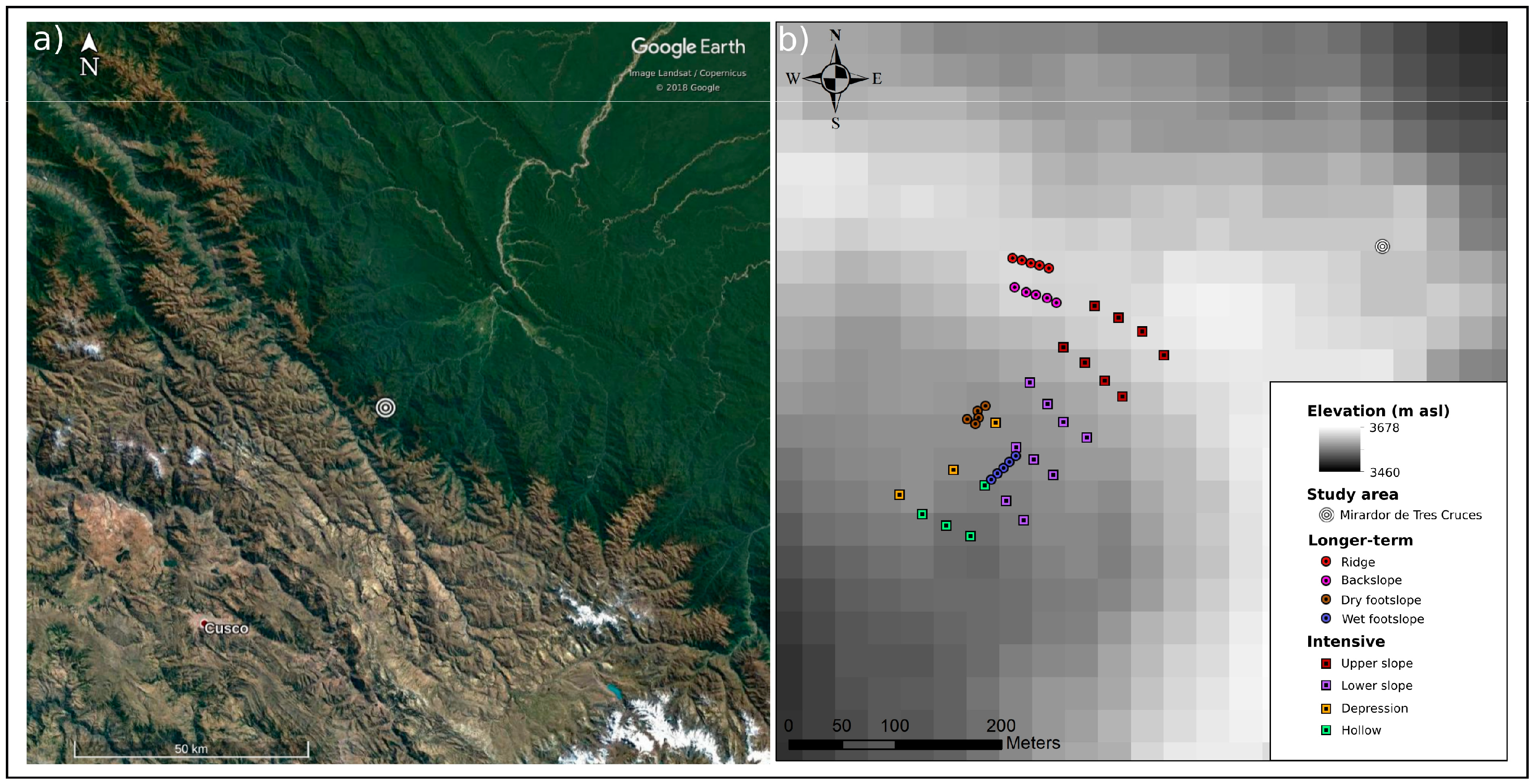
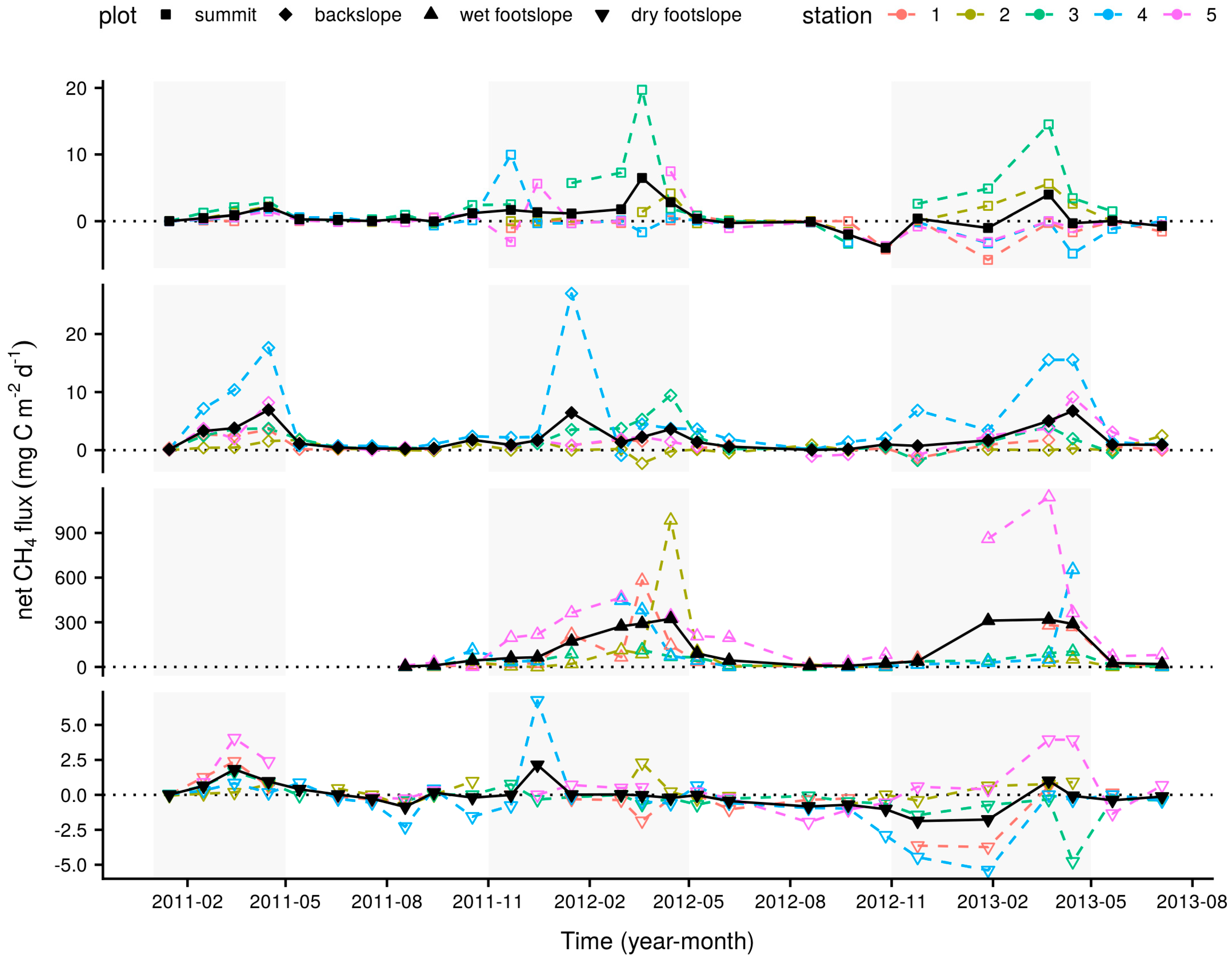
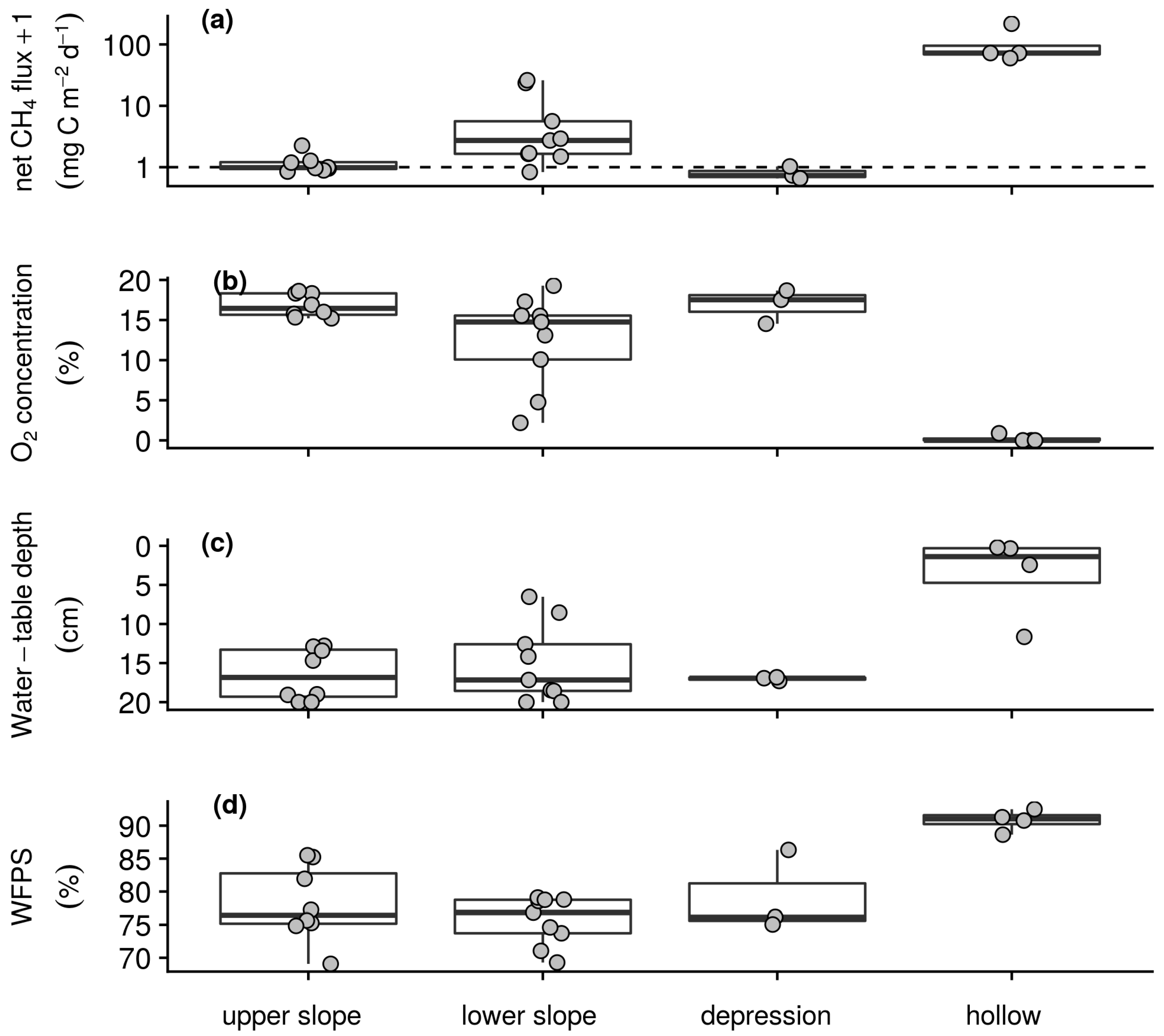
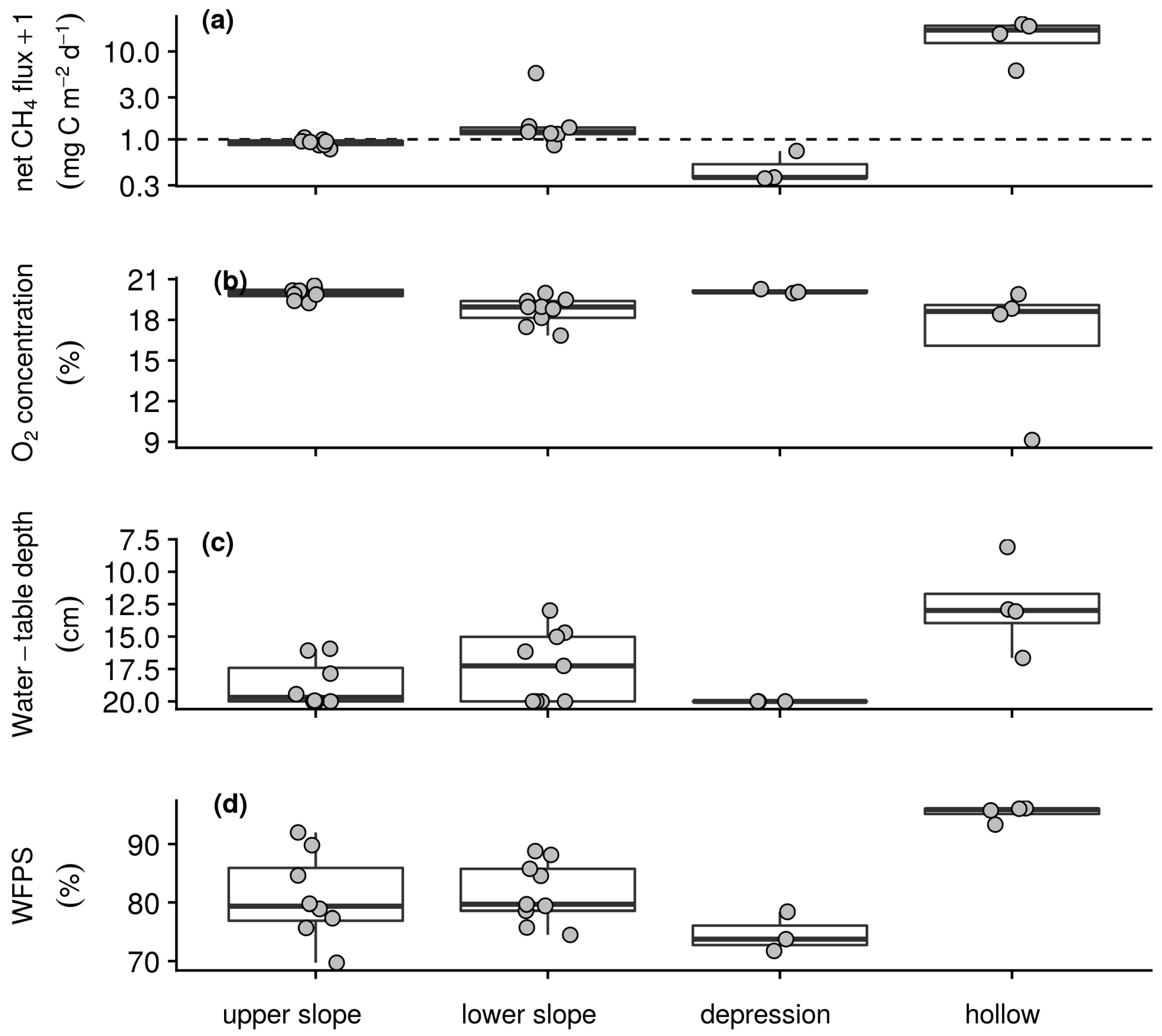
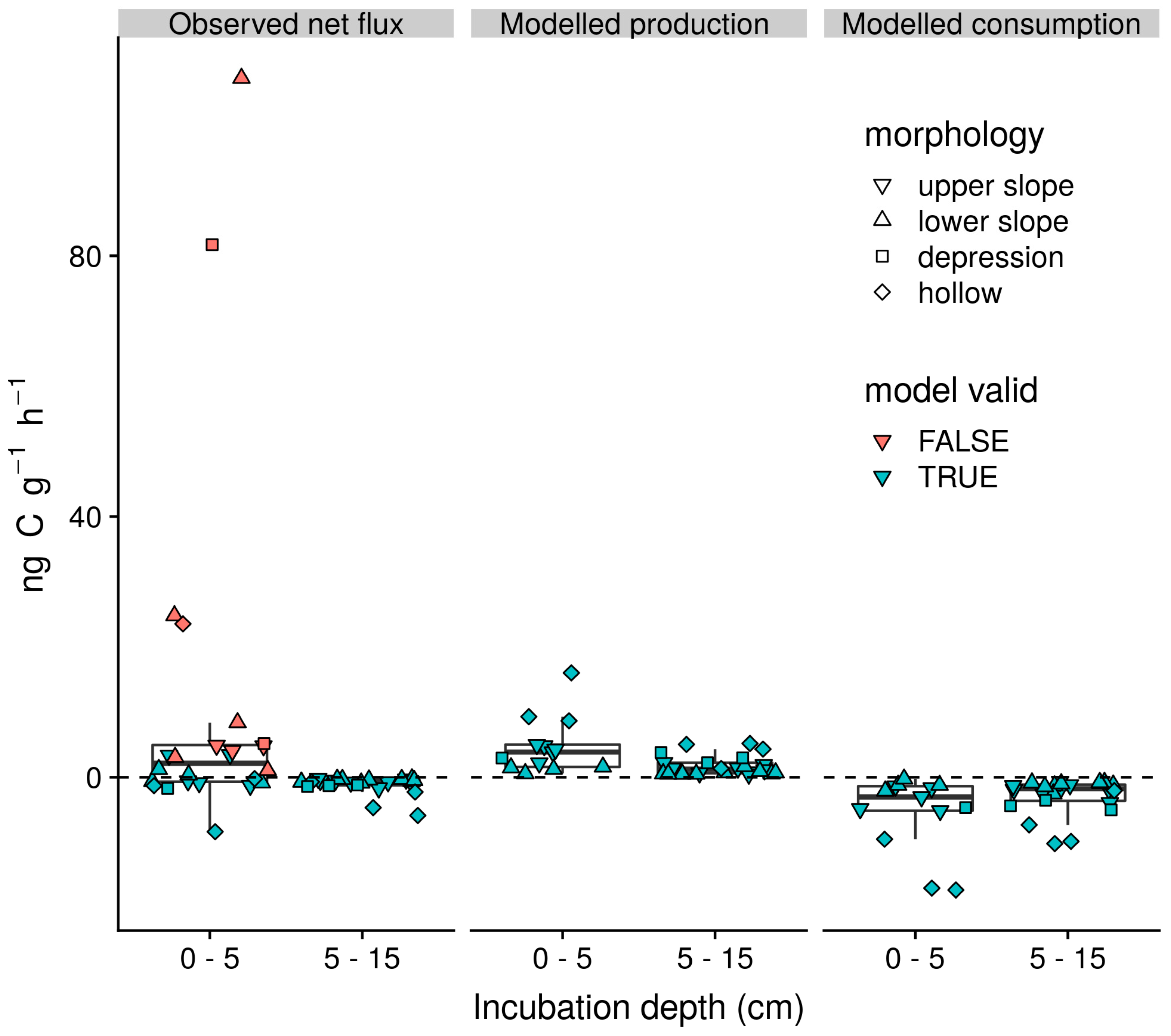
Table 1.
Seasonally aggregated mean monthly net CH4 flux, net CO2 flux, soil O2 concentration, VWC, and soil temperature for each longer-term measurement plot. Following means, values in parentheses indicate the associated standard error and superscript letters indicate within plot significant differences between wet and dry season months (generalised least squares, p < 0.05). The number of observations for each variable can be found in Table S1 of the supplement.
| Plot | Season | Net CH4 Flux (mg C m−2 d−1) | Net CO2 Flux (g C m−2 d−1) | O2 Concentration (%) | VWC (%) | Soil Temperature (°C) |
|---|---|---|---|---|---|---|
| summit | dry | −0.4 (0.36) a | 1.0 (0.15) a | 17.6 (0.81) a | 72.3 (0.74) a | 9.3 (0.33) a |
| summit | wet | 1.6 (0.51) b | 1.2 (0.14) a | 15.5 (0.93) a | 72.7 (0.61) a | 11.6 (0.24) b |
| backslope | dry | 0.7 (0.15) a | 1.3 (0.13) a | 15.3 (1.10) a | 74.0 (0.61) a | 8.9 (0.42) a |
| backslope | wet | 3.2 (0.62) b | 1.7 (0.34) a | 11.7 (2.06) a | 74.0 (0.34) a | 11.7 (0.28) b |
| wet footslope | dry | 27.8 (8.30) a | 2.1 (0.30) a | 9.7 (2.69) a | 76.2 (0.24) a | 9.5 (0.38) a |
| wet footslope | wet | 214.2 (37.46) b | 1.9 (0.21) a | 3.8 (3.82) a | 75.6 (0.31) a | 12.1 (0.36) b |
| dry footslope | dry | −0.3 (0.12) a | 2.3 (0.35) a | 15.7 (1.06) a | 72.6 (0.77) a | 9.6 (0.33) a |
| dry footslope | wet | 0.2 (0.30) a | 1.9 (0.36) a | 9.6 (1.41) b | 74.3 (0.35) a | 11.7 (0.29) b |
The presence of different superscript letters a, b within plots indicates significant differences between wet and dry season for a given variable (generalised least squares, p < 005)
Table 2.
Spearman’s rank correlation coefficients for temporal relationships between mean monthly net CH4 flux and net CO2 flux, soil O2 concentration, VWC, and soil temperature within each longer-term measurement plot. Following the coefficients, values in parentheses indicate the number of observational pairs, * indicates p < 0.05 and ** indicates p < 0.01.
| Plot | Net CO2 Flux | O2 Concentration | VWC | Soil Temperature |
|---|---|---|---|---|
| Summit | 0.56 (27) ** | −0.31 (23) | 0.12 (25) | 0.54 (27) ** |
| Backslope | 0.15 (27) | −0.44 (23) * | 0.31 (26) | 0.53 (27) ** |
| Wet footslope | −0.17 (20) | −0.61 (10) | −0.06 (19) | 0.64 (20) ** |
| Dry footslope | −0.55 (27) ** | −0.23 (23) | 0.31 (26) | 0.56 (26) ** |
Table 3.
Mean topographic, vegetation, and soil characteristics for the intensive seasonal campaign sampling stations by morphological group. Following means, values in parenthesis indicate the associated standard deviation.
Table 3.
Mean topographic, vegetation, and soil characteristics for the intensive seasonal campaign sampling stations by morphological group. Following means, values in parenthesis indicate the associated standard deviation.
| Morphology | Elevation (m asl) | Slope NW–SE (°) | Slope NE–SW (°) | Soil Depth (cm) | Total Grass Biomass (g m−2) | Calama-grostis Biomass (%) | Scirpus Biomass (%) | Juncus Biomass (%) |
|---|---|---|---|---|---|---|---|---|
| upper slope (n = 8) | 3663 (6) | −2 (2.8) | −14 (2.8) | 26 (3.6) | 286.2 (219.62) | 92.8 (5.5) | 5.5 (3.8) | 1.7 (3.6) |
| lower slope (n = 9) | 3641 (5) | −2 (3.6) | −10 (1.5) | 29 (6.4) | 161.4 (91.39) | 57.4 (26.1) | 18.3 (14.0) | 24.3 (32.0) |
| depression (n = 3) | 3634 (5) | 0 (0.6) | −2 (1.5) | 67 (23.5) | 150.4 (86.12) | 59.4 (52.0) | 6.3 (10.8) | 34.4 (56.9) |
| hollow (n = 4) | 3630 (4) | −1 (0.5) | −1 (1.4) | 63 (32.9) | 76.8 (16.25) | 0.0 (0.0) | 16.4 (11.1) | 83.6 (11.1) |
Table 4.
Mean physical and chemical soil properties at 0–5 and 5–15 cm for the intensive seasonal campaign sampling stations by morphological group. Following means, values in parenthesis indicate the associated standard deviation.
Table 4.
Mean physical and chemical soil properties at 0–5 and 5–15 cm for the intensive seasonal campaign sampling stations by morphological group. Following means, values in parenthesis indicate the associated standard deviation.
| Morphology | Depth (cm) | Bulk Density (g cm−3) | Particle Density (g cm−3) | C Content (%) | C:N | pH |
|---|---|---|---|---|---|---|
| upper slope (n = 8) | 0–5 | 0.16 (0.036) | 2.07 (0.101) | 21.3 (3.68) | 14.8 (0.66) | 4.3 (0.29) |
| lower slope (n = 9) | 0–5 | 0.15 (0.062) | 2.03 (0.131) | 20.8 (4.64) | 15.11 (1.36) | 4.1 (0.10) |
| depression (n = 3) | 0–5 | 0.07 (0.013) | 1.62 (0.045) | 38.5 (2.69) | 19.95 (5.80) | 4.7 (0.50) |
| hollow (n = 4) | 0–5 | 0.03 (0.013) | 1.82 (0.099) | 40.8 (1.40) | 27.6 (7.10) | 4.5 (0.70) |
| upper slope (n = 8) | 5–15 | 0.49 (0.108) | 2.30 (0.115) | 12.6 (3.84) | 12.3 (0.22) | 3.9 (0.16) |
| lower slope (n = 9) | 5–15 | 0.47 (0.155) | 2.34 (0.142) | 11.5 (4.07) | 11.6 (0.50) | 4.1 (0.23) |
| depression (n = 3) | 5–15 | 0.16 (0.030) | 1.68 (0.065) | 35.5 (1.38) | 14.1 (1.49) | 4.0 (0.20) |
| hollow (n = 4) | 5–15 | 0.10 (0.088) | 1.75 (0.153) | 37.3 (9.07) | 23.7 (10.80) | 4.0 (0.61) |
Table 5.
Spearman’s rank correlation coefficients for spatial relationships between sampling station mean net CH4 flux and net CO2 flux, soil O2 concentration, water-table depth, and WFPS for the wet (n = 24) and dry (n = 24) season intensive campaigns. Following the coefficients, * indicates p < 0.05 and ** indicates p < 0.01.
| Campaign | Net CO2 Flux | O2 Concentration | Water-Table Depth | WFPS |
|---|---|---|---|---|
| Wet season | 0.00 | −0.88 ** | −0.45 * | 0.50 * |
| Dry season | 0.11 | −0.76 ** | −0.56 ** | 0.62 ** |
© 2018 by the authors. Licensee MDPI, Basel, Switzerland. This article is an open access article distributed under the terms and conditions of the Creative Commons Attribution (CC BY) license (http://creativecommons.org/licenses/by/4.0/).
Share and Cite
MDPI and ACS Style
Jones, S.P.; Diem, T.; Arn Teh, Y.; Salinas, N.; Reay, D.S.; Meir, P. Methane Emissions from a Grassland-Wetland Complex in the Southern Peruvian Andes. Soil Syst. 2019, 3, 2. https://doi.org/10.3390/soilsystems3010002
AMA Style
Jones SP, Diem T, Arn Teh Y, Salinas N, Reay DS, Meir P. Methane Emissions from a Grassland-Wetland Complex in the Southern Peruvian Andes. Soil Systems. 2019; 3(1):2. https://doi.org/10.3390/soilsystems3010002
Chicago/Turabian StyleJones, Sam P., Torsten Diem, Yit Arn Teh, Norma Salinas, Dave S. Reay, and Patrick Meir. 2019. "Methane Emissions from a Grassland-Wetland Complex in the Southern Peruvian Andes" Soil Systems 3, no. 1: 2. https://doi.org/10.3390/soilsystems3010002