A Composite Tool for Forecasting El Niño: The Case of the 2023–2024 Event

Abstract

Remotely sensed data play a crucial role in monitoring the El Niño/La Niña Southern Oscillation (ENSO), which is an oceanic-atmospheric phenomenon occurring quasi-periodically with several impacts worldwide, such as specific biological and global climate responses. Since 1980, Earth has witnessed three strong ENSO events (1982–1983, 1997–1998, 2015–2016). In September 2022, La Niña entered its third year and was unlikely to continue through 2024. Instead, since 2022, forecasts have pointed to a transition from La Niña to a Neutral phase in the summer or late 2023. The onset of El Niño occurred around April 2023, and it is anticipated by sophisticated models to be a strong event through the Northern Hemisphere winter (December 2023–February 2024). The aim of this study is to demonstrate the ability of the combination of two new methods to improve the accuracy of the above claim because El Niño apart from climate anomalies, significantly impacts Earth’s ecosystems and human societies, regulating the spread of diseases by insects (e.g., malaria and dengue fever), and influencing nutrients, phytoplankton biomass, and primary productivity. This is done by exploring first the previous major El Niño events in the period January 1876–July 2023. Our calculations show that the ongoing 2023–2024 El Niño will not be the strongest.

1. Introduction

Walker and Bliss [1] observed that when Tahiti’s air pressure at sea level was stronger than average, Darwin’s was weaker, and vice versa. After several decades, this “Southern Oscillation” (SO) was also linked to a known phenomenon since the 19th century of warmer than average ocean water off the Pacific coast of South America (Peru-Ecuador). This peaks annually around Christmas and is therefore called El Niño (the little boy—the birth of Christ), a name dating to the 1800s. However, this term has been used in more recent years for the enhanced warmings that occur every 3–7 years (measured by the sea surface temperature (SST) along the Peru–Ecuador coast) [2]. The opposite condition is called La Niña [3].

The coupling of these two phenomena provides the pattern of the El Niño Southern Oscillation (ENSO) [4]. Despite its origins in the tropical Pacific Ocean, the climatic effects of ENSO are felt worldwide (e.g., from droughts in Indonesia and Australia to storms and floods in Ecuador and the USA) due to the changes it causes in global atmospheric circulation patterns. For this reason, ENSO is recognized as the primary influencer of natural changes in the Earth’s climate system [5]. Traditionally, a measure of the large-scale variations in atmospheric pressure between the western and eastern tropical Pacific (between Tahiti and Darwin, Australia) is the Southern Oscillation Index (SOI), which indicates the state of the SO, particularly during episodes of El Niño and La Niña [6].

These enhanced interactions between the ocean and atmosphere result in important consequences for people and ecosystems across the globe, with sometimes catastrophic effects on the ecological system [7,8]. These extreme occurrences have the potential to cause secondary impacts on food availability and costs, as well as heatwaves, wildfires, and other intense weather events. These effects can lead to further economic and political ramifications, such as famines and political unrest [9,10]. The biological consequences of an El Niño event also include sudden population growth or decline that can lead to population genetic problems and adaptability to future environmental changes [11]. Also included is the outbreak of epidemics of diseases transmitted by insects, due to the decrease in rainfall and the increase in temperature in various regions of the world (e.g., Colombia), which cause high mosquito breeding rates [12].

While we mostly understand how ENSO works and its effects around the world, we still don’t know how ENSO will change as the planet warms and what its effect on global weather and climate will then be [13]. For example, we know that El Niño is a source of anomalous ocean conditions that lead to specific biological responses that regulate nutrients and phytoplankton biomass, impacting marine life and primary productivity [14]. Effects on higher organisms such as fish, seabirds, and marine mammals are also suggested, but several years of additional observations are required to determine them precisely [15]. In this regard, coral records and other proxies suggest that ENSO has been happening for thousands of years. Studies as well as the most recent Intergovernmental Panel on Climate Change report conclude that there is no agreement among climate models on how ENSO will be affected by climate change [16].

Climate models play a vital role in predicting El Niño events and providing early warnings to mitigate their impact. Scientists use ocean-atmosphere models to simulate El Niño patterns, considering factors like solar activity and volcanic aerosols. Achieving accurate climate forecasts involves understanding current climate conditions, incorporating slow-changing elements of the climate system, and utilizing sophisticated models. Detecting the onset of El Niño requires grasping teleconnections and utilizing various models, including the El Niño–NAE Teleconnection, the Season-Dependent Predictability Barrier for El Niño, and the Multi-Model Prediction System for ENSO. The latter involves a multi-model ensemble of five dynamical coupled models with different complexities, parameterizations, and resolutions to enhance seasonal climate predictions related to El Niño and SO. Despite the challenges, detecting El Niño remains a crucial focus with global implications [11,13,16].

One way to detect the arrival of El Niño is to analyse satellite and ocean measurements of SST. After three consecutive La Niña years, the spring of 2023 saw the return of El Niño, according to data from the Sentinel-6 Michael Freilich and Sentinel-3B satellites (Figure 1). The main purpose of the Sentinel-6 Michael Freilich satellite is to accurately gauge the height of the ocean. On the other hand, the Sentinel-3 satellite is specifically built to measure various aspects such as sea surface topography, sea and land surface temperature, and even colour [17].

Because in its presence, warmer water expands to fill more volume while colder water contracts, ocean warming causes a rise in sea surface height that can be detected by satellite measurements and thus signal the occurrence of El Niño. A commonly used measure of ENSO strength is the mean SST anomaly (or the Oceanic Niño Index-ONI, i.e., the variations of the 3–month running average of the SST) in the Niño–3.4 region of the equatorial Pacific, a box extending from 170° E–120° E and 5° S–5° N (Figure 1 (top)). According to the latest estimates (of 14 December 2023) (Figure 1 (bottom)), El Niño will continue during the Northern Hemisphere winter, while the transition to a neutral ENSO state is favoured in April–June 2024 (with a 60% probability).

The condition for the presence of El Niño is for this anomaly to equal or exceed 0.5 °C, persisting for several months. Glantz and Ramirez [10] suggested that a temperature increase of 0.7 °C serves as a critical threshold signifying the onset of an El Niño event, allowing ample opportunity for policymakers to implement necessary mitigation strategies. When the anomaly exceeds 1.0 °C, it is considered that El Niño is of moderate strength, while 1.5 °C is the threshold for a strong event.

The climate models attempt to predict the features of the upcoming ENSO events to provide in time the necessary reliable information to the population to get safety measures well in advance [18]. However, the predictions provided by the models are sometimes not accurate enough because the ocean-atmosphere system is complex and complicated. For example, on 29 September 2015, the Australian Government Bureau of Meteorology (BOM) reported that “The 2015 El Niño could be the strongest El Niño since 1997–98” and that the 2015–2016 El Niño event “was likely to peak towards the end of 2015” (http://www.bom.gov.au/climate/enso/archive/ensowrap_20150929.pdf, accessed on 10 January 2024). Similar information was also reported on 8 October 2015 by the Climate Prediction Centre, National Centres for Environmental Prediction, NOAA/National Weather Service (http://www.cpc.ncep.noaa.gov/products/analysis_monitoring/enso_disc_oct2015/ensodisc.pdf, accessed on 10 January 2024).

However, Varotsos et al. [19] indicated that the 2015–2016 El Niño was expected to be quite “moderate to strong” and not “one of the strongest on record”, as that of 1997–1998, by applying the new analysis described in detail in [20] on the SOI time series for the period 1876–2015. That analysis employed a non-linear dynamics tool for detecting precursory signals of strong El Niño occurrences. The 2015–2016 El Niño event was “moderate to strong” and not “one of the strongest events on record.”

There are several statistical methods employed to predict El Niño events, such as ENSO Teleconnection Maps, Deep Learning-Based Forecasting, Retrospective El Niño Forecasts, and Benchmarking Prediction Skill, e.g., [9,18].

In this paper, we focus on the already ongoing 2023–2024 El Niño event, which according to model forecasting is expected to be a strong event during the Northern Hemisphere winter (December 2023–February 2024) (e.g., [21]. We attempt to improve the accuracy of predictions made by employing two new algorithms. The first algorithm allows the detection of precursory signals of the ENSO phase through the utilisation of the SOI time series analysis recently developed by Varotsos et al. [20], which has been successfully used to nowcast (i.e., short-range forecasting) the past three strong ENSO events. The second one is a recently developed nowcasting method that is applied to ONI and SOI.

2. Materials and Methods

For our research, we use average monthly SOI values over the period January 1876–July 2023, obtained from the Long Paddock website entitled Monthly SOI Phase 1887–1989 Base (https://data.longpaddock.qld.gov.au/SeasonalClimateOutlook/SouthernOscillationIndex/SOIDataFiles/MonthlySOIPhase1887–1989Base.txt, accessed on 10 January 2024). The SOI dataset, used in this analysis, is calculated using Troup’s formula [13,14], as follows:

SOI = 10 × [PA(Tahiti) − PA(Darwin)]/SDD

(1)

where PA represents the pressure anomaly. As mentioned above, the SOI is calculated by comparing the monthly average air pressure at Tahiti and Darwin, and then subtracting the long-term average of this difference for the specific calendar month (using data from 1887 to 1989 as a basis for normalization purposes) see https://www.longpaddock.qld.gov.au/soi/ (accessed on 10 January 2024) for more details. The Standard Deviation of the Difference (SDD) represents the variability of this difference for the same calendar month during the base period of 1887 to 1989. It’s worth noting that Troup’s monthly SOI from 1876 onwards is derived from the normalized mean sea level pressure difference between Tahiti and Darwin.

In addition, in this study, we use monthly mean values of ONI anomalies from January 1950 to April 2023, obtained from NOAA (https://www.cpc.ncep.noaa.gov/data/indices/oni.ascii.txt, accessed on 10 January 2024).

2.1. Natural Time Analysis of SOI Values

We create a new time series $E_i=({\mathrm{S}\mathrm{O}\mathrm{I}}_i+|{\mathrm{S}\mathrm{O}\mathrm{I}}_{min}\left|\right)\mathrm{w}\mathrm{i}\mathrm{t}\mathrm{h}i=\mathrm{1,2},\dots ,N,$ where ${\mathrm{S}\mathrm{O}\mathrm{I}}_i$(${\mathrm{S}\mathrm{O}\mathrm{I}}_{min}$) is the i-th event (minimum value) of the original SOI dataset and $N$ is the total number of SOI events, over the entire period (January 1876 to July 2023). We then use the technique of “natural time analysis” (NTA), matching each event $E_j$ with the quantity $N_j$ denoting the order of the occurrence $E_j$ against the total number of events within a window of k events, i.e., $N_j$ = j/k, with $j=\mathrm{1,2},\dots ,k$. Thus, we introduce a new sequence of pairs ($N_j$, $E_j$) where $E_j$ > 0, using the order of events as a measure of time instead of the conventional clock time (t) [22,23,24,25].

However, the quantity is as follows:

$$P_j=\frac{E_j}{\sum _{j=1}^k{E}_j},j=\mathrm{1,2},\dots ,k,$$

could be considered as a probability, since $P_j>0$ and $\sum _{j=1}^k{P}_j$ = 1 [22,25], so we try to calculate the entropy of SOI events in the natural time domain as follows:

$$S_k={\sum }_{j=1}^k{P}_j{N}_{j}ln{(N}_j)-\left({\sum }_{j=1}^k{P}_j{N}_j\right)ln\left({\sum }_{i=1}^k{P}_i{N}_i\right)$$

(2)

The entropy $S_k$ is calculated for a sliding window of k-length, each time by 1 month, running the entire SOI time series of the N-events. Then, we again use Equation (2) to calculate the entropy, but this time, considering the time reversal in each window, i.e., ${P’}_j$ = $P_{k-j+1}$, with $j=\mathrm{1,2},\dots ,k$, (see [19,25]). The obtained entropy (${S’}_k$) is different from $S_k$ and the quantity Δ$S_k=S_k-{S’}_k$ indicates the time symmetry breaking; see, e.g., Section 7.1 and Appendix A3 of [25].

Positive values of Δ$S_k$correspond to a decreasing time series in natural time, and when Δ$S_k$ exceeds a certain threshold, extremely small SOI events occur, revealing El Niño (see details in [19,25]).

Furthermore, Varotsos et al. [19,20] suggested that the most useful window size for the above-described analysis is k = 20 events (months). Thus, we herewith calculate Δ$S_{20}$ for the past 20 months, and this window is sliding, each time by 1 month, and run the entire SOI time series of N-events.

We also use the well-known Receiver Operating Characteristics (ROC) method (see [26]) to estimate the most appropriate threshold (for Δ$S_{20}$) that could be used as a forecasting tool for small SOI events. ROC allows [26] the evaluation of predictions in an unbiased manner and is widely applied in many fields, including medicine, see, e.g., [27,28,29]. ROC depicts the “true positive rate” (i.e., the percentage of correctly predicted cases over the total number of (positive) cases to be predicted) as a function of the “false positive rate”, which is the percentage of false alarms over the total number of negative cases. Depending on the number of the available positive and negative cases examined the statistical significance of each point in the ROC plane can be estimated using the method described in [30]. For the case of our study, when Δ$S_{k=20}$ is equal to or exceeds a certain threshold (Δ$S_{thresh}$) during the i-th month of the total period under study, an event low ${\mathrm{S}\mathrm{O}\mathrm{I}}_{i+1}$ (less than or equal to a specific value T) is predicted for the next month. If this is verified, then we have a “true positive prediction”. Conversely, in case Δ$S_{20}$< Δ$S_{thresh}$ and ${\mathrm{S}\mathrm{O}\mathrm{I}}_{i+1}>T$, then we have a “true negative prediction”, while the other two combinations lead to errors (see details in [19]).

2.2. Estimation of the Probability Density Function of Δ$S_{20}$

In order to estimate the probability density function (PDF) of Δ$S_{20}$we employ the kernel density estimator approach, see, e.g., [31]:

$$f_N\left(\Delta S_{20}\right)=\frac{1}{N{B}_N}{\sum }_{i=1}^{N}K\left(\frac{\Delta S_{20}-T_i}{B_N}\right)$$

(3)

In Equation (3), T_i is the observed value of Δ$S_{20}$during the period January 1880-July 2023, and N is the total number of these observations. Following [32], we choose the kernel K(x) = $\left\{\begin{array}{c}\frac{3(1-x^2)}{4},\left|x\right|<1\\ 0,\left|x\right|\ge 1\end{array}\right.$ and B_N = 10.25 $\frac{\sigma }{N^{0.34}}$ with σ the standard deviation of the observed Δ$S_{20}$ values.

2.3. The Modified Natural Time Analysis Method for Nowcasting ONI Anomalies

The Modified Natural Time Analysis (M-NTA) utilized for nowcasting involves the following steps:

Initially, the cumulative number (C_N) of ONI values equal to or exceeding a specific x-value is computed. Subsequently, the logarithm of C_N is plotted against the x magnitude, and regression analysis is conducted on the log(C_N) versus x plot to unveil the distribution of ONI anomalies.

Following this, the NTA is employed to examine exceptional events within the time series of ONI anomalies. By disregarding clock time and focusing on “natural time”, an index is generated representing the order of occurrence of an event divided by the total number of events in the time series [22,23,24,25,33,34]. Consequently, high ONI values (with x ≥ x₂) are identified in the studied time series, and the cumulative numbers C_N1 and C_N2 of ONI values with magnitude x ≥ x₁ and x ≥ x₂, respectively (where x₁ < x₂) occurring after this high ONI value until the end of the time series is calculated.

Ultimately, the M-NTA is utilized to forecast the occurrence rate of future extreme ONI events, based on the estimated mean occurrence rate of the lowest (and most frequent) ONI values.

3. Results and Discussion

3.1. Experience Gained from Forecasting Previous Major El Niño Events as a Guide for Forecasting the 2023–2024 El Niño Using the ‘Natural Time Analysis”

Our first objective is to study the evolution of the current 2023–2024 El Niño based on the conclusions drawn from the forecast analysis proposed by Varotsos et al. [19] regarding the 2015–2016 El Niño. In this context, we apply the method developed in [19,20] to the SOI dataset for the period from January 1876 to July 2023. All SOI values are considered as small, medium, or large SOI events.

Following the classification of the previous El Niño occurrences derived by the BOM (http://www.bom.gov.au/climate/enso/enlist/, accessed on 10 January 2024), we now consider a threshold value $T=-14$(see also Section 2 and Figure 1 of [19]). We herewith present in Figure 2 the true positive rate (i.e., the number of true positive predictions in all cases with ${\mathrm{S}\mathrm{O}\mathrm{I}}_{i+1}$≤ T = −14) versus the false positive rate (i.e., the number of false positive predictions for all cases with ${\mathrm{S}\mathrm{O}\mathrm{I}}_{i+1}$ > −14) for various Δ$S_{thresh}$-values.

It is important to highlight that the optimal prediction method results in a data point located at the upper left corner or coordinate (0, 1), of the ROC space. This point signifies a perfect balance between sensitivity (no false negatives) and specificity (no false positives), achieving 100% accuracy in both aspects. Points located on the diagonal line y = x represent random guesses, with a distribution that hovers around this line for a limited number of trials (refer to [30]). Conversely, points situated above the diagonal signify accurate prediction outcomes (superior to random guessing), whereas points below the diagonal suggest inadequate results (inferior to random guessing).

The obtained ROC curve (for the studied period January 1876 to July 2023) best fits a function of the form ${f\left(x\right)=a}_1$ +$a_2\sqrt{x}+a_3{x}^d$. So, we find that the point$x_0$of the $f$-curve with the maximum distance d(x) from the diagonal line y = x (i.e., d(x) = $\frac{\left|x-(a_1+a_2\sqrt{x}+a_3{x}^d)\right|}{\sqrt{2}}$) is associated with Δ$S_{thresh}$= 0.0035. This value is exactly equal to the Δ$S_{thresh}$-value suggested by Varotsos et al. [19] (for their studied period of January 1878–October 2015). We note that the slope of the tangent line through the point $x_0$of the $f$-curve (i.e., the derivative $f’\left(x_0\right)$) is unity (Figure 2).

Figure 3 illustrates the temporal evolution of monthly SOI events and the entropy change Δ$S_{20}$in natural time under time reversal, from January 2010 to July 2023. To assess if the 2015–2016 El Niño event can be categorized as “very strong” or even more “one of the strongest on record”, we again use the classification of past El Niño events provided by the BOM (http://www.bom.gov.au/climate/history/enso/, accessed on 10 January 2024).

Figure 3 displays the average minimum negative SOI value, depicted by the coloured areas. These areas are accompanied by the 1σ standard deviation bands for two categories: “weak, weak to moderate, moderate, moderate to strong” (green band) and “strong, very strong” (yellow band) El Niño events. We notice in Figure 3 that the monthly SOI events for the period 2015–2016 remain in the green zone and on the yellow border.

Furthermore, looking at Figure 1 in Varotsos et al. [19], it appears that the SOI time series during the period 2015–2017 presents a less pronounced downward trend compared to the corresponding ones during El Niño events of previous periods such as 1982–1983 and 1997–1998 (see Figure 4).

These observations lead to the conclusion that the forecasting analysis suggested by Varotsos et al. [19] has been thoroughly confirmed, and the El Niño event of 2015–2016 was more accurately described as a “moderate to strong” occurrence rather than being labelled as “one of the strongest on record”.

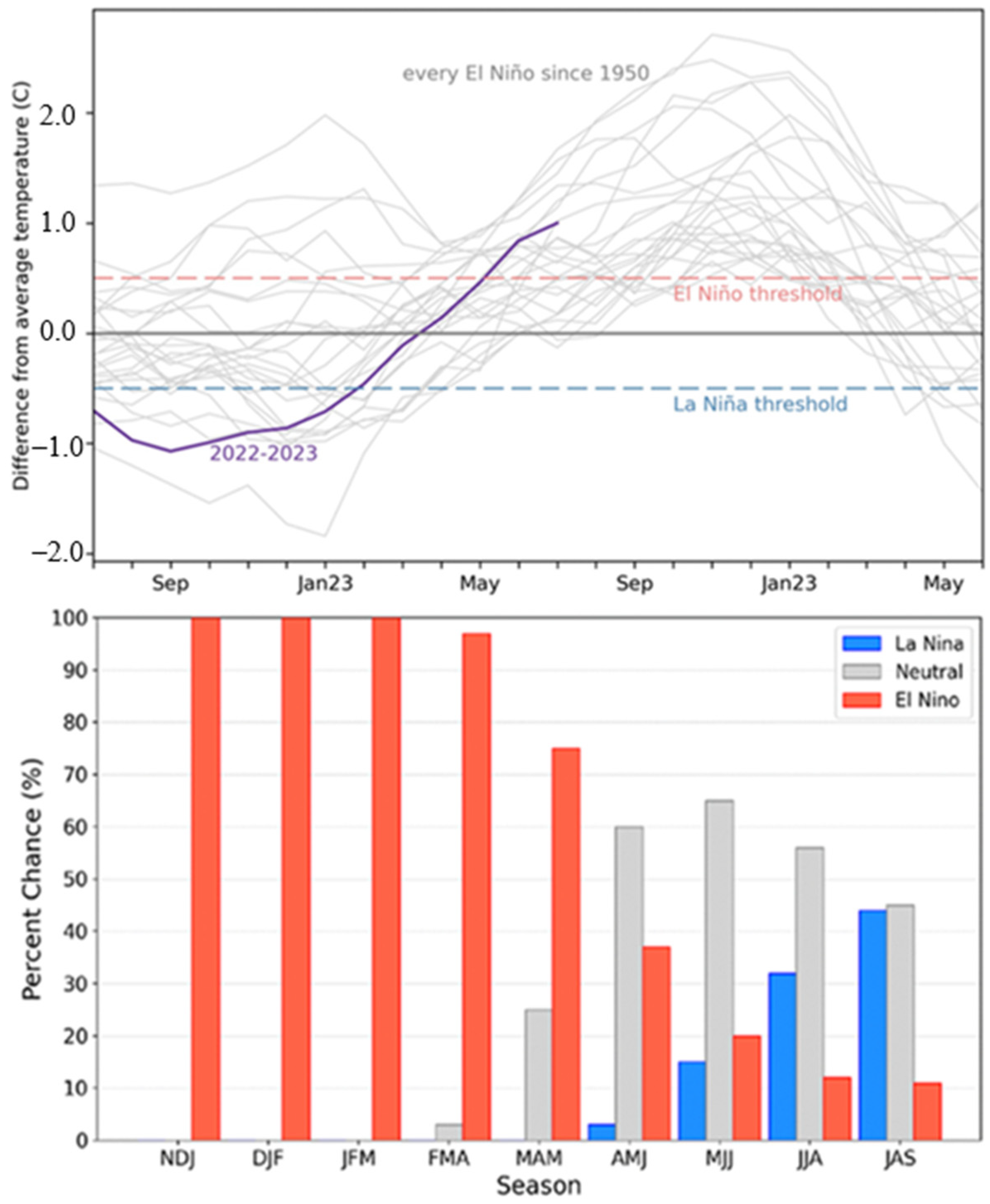
3.2. On the Progress of the 2023–2024 El Niño Event Using the ‘Natural Time Analysis”

Based on our above-described experience from the forecasting of the earlier major El Niño events, we proceed to our second objective to further investigate claims for a very strong 2023–2024 El Niño. However, as clearly shown in Figure 4, the monthly SOI events during January 2021–May 2023 remain above the green zone after an increasing trend, and an abrupt decline occurs in June 2023 without foreshadowing a strong El Niño. Moreover, the variation of Δ$S_{20}$ during the El Niño event of 2023–2024 is not as intense as during the El Niño events of 1982–1983 and 1997–998, and an alarm (i.e., $S_{20}\ge$ Δ$S_{thresh}$) is detected only in May and June 2023.

To estimate the extent of Δ$S_{20}$variation (associated with SOI variation), we plot in Figure 5 the histogram of Δ$S_{20}$and the PDF obtained by the kernel estimation method described in Section 2.2.

3.3. Forecasting El Niño Events Using the “Modified Natural Time Analysis” Applied to ONI

We now investigate the distribution of ONI values, labelled by x, over the period from January 1950 to April 2023, using the Modified Natural Time Analysis (M-NTA) described in Section 2.3. By applying the non-parametric Kolmogorov Smirnov (KS) test, we test the hypothesis Ho: the sample values follow a normal distribution against H₁: the sample values do not follow the normal distribution (Figure 6a). The calculated KS-statistic Dn and the corresponding p-values are 0.043 and 0.076, respectively. From 0.076 > 0.05, we conclude that the dataset fits the normal distribution well at the 95% confidence level.

However, this is inconsistent with the quantile-quantile (Q-Q) plot shown in Figure 6b, which is a graphical method for assessing whether two data sets come from populations with a common distribution. The vertical axis depicts the sample quantiles, while the horizontal axis represents the theoretical quantiles. According to Figure 6b, the ONI values seem to diverge from the normal distribution, and the inconsistency is mainly attributed to the extreme values of the data set. To clarify this point, we apply a newly developed nowcasting method, suggested by Varotsos et al. [30,31,32]. This method is a modified NTA (M-NTA), and its steps are described below:

(1)

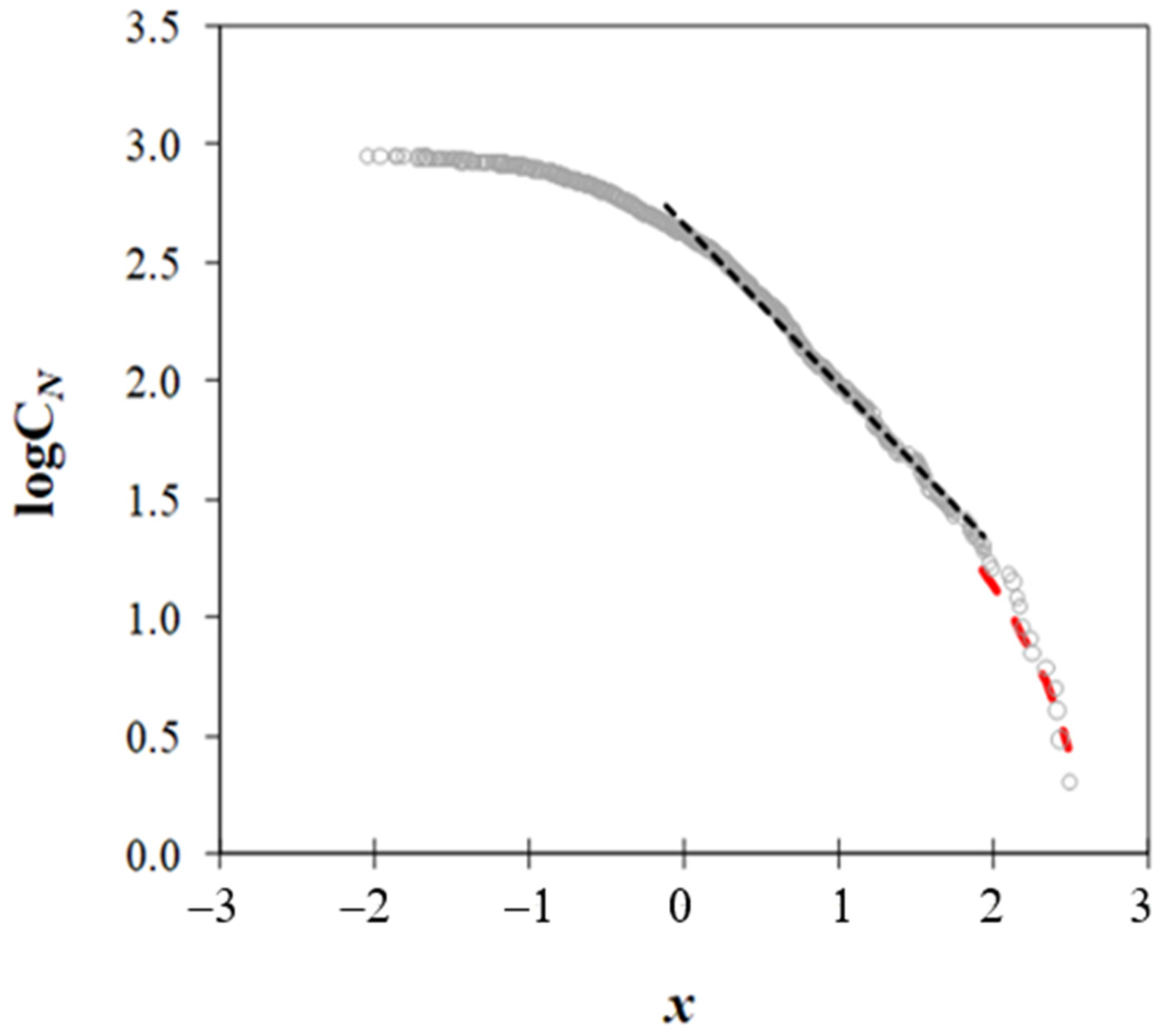
We plot the logarithm of the cumulative number (C_N), see Section 2.3, of the ONI observations, equal to or above a certain x-value versus the x magnitude (Figure 7). For high ONI values, regression analysis reveals a statistically significant linear fit between logC_N and x. The best linear fit is achieved for the range (−0.11, 1.93):

$$\mathrm{l}\mathrm{o}\mathrm{g}{C}_N=a_1+a_0\cdot x$$

(4)

(2)

The F-test (t-test) suggests that the calculated values of R² = 0.99 (a₀ = −0.69 and a₁ = 2.67) are statistically significant (at 95% confidence level), thus giving indications that high ONI values may follow a semi-logarithmic distribution resembling the Gutenberg-Richter (GR) law [34,35,36,37].

(3)

To fit ONI values above rollover (i.e., x ≥ 1.93), we use an upper-truncated GR model developed by [38]

$$C_N’={10}^{a_1}\cdot \left({10}^{a_{0}x}-{10}^{a_0{x}_{\max }}\right)$$

(5)

where the values a₀ and a₁ are derived from Equation (4) and x_max = 2.72 is chosen to obtain the most accurate approximation.

Figure 7. A semi-logarithmic graph illustrating the cumulative number (C_N) of ONI values equal to or exceeding x plotted against x using grey circles The least-squares fit of the GR-scaling is represented by a dashed black line (logC_N = 2.66 − 0.69⋅x with R² = 0.99), whereas the upper-truncated fit obtained from Equation (5) with x_max = 2.72 is depicted by a dashed red line.

Figure 7. A semi-logarithmic graph illustrating the cumulative number (C_N) of ONI values equal to or exceeding x plotted against x using grey circles The least-squares fit of the GR-scaling is represented by a dashed black line (logC_N = 2.66 − 0.69⋅x with R² = 0.99), whereas the upper-truncated fit obtained from Equation (5) with x_max = 2.72 is depicted by a dashed red line.

(4)

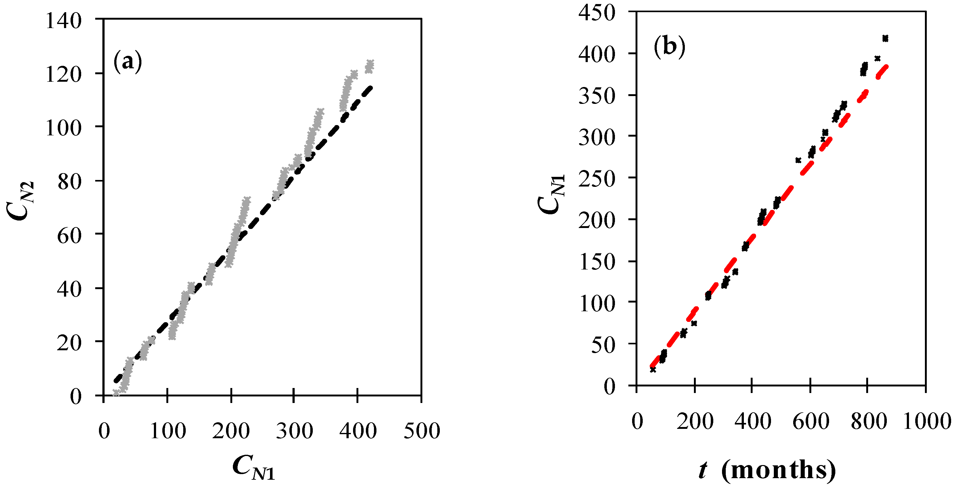
Next, we use the M-NTA (see Section 2.3) to study the exceptional events in the time series of ONI anomalies. The x₁ value is chosen as the average of the ONI dataset (i.e., −0.003), while the value x₂ = 0.826 corresponds to the mean increased by the standard deviation of the dataset.

The above-mentioned technique allows us to precisely test the accuracy of the GR fit by examining whether two values with a constant difference x₂ − x₁ have a constant ratio:

$$\frac{C_{N2}}{C_{N1}}={10}^{a_0\cdot (x_2-x_1)}=\mathrm{constant}$$

(6)

where a₀ is estimated from Equation (4) and C_N1, C_N2 is the cumulative number of ONI values with magnitude x ≥ x₁ and x ≥ x₂, respectively.

(5)

Indeed, we plot the pairs $\left(C_{N1},C_{N2}\right)$ in Figure 8a, and an almost perfect linear fit $f(C_{N1})=A\cdot C_{N1}$ (with A = $0.27$ and R² = 0.97), thus confirming the accuracy of the GR-fit.

(6)

The NTA is also used to forecast the frequency of upcoming extreme ONI events, x₂, by relying on the estimated average occurrence rate of the lowest ONI values, x₁.

To this end, we first plot C_N1 versus the clock time t (during January 1950–April 2023) where a nearly perfect linear fit $h(t)=b\cdot t$ on the pairs $\left(C_{N1},t\right)$ emerges (Figure 8b). The constant $b=0.45\pm 0.04$ is estimated based on the average of the ratio $\frac{C_{N1}}{t}$ and its confidence interval is as follows:

$$\left(b-Z_{a/2}\sqrt{\frac{b(1-b)}{n}},b+Z_{a/2}\sqrt{\frac{b(1-b)}{n}}\right)$$

where n is the count of the pairs $\left(C_{N1},t\right)$ and $Z_{a/2}$ is the critical value of the standard normal distribution at a significance level.

Figure 8. (a) The relationship between the cumulative number C_N2 of high ONI values with magnitude x ≥ x₂ and the cumulative number C_N1 of ONI values with x ≥ x₁ (grey points). A linear fit represented by the dashed black line is shown for the pairs with $f\left(C_{N1}\right)=A{C}_{N1}$, where A = $0.27$ and R² = 0.97. (b) The cumulative number C_N1 of ONI values with x ≥ x₁ is plotted against clock time [in months], over the period January 1950–April 2023 (black dots). The red dashed line is the linear fit for the pairs $\left(C_{N1},t\right)$ with $h\left(t\right)=bt$, where b = $0.45$ and R² = 0.98.

Figure 8. (a) The relationship between the cumulative number C_N2 of high ONI values with magnitude x ≥ x₂ and the cumulative number C_N1 of ONI values with x ≥ x₁ (grey points). A linear fit represented by the dashed black line is shown for the pairs with $f\left(C_{N1}\right)=A{C}_{N1}$, where A = $0.27$ and R² = 0.97. (b) The cumulative number C_N1 of ONI values with x ≥ x₁ is plotted against clock time [in months], over the period January 1950–April 2023 (black dots). The red dashed line is the linear fit for the pairs $\left(C_{N1},t\right)$ with $h\left(t\right)=bt$, where b = $0.45$ and R² = 0.98.

The calculated R² = 0.98 indicates high statistical significance at the 95% confidence level. Subsequently, we aim to forecast the frequency of events $\frac{C_N’}{t}$ and, as a result, the mean time gap between two consecutive occurrences of ONI values with x ≥ x₀ for selected high magnitudes, i.e., $1.74\le x_0\le 2.64$, using the following formula, which is derived from Equation (6), as follows:

$$\frac{C_N’}{t}={10}^{a_0\cdot (x_0-x_1)}\cdot b$$

(7)

where b is seen in Figure 8b (

Table 1. The nowcasted mean inter-event time t [in years] for ONI values with magnitude $1.74\le x_0\le 2.48$ accompanied by the lower and upper limit of the 95%-confidence interval of t. The numbers in black (grey) colour derive from the ONI time series with real (reversed) time evolution.

ONI Value x0	Nowcasted Mean Inter-Event Time t [in Years]	The Lower Limit of the 95% Confidence Interval of t.	The Upper Limit of the 95% Confidence Interval of t.
1.74	3.0 (2.6)	2.5 (2.2)	3.7 (3.2)
1.84	3.5 (3.1)	2.9 (2.6)	4.3 (3.8)
1.94	4.1 (3.6)	3.4 (3.1)	5.1 (4.4)
2.04	4.8 (4.3)	4.0 (3.6)	6.0 (5.2)
2.14	9.2 (8.2)	7.6 (6.9)	11.4 (10.0)
2.24	12.1 (10.8)	10.1 (9.2)	15.1 (13.2)
2.57	51.4 (45.9)	42.8 (38.9)	64.3 (56.0)
2.64	102.1 (91.2)	85.1 (77.3)	127.6 (111.1)

).

It is worth noting that, in the case of extremely high ONI values (with x ≥ 1.93), we use the truncated GR scaling given in Equation (5) (i.e., $\frac{C_N’}{t}=\frac{{10}^{a_0\cdot x_0}-{10}^{a_0\cdot x_{\max }}}{{10}^{a_0\cdot x_1}-{10}^{a_0\cdot x_{\max }}}\cdot b$).

The last step of our survey is to repeat the NTA, this time applied to a new time series, which is generated by the initial ONI time series having reversed its time evolution. The analysis gives similar results (i.e., $f(C_{N1})=0.27C_{N1}$ with R² = 0.99 and b = 0.50 ± 0.04 with R² = 0.995), and the estimated nowcasted mean inter-event time for the selected ONI values is presented in Table 1 (with grey colour).

According to Thompson [13], the phenomenon “El Niño” has arrived, causing major changes to the weather all over the world. It is predicted that either this year or the upcoming year will be the warmest year ever recorded, like what occurred in 2016. Additionally, it is indicated that the strength of the 2016 El Niño event was comparable to the one experienced in 1998 (refer to [16]). The ONI values from October 1997 to January 1998 (i.e., 2.33, 2.4, 2.39, 2.24, respectively), as well as the ONI value from October 2015 to January 2016 (i.e., 2.42, 2.57, 2.64, 2.48, respectively), are seen to be the maxima of the total time series (see Figure 9).

Using the M-NTA, the estimation of the mean inter-event time for the ONI value occurred in November 1997 (i.e., x₀ = 2.4), which is between 17.4 and 26.1 years, a forecast that sufficiently describes the empirical inter-event time from 1997 to 2016 (see Table 1). Furthermore, in December 1982 (i.e., 15 years before December 1997), the ONI value is x₀ = 2.23, which corresponds to the estimated inter-event time (9.8, 14.7) years, revealing a good agreement between the nowcasted and the empirical time. Finally, using Table 1, we can predict that the meantime for the re-appearance of the ONI values observed in November 2015 and December 2015, i.e., 2.57 and 2.64, is expected to be (42.8, 64.3) years and (85.1, 127.6) years, respectively.

Regarding the prediction of the new El Niño event, this is linked to the extreme values of many previous years. For example, in November 1997, we had an extreme ONI-value = 2.40, which, according to the model, is expected to reappear in (17.4, 26.1) years, possibly reaching 2023. On the other hand, from October 2015 to December 2015, extreme ONI values, i.e., 2.42, 2.57, 2.64 arose, which according to the model, may be repeated in [18.9, 28.3] years, (42.8, 64.3) years, and (85.1, 127.6) years, respectively. Therefore, extreme value is difficult to reappear in 2023 (originating from 2015–2016 with an ONI-value ≥ 2.42) but can appear originating from 1997 (with an ONI-value ≈ 2.40).

However, it is very likely that for the winter of 2023–2024, a large ONI-value associated with 2015–2016 will appear since in September 2015 and February 2016, we had a large ONI-value = 2.16 and ONI-value = 2.14, respectively, which according to the model, they will repeat in (8.0, 12.0) years and (7.6, 11.4) years, possibly reaching 2023–2024.

3.4. Forecasting El Niño Events Using the “Modified Natural Time Analysis” Applied to SOI

To confirm the above-mentioned results, we apply the same M-NTA method to the SOI dataset during the period January 1950–April 2023, focusing on the low SOI values that appear to dominate during the three strong ENSO events (1982–1983, 1997–1998, 2015–2016).

Thus, we plot the logarithm of the cumulative number (c_N) of the SOI observations equal to or below a certain x-value against x. For low SOI values, the regression analysis gives a statistically significant linear fit between logc_N and x (i.e., logc_N = a₃ + a₂x) with optimal features in the range of values (−∞, −3.1], where the calculated values of R² = 0.99 (a₂ = 0.07 and a₃ = 2.86) are statistically significant (at 95% confidence level).

Then, we detect the low SOI values (with x ≤ x₂) in the studied time series, and every time a low SOI value occurs, we calculate the cumulative numbers c_N1, c_N2 of the SOI values with magnitude x ≤ x₁, x ≤ x₂, respectively (where x₁ < x₂), that occur after this low SOI value until the end of the time series. The x₁ value is chosen as the threshold of the above-mentioned value range (−∞, −3.1], while the value x₂ = −8.2 is the 20% percentile of the entire dataset.

Plotting the pairs (c_N1, c_N2), a perfect linear fit $f(c_{N1})=A\cdot c_{N1}$ (with A = $0.44$ and R² = 0.99) confirms the accuracy of the GR- fit. We then plot c_N1 against clock time t (during January 1950–April 2023) and a statistically significant (at 95% confidence level) linear fit $h(t)=b\cdot t$ (with b = 0.36 ± 0.04 and R² = 0.98) is revealed.

Finally, using the above results, we forecast the occurrence rate $\frac{C_N’}{t}={10}^{a_0\cdot (x_0-x_1)}\cdot b$ and consequently the average time interval between two successive SOI values with x ≤ x₀. In this regard, we select the low SOI values with −35.7 ≤ x₀ ≤ −19.0, i.e., values like those observed during the three strong ENSO events (

Table 2. The nowcasted mean inter-event time t [in years] for SOI values with a magnitude x₀ from −35.7 to −19.0 accompanied by the lower and upper limit of the 95% confidence interval of t.

SOI Value x0	Nowcasted Mean Inter-Event Time t [in Years]	The Lower Limit of the 95% Confidence Interval of t	The Upper Limit of the 95% Confidence Interval of t
−19.0	3.6	3.0	4.5
−21.3	5.4	4.5	6.8
−21.7	5.8	4.9	7.2
−26.1	12.5	10.4	15.6
−30.0	24.6	20.6	30.6
−31.4	31.4	26.2	39.1
−35.7	66.3	55.4	82.5

).

Using Table 2, we see that the average time for the SOI values observed in October 2015 and January 2016 (i.e., −21.30 and −21.7) to reappear is (4.5, 6.8) years and (4.9, 7.2) years, respectively, while the SOI magnitudes in November 1982 and March 1998 (i.e., −30 and −26.1) correspond to (20.6, 30.6) years and (10.4, 15.6) years, respectively.

However, all these extremely low values seem to not affect the current ENSO event (2023–2024). On the other hand, the January 1983 SOI value (i.e., −31.4) corresponds to (26.2, 39.1) years and could be related to the 2015–2016 ENSO, while the February 1983 SOI value (i.e., −35.7) corresponds to (55.4, 82.5) years and is expected to affect the years after 2038. As for the SOI value of May 2023 (i.e., −15.26), it may be related to the minimum SOI of 2019 (i.e., −14.6).

The aforementioned findings become more crucial considering that the increase in carbon dioxide and other greenhouse gases in the atmosphere has already caused and will continue to cause an increase in the amount of longwave radiation that is trapped in the Earth’s climate system [39]. This has undoubtedly resulted in and will continue to result in an enhancement of the atmospheric greenhouse effect that contributes to global warming [40]. But the warming of the deep ocean waters could hinder the climate recovery expected by current models in some regions, even if we successfully achieve carbon neutrality or net negative emissions [41,42]. Therefore, it is important to scrutinize the findings of this study to promptly mitigate the social and environmental consequences caused by El Niño events by achieving the necessary resilience [43]. This is an immediate priority for the additional reason that the current view is that the frequency and intensity of El Niño events due to climate change will have consequences capable of affecting biodiversity, ecosystem health, local communities, the economy, and the quality of air [44,45,46].

4. Conclusions

Applying NTA and M-NTA to SOI and ONI data, we explored the forecasting ability and accuracy of the three strong ENSO events (1982–1983, 1997–1998, 2015–2016) to derive the characteristics of the ongoing 2023–2024 El Niño event. The main findings that emerged are the following:

(1)

Forecasting analysis performed by both NTA and M-NTA verified that the 2015–2016 El Niño was characterized as a “moderate to strong” event and not “one of the strongest on record”, as various forecasting reports of that period claimed.

(2)

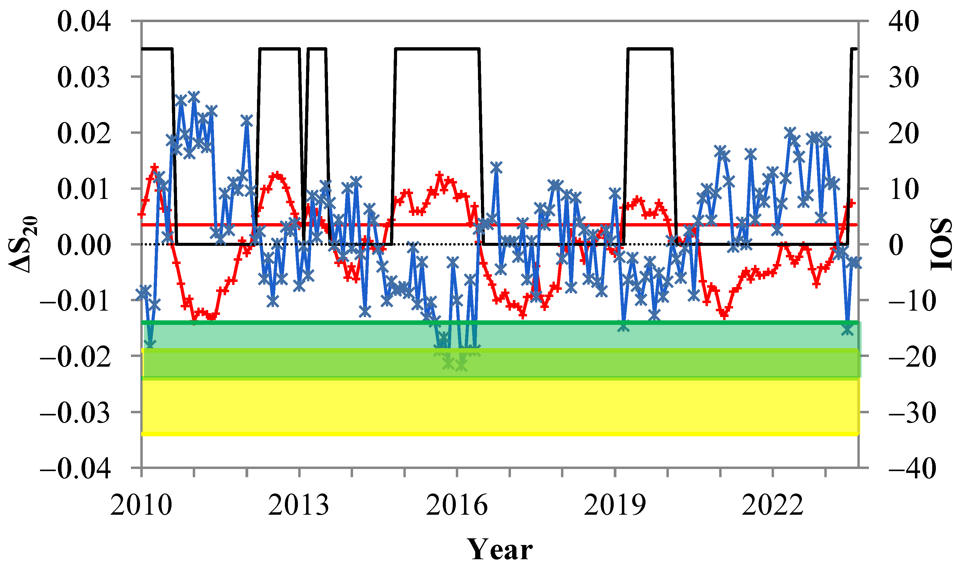
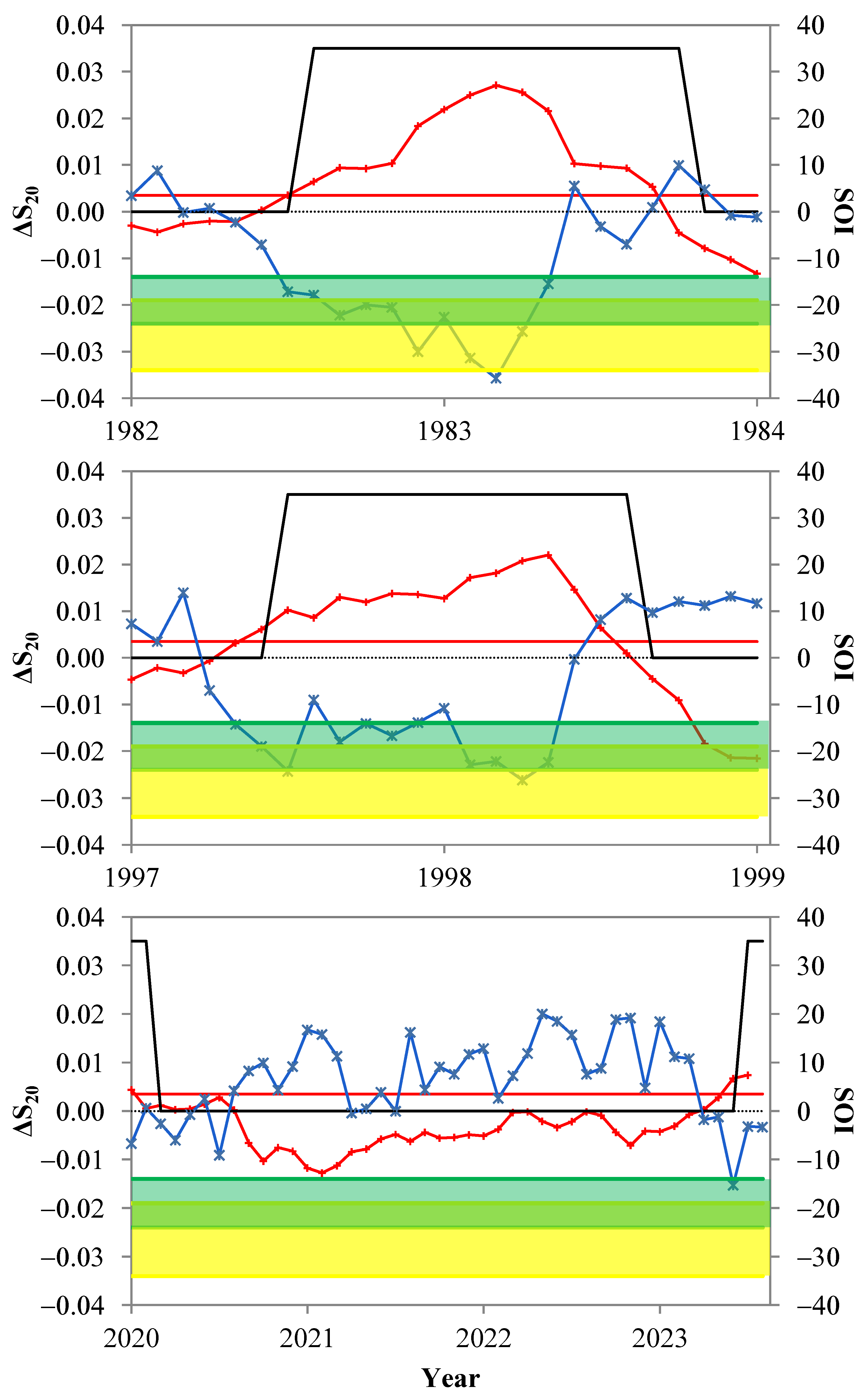
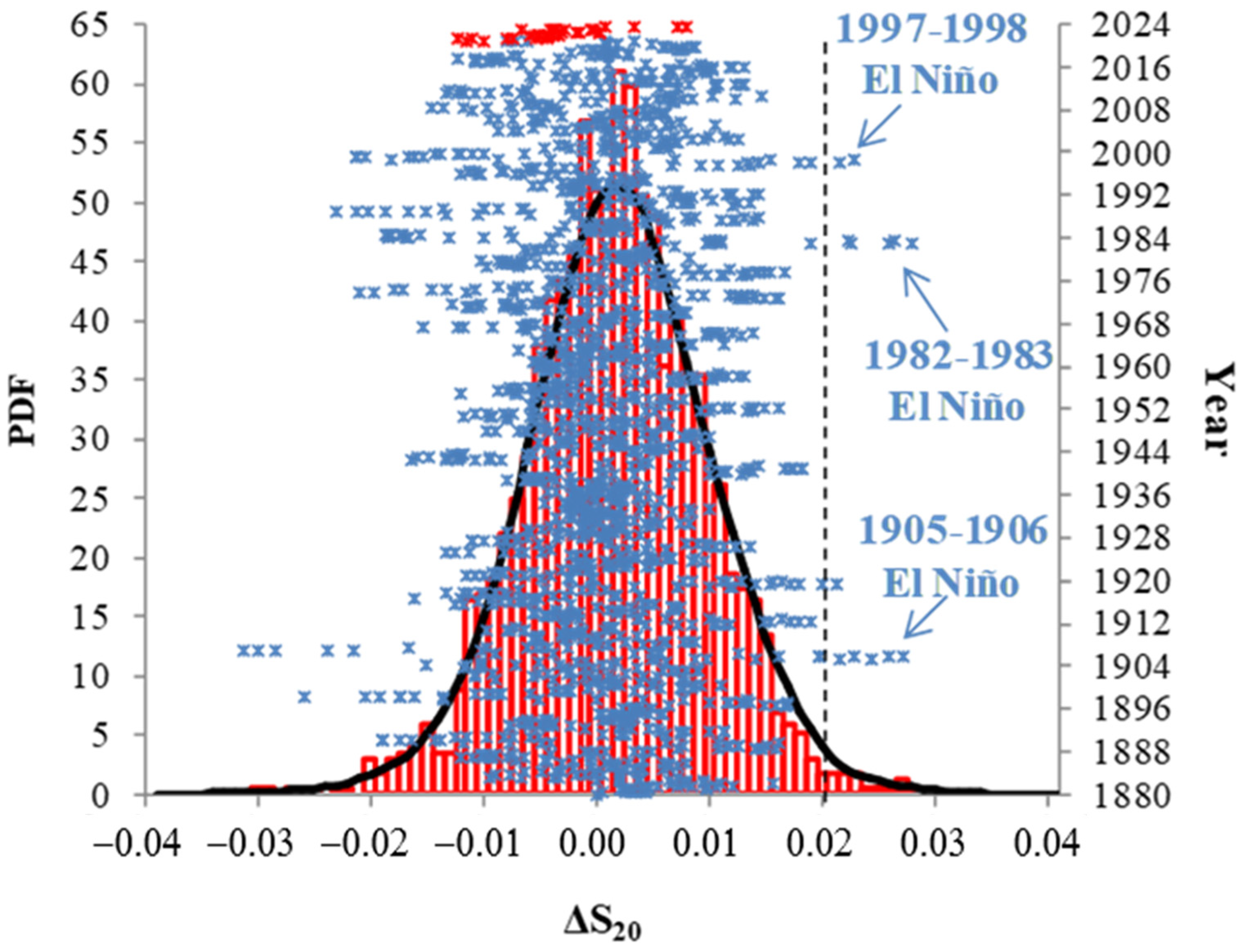
The SOI time series during the period January 2021–July 2023 shows a variance that doesn’t foreshadow a strong 2023–2024 El Niño. Furthermore, the variation of entropy change in natural time during the 2023–2024 El Niño is less pronounced compared to the corresponding ones during past El Niño events. Finally, according to the probability density function of the ΔS_20 dataset, all the values during January 2021–July 2023 remain below the threshold m + s, where m (s) is the mean (standard deviation) of the dataset.

(3)

The M-NTA model appears to adequately estimate the interevent time from 1982 to 1997, two years that correspond to exceptional ONI values of the overall time series. The estimated time of the intermediate event between 1997 and 2016 is estimated to be (17.4, 26.1) years. The average recurrence time of the ONI extremes observed in 2015 was found to be between (18.9, 127.6) years.

(4)

Regarding the intensity of the ongoing 2023–2024 El Niño event, an ONI value of 2.64 occurred only in 2015 (moderate to strong El Niño), and the model predicts a recurrence period of over 85 years. So, it is unlikely to reappear in 2023. Instead, values from 2.14 to 2.40 coming from 1997 or 2016 may appear.

(5)

The extremely low SOI values observed in the last three strong ENSO events do not appear to be related to the ongoing ENSO event (2023–2024). On the other hand, the January 1983 SOI value could be related to the 2015–2016 ENSO, while the February 1983 SOI value is expected to affect years after 2038. The above-mentioned analytical tools may be applied to paleoclimatic data to predict extreme environmental phenomena that may lead to severe ecological impacts [31].

References

1. Walker, G.T.; Bliss, E.W. World Weather V. Mem. R. Meteorol. Soc. 1932, 4, 53–84. [Google Scholar]
2. Power, S.B.; Kociuba, G. The impact of global warming on the Southern Oscillation Index. Clim. Dyn. 2011, 37, 1745–1754. Available online: https://link.springer.com/article/10.1007/s00382-010-0951-7 (accessed on 10 January 2024). [CrossRef]
3. Rasmusson, E.M.; Carpenter, T.H. Variations in tropical sea surface temperature and surface wind fields associated with the Southern Oscillation/El Niño. Mon. Weather Rev. 1982, 110, 354–384. [Google Scholar] [CrossRef]
4. Troup, A.J. The Southern Oscillation. Q. J. R. Meteorol. Soc. 1965, 91, 490–506. Available online: https://rmets.onlinelibrary.wiley.com/doi/abs/10.1002/qj.49709139009 (accessed on 10 January 2024). [CrossRef]
5. Yun, K.S.; Lee, J.Y.; Timmermann, A.; Stein, K.; Stuecker, M.F.; Fyfe, J.C.; Chung, E.S. Increasing ENSO–rainfall variability due to changes in future tropical temperature–rainfall relationship. Commun. Earth Environ. 2021, 2, 43. [Google Scholar] [CrossRef]
6. Neelin, J.D.; Latif, M. El Nino dynamics. Phys. Today 1998, 51, 32. [Google Scholar] [CrossRef]
7. Cai, W.; Ng, B.; Geng, T.; Jia, F.; Wu, L.; Wang, G.; Liu, Y.; Gan, B.; Yang, K.; Santoso, A.; et al. Anthropogenic impacts on twentieth-century ENSO variability changes. Nat. Rev. Earth Environ. 2023, 4, 407–418. [Google Scholar] [CrossRef]
8. Singh, M.; Sah, S.; Singh, R. The 2023-24 El Niño event and its possible global consequences on food security with emphasis on India. Food Sec. 2023, 15, 1431–1436. [Google Scholar] [CrossRef]
9. Ubilava, D.; Abdolrahimi, M. The El Niño Impact on Maize Yields Is Amplified in Lower Income Teleconnected Countries. Environ. Res. Lett. 2019, 14, 054008. Available online: https://iopscience.iop.org/article/10.1088/1748-9326/ab0cd0/meta (accessed on 10 January 2024). [CrossRef]
10. Glantz, M.H.; Ramirez, I.J. Reviewing the Oceanic Niño Index (ONI) to Enhance Societal Readiness for El Niño’s Impacts. Int. J. Disaster Risk. Sci. 2020, 11, 394–403. [Google Scholar] [CrossRef]
11. Gurdek-Bas, R.; Benthuysen, J.A.; Harrison, H.B.; Zenger, K.R.; van Herwerden, L. The El Niño Southern Oscillation drives multidirectional inter-reef larval connectivity in the Great Barrier Reef. Sci. Rep. 2022, 12, 21290. [Google Scholar] [CrossRef]
12. Khanke, H.R.; Azizi, M.; Asadipour, E.; Barati, M. Climate Changes and Vector-borne Diseases with an Emphasis on Parasitic Diseases: A Narrative Review. Health Emerg. Disasters Quart. 2023, 8, 293–300. [Google Scholar]
13. Thompson, A. El Niño May Break a Record and Reshape Weather around the Globe. Scientific American. 21 June 2023. Available online: https://www.scientificamerican.com/article/el-nino-may-break-a-record-and-reshape-weather-around-the-globe/ (accessed on 10 January 2024).
14. Yin, J.; Xu, J.; Xue, Y.; Xu, B.; Zhang, C.; Li, Y.; Ren, Y. Evaluating the impacts of El Niño events on a marine bay ecosystem based on selected ecological network indicators. Sci. Total Environ. 2021, 763, 144205. [Google Scholar] [CrossRef]
15. Barber, R.T.; Chavez, F.P. Biological Consequences of El Nino. Science 1983, 222, 1203–1210. Available online: https://www.science.org/doi/abs/10.1126/science.222.4629.1203 (accessed on 10 January 2024). [CrossRef]
16. WMO. El Niño/La Niña Updates. 2022. Available online: https://public.wmo.int/en/our-mandate/climate/el-ni%C3%B1ola-ni%C3%B1a-update (accessed on 10 January 2024).
17. Hamlington, B.D.; Willis, J.K.; Vinogradova, N. The emerging golden age of satellite altimetry to prepare humanity for rising seas. Earth’s Future 2023, 11, e2023EF003673. [Google Scholar] [CrossRef]
18. Omid, A. Advances and challenges in climate modeling. Clim. Chang. 2022, 170, 18. [Google Scholar] [CrossRef]
19. Varotsos, C.A.; Tzanis, C.G.; Sarlis, N.V. On the progress of the 2015–2016 El Niño event. Atmos. Chem. Phys. 2016, 16, 2007–2011. [Google Scholar] [CrossRef]
20. Varotsos, C.A.; Tzanis, C.; Cracknell, A.P. Precursory Signals of the Major El Niño Southern Oscillation Events. Theor. Appl. Climatol. 2016, 124, 903–912. Available online: https://link.springer.com/article/10.1007/s00704-015-1464-4 (accessed on 10 January 2024). [CrossRef]
21. National Oceanic and Atmospheric Administration (NOAA). El Niño/Southern Oscillation (ENSO) Diagnostic Discussion, Issued by Climate Prediction Center. 2023. Available online: https://www.cpc.ncep.noaa.gov/products/analysis_monitoring/enso_advisory/ensodisc.shtml (accessed on 10 January 2024).
22. Varotsos, P.A. Is time continuous? arXiv 2006, arXiv:cond-mat/0605456. [Google Scholar] [CrossRef]
23. Sarlis, N.V.; Skordas, E.S.; Varotsos, P.A. Similarity of fluctuations in systems exhibiting Self-Organized Criticality. EPL 2011, 96, 28006. [Google Scholar] [CrossRef]
24. Rundle, J.B.; Turcotte, D.L.; Donnellan, A.; Grant Ludwig, L.; Luginbuhl, M.; Gong, G. Nowcasting earthquakes. Earth Space Sci. 2016, 3, 480–486. [Google Scholar] [CrossRef]
25. Varotsos, P.A.; Sarlis, N.V.; Skordas, E.S. Natural Time Analysis: The New View of Time, Part II. Advances in Disaster Prediction Using Complex Systems; Springer Nature Switzerland AG: Cham, Switzerland, 2023. [Google Scholar] [CrossRef]
26. Fawcett, T. An introduction to ROC analysis. Pattern Recogn. Lett. 2006, 27, 861–874. [Google Scholar] [CrossRef]
27. Mandrekar, J.N. Receiver Operating Characteristic Curve in Diagnostic Test Assessment. J. Thorac. Oncol. 2010, 5, 1315–1316. [Google Scholar] [CrossRef]
28. Lalkhen, A.G.; McCluskey, A. Clinical tests: Sensitivity and specificity. CEACCP 2008, 8, 221–223. [Google Scholar] [CrossRef]
29. Hosmer, D.W.; Lemeshow, S. Applied Logistic Regression; John Wiley & Sons, Ltd.: New York, NY, USA, 2000. [Google Scholar] [CrossRef]
30. Sarlis, N.V.; Christopoulos, S.-R.G. Visualization of the significance of Receiver Operating Characteristics based on confidence ellipses. Comput. Phys. Commun. 2014, 185, 1172–1176. [Google Scholar] [CrossRef]
31. Guignard, F.; Mauree, D.; Lovallo, M.; Kanevski, M.; Telesca, L. Fisher–Shannon Complexity Analysis of High-Frequency Urban Wind Speed Time Series. Entropy 2019, 21, 47. [Google Scholar] [CrossRef]
32. Mercik, S.; Weron, K.; Siwy, Z. Statistical analysis of ionic current fluctuations in membrane channels. Phys. Rev. E 1999, 60, 7343–7348. [Google Scholar] [CrossRef]
33. Varotsos, C.A.; Efstathiou, M.N.; Christodoulakis, J. The lesson learned from the unprecedented ozone hole in the Arctic in 2020 A novel nowcasting tool for such extreme event. J. Atmos. Sol.-Terr. Phys. 2020, 207, 105330. [Google Scholar] [CrossRef]
34. Varotsos, C.A.; Mazei, Y.; Novenko, E.; Tsyganov, A.N.; Olchev, A.; Pampura, T.; Mazei, N.; Fatynina, Y.; Saldaev, D.; Efstathiou, M.A. New Climate Nowcasting Tool Based on Paleoclimatic Data. Sustainability 2020, 12, 5546. [Google Scholar] [CrossRef]
35. Zhang, S.; Zhang, Y. The “Natural Time” Method Used for the Potential Assessment for Strong Earthquakes in China Seismic Experimental Site. In Natural Hazards-New Insights; IntechOpen: London, UK, 2023. [Google Scholar] [CrossRef]
36. Gutenberg, B.; Richter, C.F. Frequency of earthquakes in California. Bull. Seismol. Soc. Am. 1944, 34, 185–188. [Google Scholar] [CrossRef]
37. Turcotte, D.L. Fractals and Chaos in Geology and Geophysics; Cambridge University Press: Cambridge, UK, 1992. [Google Scholar] [CrossRef]
38. Burroughs, S.M.; Tebbens, S.F. The Upper-Truncated Power Law Applied to Earthquake Cumulative Frequency-Magnitude Distributions: Evidence for a Time-Independent Scaling Parameter. Bull. Seismol. Soc. Am. 2002, 92, 2983–2993. [Google Scholar] [CrossRef]
39. Begun, R.A.; Lempert, R.J. Climate Reference Periods, Global Warming Levels and Common Climate Dimensions. In Point of Departure and Key Concepts; Climate Change 2022: Impacts, Adaptation and Vulnerability. Contribution of Working Group II to the Sixth Assessment Report of the Intergovernmental Panel on Climate Change; Pörtner, H.-O., Roberts, D.C., Tignor, M., Poloczanska, E.S., Mintenbeck, K., Alegria, A., Craig, M., Langsdorf, S., Loschke, S., Okem, B., Eds.; Cambridge University Press: Cambridge, UK; New York, NY, USA, 2022; pp. 121–196. [Google Scholar] [CrossRef]
40. Pirani, A.; Fuglestvedt, J.S.; Byers, E.; O’Neill, B.; Riahi, K.; Lee, J.Y.; Marotzke, J.; Rose, S.K.; Schaeffer, R.; Tebaldi, C. Scenarios in IPCC assessments: Lessons from AR6 and opportunities for AR7. Npj Clim. Action 2024, 3, 1. [Google Scholar] [CrossRef]
41. Oh, J.H.; Kug, J.S.; An, S.I.; Jin, F.F.; McPhaden, M.J.; Shin, J. Emergent climate change patterns originating from deep ocean warming in climate mitigation scenarios. Nat. Clim. Chang. 2024, 1–7. [Google Scholar] [CrossRef]
42. Cheng, L.; Abraham, J.; Trenberth, K.E.; Boyer, T.; Mann, M.E.; Zhu, J.; Wang, F.; Yu, F.; Locarnini, R.; Fasullo, J.; et al. New Record Ocean Temperatures and Related Climate Indicators in 2023. Adv. Atmos. Sci. 2024, 1–15. [Google Scholar] [CrossRef]
43. Benschop, N.D.; Chironda-Chikanya, G.; Naidoo, S.; Jafta, N.; Ramsay, L.F.; Naidoo, R.N. El Niño, Rainfall and Temperature Patterns Influence Perinatal Mortality in South Africa: Health Services Preparedness and Resilience in a Changing Climate. In Climate Change and Human Health Scenarios: International Case Studies; Springer Nature: Cham, Switzerland, 2024; pp. 333–355. [Google Scholar] [CrossRef]
44. Cordero, R.R.; Feron, S.; Damiani, A.; Carrasco, J.; Karas, C.; Wang, C.; Kramwinkel, C.T.; Beaulieu, A. Extreme fire weather in Chile driven by climate change and El Niño–Southern Oscillation (ENSO). Sci. Rep. 2024, 14, 1974. [Google Scholar] [CrossRef]
45. De Oliveira-Júnior, J.F.; Mendes, D.; Szabo, S.; Singh, S.K.; Jamjareegulgarn, P.; Cardoso, K.R.A.; Bertalan, L.; da Silva, M.V.; da Rosa Ferraz Jardim, A.M.; da Silva, J.L.B.; et al. Impact of the El Niño on Fire Dynamics on the African Continent. Earth Syst. Environ. 2024, 8, 45–61. [Google Scholar] [CrossRef]
46. Rawat, A.; Kumar, D.; Khati, B.S. A review on climate change impacts, models, and its consequences on different sectors: A systematic approach. J. Water Clim. Chang. 2024, 15, 104–126. [Google Scholar] [CrossRef]
Figure 1. (Top): Two–year record of SST in the Niño–3.4 (the temperature anomaly of the surface of the central tropical Pacific Ocean currently defined as the departure from the 1991–2020 average). The grey lines represent all El Niño events since 1950, along with the purple line showing the current event. (Bottom): Official ENSO probabilities for the Niño–3.4 SST index (5° N–5° S, 120° W–170° W), updated 14 December 2023 (Credit: NOAA climate.gov). (https://www.cpc.ncep.noaa.gov/products/analysis_monitoring/enso_advisory/ensodisc.shtml, accessed on 10 January 2024).
Forecasting 06 00011 g001
Figure 2. True positive rate vs. false positive rate (black circles) using Δ S 20 as a predictor for the SOI event of the next month, during the period January 1876 to July 2023. The blue arrow indicates the point of the f -curve (red line) with the maximum distance of the diagonal line y = x. The slope of the tangent line (blue line) through that point of the f -curve is unity.
Forecasting 06 00011 g002
Figure 3. Monthly SOI events (blue line, right scale) as a function of time along with the change of entropy ΔS20 in natural time in a time-reversed pattern (red line, left scale), in the period January 2010–July 2023. The average minimum negative SOI values are illustrated, accompanied by 1σ standard deviation bands denoting “weak, weak to moderate, moderate, moderate to strong” (green band) and “strong, very strong” El Niño events (yellow band), represented by coloured areas. The black line represents the alarm triggered when ΔS20 exceeds the threshold value ΔSthresh = 0.0035 (red straight line). Note: SOI values are shifted by 1 month to facilitate a straightforward comparison.
Forecasting 06 00011 g003
Figure 4. As depicted in Figure 3, exclusively for the El Niño occurrences of 1982–1983, 1997–1998 (the two most intense of the previous century), and the ongoing 2023–2024.
Forecasting 06 00011 g004
Figure 5. The black curve on the left scale represents the PDF of Δ S 20 while the corresponding histogram is shown as red bars on the same scale. These values were obtained from the Δ S 20 time series spanning from January 1880 to July 2023. Additionally, the blue points on the right scale depict the variation of ΔS_20 over time along the vertical axis. Blue arrows indicate the Δ S 20 values that exceed the 99% percentile, p99% = 0.02 of the total dataset (p99% is depicted with the vertical dashed black line). These extremes are characterized by correspondingly strong El Niño events. The red points and label show the Δ S 20 values from January 2021 to July 2023.
Forecasting 06 00011 g005
Figure 6. (a) Histogram for the monthly mean x values of the ONI dataset over the period January 1950–April 2023 obtained from NOAA. (b) Normal Q-Q plot for the studied ONI values.
Forecasting 06 00011 g006
Figure 9. Monthly mean ONI (°C) values over the period January 1950–April 2023 (obtained from NOAA).
Forecasting 06 00011 g009