

Point-Cloud Segmentation for 3D Edge Detection and Vectorization


Laboratory of Photogrammetry, School of Rural-Surveying and Geoinformatics Engineering NTUA, 15772 Athens, Greece
*
Author to whom correspondence should be addressed.
Heritage 2022, 5(4), 4037-4060; https://doi.org/10.3390/heritage5040208
Submission received: 7 October 2022
/
Revised: 17 November 2022
/
Accepted: 5 December 2022
/
Published: 9 December 2022
(This article belongs to the Special Issue 3D Virtual Reconstruction and Visualization of Complex Architectures)
Abstract
:The creation of 2D–3D architectural vector drawings constitutes a manual, labor-intensive process. The scientific community has not provided an automated approach for the production of 2D–3D architectural drawings of cultural-heritage objects yet, regardless of the undoubtable need of many scientific fields. This paper presents an automated method which addresses the problem of detecting 3D edges in point clouds by leveraging a set of RGB images and their 2D edge maps. More concretely, once the 2D edge maps have been produced exploiting manual, semi-automated or automated methods, the RGB images are enriched with an extra channel containing the edge semantic information corresponding to each RGB image. The four-channel images are fed into a Structure from Motion–Multi View Stereo (SfM-MVS) software and a semantically enriched dense point cloud is produced. Then, using the semantically enriched dense point cloud, the points belonging to a 3D edge are isolated from all the others based on their label value. The detected 3D edge points are decomposed into set of points belonging to each edge and fed into the 3D vectorization procedure. Finally, the 3D vectors are saved into a “.dxf” file. The previously described steps constitute the 3DPlan software, which is available on GitHub. The efficiency of the proposed software was evaluated on real-world data of cultural-heritage assets.
1. Introduction
The creation and analysis of 3D data has attracted increasing interest from the scientific community during the last decade. The understanding and analysis of 3D data could provide solutions for perplexing and demanding tasks, e.g., the production of self-driving cars, the automation of the production of 2D–3D architectural drawings and the improvement of the 3D perception of robots. There are several types of 3D data provided to the scientific community for analysis in the form of, e.g., 3D point clouds, textured 3D meshes and voxels. A major challenge in computer vision and photogrammetry is the association of 2D–3D data with a semantic meaning, for instance, the identification and detection of scene objects or the materials of a construction presented in a set of images or in a point cloud, in the same way as human perception. In this regard, several approaches have been developed so far, investigating the semantic segmentation of 2D–3D data. The semantic segmentation of 3D data, such as point clouds and meshes, is still an open issue, especially for complex scenes such as cultural-heritage assets. In general, 2D edges form a low-level semantic information incorporated into several deep-learning architectures to extract image features which may then be used for 2D classification, 2D object detection and 2D semantic-segmentation purposes. A plethora of methods developed so far dealing with 3D point-cloud semantic segmentation exploit various transformations of the cloud such as graphs and voxels or are applied directly on it. Furthermore, deep-learning image semantic-segmentation algorithms are combined with the photogrammetric pipeline to produce semantically rich 3D point clouds [1,2,3]. Additionally, 2D–3D semantic-segmentation techniques are exploited to improve other methods such as 3D reconstruction [4,5].
Architectural drawings such as horizontal floor plans and vertical cross sections constitute a valuable product for a variety of scientific fields such as engineers, archaeologists, and craftsmen. Since ancient times, construction or, indeed, conservation works were based on drawings. The primary role or function of working drawings is to convert design data into construction information and to clearly communicate that information to the building industry, code officials, product manufacturers, suppliers, and fabricators. Keeping track of modifications and/or additions during documentation is a necessary step in obtaining an accurate drawing set for the working system. These drawings are a valuable resource for maintenance and troubleshooting. Up to now, drawings are printed, mainly on paper sturdy enough to be handled outdoors and resistant to natural phenomena. In recent years, however, digital technology has advanced remarkably and, consequently, all drawings, 2D or even 3D, are produced and disseminated in digital form. Either in vector or raster format, 2D drawings can, nowadays, be displayed on flat screens of laptops, tablets or even smartphones. However, this display does not fully appeal to field experts as expected. Hence, 2D drawings are still necessary and required, as by creating a drawing more than simply presenting a captured 3D data set, an interpretation of the subject can be provided [6].
- Accessible, platform-independent information. There are many cases when site-work steps beyond the workstation or laptop; this may be due to cost, format compatibility or simple practicality.
- Clarification of complex 3D spaces by use of plan, section or perspective views.
- Simplicity by showing selected information pertinent to a given project.
- Reliable perception of scale, a printed plot, either dimensioned or with a scale, allows consistent shared experience of information, etc.
Nowadays, the creation of 2D–3D architectural drawings is a manual and time-consuming process. Moreover, the completeness in a drawing requires careful examination of the structure not covered by surface recording methods such as photogrammetry or laser scanning. Additionally, the scientific community has not proposed a fully automatic method for the construction of such drawings so far, regardless of the indispensable need in many scientific fields. In this study, a 3D edge-detection approach which leverages 2D edge semantic information is presented. The proposed 3DPlan algorithm which is available
on GitHub (https://github.com/thobet/3DPlan (accessed on 15 September 2022)) can also be exploited using high-level semantic information such as image semantic segmentation, instance segmentation and panoptic segmentation, instead of edge maps, and, thus, may be used in various applications.
Thus far, semantic-segmentation algorithms in 2D space have been investigated more than those in 3D space. Therefore, several approaches exploit such methods to firstly detect and then project the 2D semantic information into 3D space [7,8,9]. For example, if the images are available, image semantic-segmentation algorithms are applied and then the 2D semantic information is projected into 3D space. If the images are not available, firstly, the 3D model is artificially “photographed” from various positions, i.e., 3D–2D projection; then, 2D semantic-segmentation algorithms are applied to the images and, finally, the 2D semantic information is projected back into 3D space. Several applications in drawing creation could exploit 3D–2D line detectors such as the creation of drawings of building facades or the creation of drawings using aerial images instead of terrestrial.
The scope of this effort is to propose a 3D edge-detection algorithm and to investigate the exploitation of those 3D edge points to produce 3D vectors, a major step towards the automation of the production of 2D–3D architectural vector drawings, which will still be required by conservation experts for years to come. To be more specific, the 3DPlan algorithm detects the 2D edges on each RGB image of a given dataset. Then, it enriches the given RGB images with an extra channel which contains the 2D edge semantic information produced in the previous step. The four channel images are passed into the Agisoft-Metashape [10] or the Mapillary-OpenSfM [11] software and a semantically enriched dense point cloud is produced. Finally, the edge points of each edge are grouped and isolated using their labels carried by the semantically enriched point cloud. Finally, the 3D vectors are created using the detected groups of edge points and saved into a “.dxf” file. The steps described are executed automatically using the 3DPlan software. An illustration of the general idea of the 3DPlan software is presented in Figure 1.
The rest of the paper is organized as follows: Section 2 presents the related work, including the traditional and deep-learning 3D edge-detection approaches presented in the literature. The materials and methods are outlined in Section 3. In Section 4, the results using the 3DPlan algorithm are presented, exploiting various datasets as well as testing different parameter combinations. Section 5 presents a discussion of the results, the contributions of the proposed algorithm as well as the parts requiring further investigation. Finally, in Section 6, some conclusions for the proposed algorithm are drawn.
2. Related Work
The general idea of this research is the 3D edge detection for automated 2D –3D vector drawing construction. Several methods developed so far investigate the 3D edge-detection task, a crucial step before the 3D edge-vectorization procedure. These methods can be summarized into two categories, the direct and indirect. On the one hand, the direct methods initially clean the point cloud of the unnecessary parts and the random noise present. Then, the remaining points are grouped into clusters which are exploited to extract the desired 3D edges. On the other hand, indirect methods transform the given point cloud into images on which the 2D edges are detected and then projected back to 3D space, resulting in the coveted 3D edges. Model-fitting techniques are usually involved with 3D edge-detection methods. Bienert [12] introduced an edge-vectorization and dimension approach exploiting smoothed point-cloud profiles. The profile is determined by cutting the given point cloud with a plane parallel to an “origin plane” defined by XY, XZ, YZ or an arbitrary plane and with specific thickness, and is smoothed using a line fitting approach.
A plethora of 3D edge-detection methods presented in the literature exploit plane-intersection techniques. Nguatem, Drauschke and Mayer [13] presented an approach which detects window and door boundaries in 3D space using plane intersection and approximate templates of the desired shapes. Lin et al. [14] introduced the line-segment-half-planes method which uses plane intersection to detect 3D line segments. The given point cloud was projected into several groups of images while the group that fully describes the object of interest was selected. Then, the 2D line segments were detected, applying the LSD [15] algorithm. The extracted lines were filtered to remove the erroneous ones and the remaining lines were projected back into 3D space in a “V” shape. The two non-parallel planes of each projected “V” shape were extracted while their intersection is the desired 3D edge. Mitropoulou and Georgopoulos, Ref. [16], presented an approach which detects 3D edges using plane intersection and the PCL library [17]. The planes are detected by calculating the fitted plane to each of the point triplets in the given point cloud. The planes with the most inliers are selected, and the 3D edges are produced via plane intersection.
Apart from plane intersection, planes could be used to detect 3D edges applying different techniques. Bazazian, Casas and Ruiz-Hidalgo [18] proposed an approach which extracts sharp edges in point clouds exploiting a statistical method in combination with plane fitting. More precisely, the given point cloud was segmented into regions using the kNN algorithm and then a plane was fitted to each segment using the least squares. Afterwards, the covariance matrix of each region as well as its eigenvalues and eigenvectors were calculated. The 3D edges were detected determining if a point lies on an edge or on a plane, using the surface variation formula.
The statistical quantities and matrices, e.g., normal vector and covariance matrix, derived from a set of points, constitute worthwhile information useful to segment those points into groups describing each of the object’s planes. Lu, Liu and Li [19] presented a fast method for 3D line extraction exploiting statistical quantities and matrices. Initially, the given point cloud was decomposed into smaller groups. To achieve that, a region-growing and a region-merging technique were implemented iteratively aiming to accurately detect each of the object’s planes. Those steps were applied calculating the covariance matrix for each region and exploiting its eigenvalues and eigenvectors. Finally, the points of each plane were projected on an image, an edge-detection algorithm was applied, and the detected edges were projected back into 3D space. Dolapsaki and Georgopoulos [20] presented a method in which the desired 3D edges are extracted using oriented high-resolution digital images, the relationships of the analytical geometry and the properties of planes in 3D space. The final 3D edges, in their true position in 3D space, are detected in the available point cloud by applying some constraints. The provided method is semiautomated while the 3D edges are detected with under 1 pix accuracy, using a calibrated camera.
Point clouds can be collected using either image-based or laser-scanning techniques. Both approaches have advantages and disadvantages while, depending on the application, one or both can be implemented. Alshawabkeh [21] proposed a 3D edge-detection method using data from both image-based and laser-scanner techniques. Firstly, the point cloud produced by the laser scanner was converted into a set of depth images. The specifications of the depth images are considered with respect to the captured RGB images. The main goal of this approach was to identify the cracks presented on the facade of the Treasury monument of Petra in Jordan. Thus, the Canny edge detector [22] was implemented on the RGB images to extract the presented cracks. Finally, the found cracks were projected into the 3D space using the depth information provided by the produced depth maps. Apart from the RGB images, the Canny edge detector can be applied directly to range images, generated from point clouds collected by laser scanners, and then reprojected into 3D space [23].
In some applications, 3D edges are used as an abstract representation of shapes. During 3D reconstruction procedures, such methods are commonly used as an alternative to the time-consuming MVS procedure, aiming to generate a group of 3D edges which fully describes the object of interest. An approach was presented by Hofer et al. [24] in which a line-matching method is implemented exploiting the principals of epipolar geometry. Each 3D line is determined using a depth estimation procerdure while the line direction is calculated using the singular value decomposition technique. Finally, a bundle-adjustment technique is provided optionally aiming to produce a more accurate 3D line model. Bazazian and Parés, [25] presented a capsule network, named EDC-Net, which predicts if a point lies on an edge or not, in 3D space. EDC-Net was initially trained using a fully supervised learning approach in combination with the ABC [26] dataset. The generated model was considered as a pretrained model and, thus, was fine-tuned using a weakly supervised transfer learning approach and the ShapeNet [27] dataset. Qi et al. [28,29] proposed an innovative deep-learning architecture, named PointNet, which was applied on the 3D object-detection, 3D part-segmentation and 3D semantic-segmentation applications with remarkable results. The PointNet architecture was the first applied directly to 3D point clouds, introducing a new era in 3D point-cloud analysis. Liu et al. [30] introduced an end-to-end trainable deep network architecture which automatically generates a 3D graph representation of a given 3D point cloud of man-made polyhedral objects such as furniture, mechanical parts, or building interiors, etc.
Building information models (BIMs) are used in point-cloud vectorization methods. Chuang and Sung [31] proposed a learning approach for point-cloud vectorization, which includes a “Feature Extraction” and a “Vectorization” procedure. The approach leverages BIM models during the training process to associate each point with attributes. To be more specific, the approach produces 3D dense point clouds from BIMs which include not only the geometric information but also a semantic meaning, e.g., walls, columns etc., exploiting the information incorporated into the BIM. The test of the proposed approach was conducted using simple 3D dense point clouds, i.e., without semantic meaning, and a plethora of metrics, e.g., recall, precision etc, as well. Additionally, Bassier et al. [32] labeled 3D vector models using an automated approach. The proposed method contains various steps. Firstly, the user defines a set of parameters regarding the data under consideration. Then, the data are cleaned from the noise present and the planar surfaces are segmented. Afterwards the “initial labelling” step is performed using some rules. The horizontal planes are classified into five sub categories, e.g., floors, furniture, etc., and the vertical planes into two subcategories, i.e., wall and unidentified. Fourthly, the labels produced are enhanced for better results. Then, an automated approach gives the opportunity to detect windows and doors. Finally, the labeled data are exported according to their label. The authors state that the disadvantage of the proposed approach is that it cannot be implemented using complex surfaces characterized by a plethora of details and small parts. The described approaches assume that a BIM model is already available. Several approaches developed so far investigate the Scan-to-BIM problem proposing semi-automatic [33] and automatic approaches [34]. Macher et al. [33] proposed a semi-automatic reconstruction approach of indoor point clouds acquired by laser scanner. The authors stated that point-cloud quality plays a significant role during the process and presented a recommendation list of steps to achieve high-quality point clouds using laser scanners. The proposed approach can be divided into two main categories, point-cloud segmentation and 3D reconstruction of walls and slabs. When the reconstruction is performed, a file in the IFC format is exported in which the walls and slabs are included. Finally, an evaluation procedure was conducted using datasets which were not included in the development part. Ochmann et al. [34] proposed an automatic 3D reconstruction approach, in which the main goal is to assign a label to each cell either as “room” or as “outside area”. The proposed method firstly detects planes using the RANSAC algorithm. The parameters used by RANSAC are defined according to the quality of the used indoor point cloud. Then, a point-cloud cleaning method is applied to eliminate the outdoor points collected by the scanner due to building openings such as windows and doors. Afterwards, an automatic binary-classification approach is implemented to classify each point as a “room” point or “outside area” point. Thereafter, two sets of candidates for wall and slab surfaces are extracted. Next, pairs of contrary surfaces are detected, which are characterized as walls by approximately matching parallel surfaces with contrary normal vectors. The wall candidates are used to create a 3D cell complex. Finally, the result is improved using several probabilistic and optimization steps and then it is exported. Each cell in the exported file is assigned to one room or the outside area. The described reconstruction process was evaluated using synthetic and real-world datasets of the construction domain. It is worth noting that the creation of simple BIM models is not a time-consuming process in the construction domain if the building is not characterized by details and heterogeneity. Thus, the BIMs are usually exported into the construction domain in which the buildings are characterized by simpler geometric shapes than the detailed cultural-heritage assets, e.g., monuments. Additionally, the 3D reconstruction of buildings in construction is conducted for entities such as walls, floors and slabs, which are usually characterized by continuous and smooth surfaces. Finally, the construction becomes even more difficult when information such as the materials and thickness of the structures should be included to BIMs.
Obrock and Gülch, [35] presented a method for producing semantically enriched point clouds of interiors, combining deep-learning techniques with photogrammetry. More precisely, a classifier was trained to segment images of interiors into several objects such as floor, doors, windows, etc. Then, the blue channel of each image was replaced by a new channel containing the corresponding ID number for each pixel. One additional variation in this step was mentioned, in which a new channel carrying the semantic information could be added to the existing images as a fourth channel, but, as they mentioned, this was not applied due to technical issues. A vital disadvantage of the proposed method was the production of false color point clouds due to the missing blue channel. Thus, Gülch and Obrock [3] proposed an improved method either in the deep-learning or the photogrammetric part. Firstly, a new deep-learning network was trained using manually produced ground-truth data as well as the DeepLabv3+ [36] architecture instead of FCN-8s [37], producing more accurate semantic-segmentation results than the previous approach. Additionally, the photogrammetric procedure was improved by proposing a two-step approach which generates both a true-color and a semantically enriched point cloud. To be more specific, the SfM algorithm was executed using the original RGB images calculating the relative translation and rotation of each image to the referenced one. The calculated parameters, i.e., the exterior orientation of the images, were exploited to reproject the semantic images generating the semantically enriched point cloud. Finally, the obvious lines, i.e., the intersection of the wall with the floor, were extracted using a heat map and applying the Hough–Transform algorithm. Obviously, the proposed approach requires the generation of a dense point cloud, which is a time-consuming process, twice to produce the true colors and the semantically enriched point clouds. Pellis et al. [2] proposed a new workflow for 3D point-cloud semantic segmentation for cultural-heritage buildings, using photogrammetric and dense image-matching principles. The proposed workflow contains two major steps: firstly, the images are semantically segmented using DeepLabv3+ and secondly, the semantic information is projected into 3D spaces exploiting image masks. Finally, a 3D semantically enriched dense point cloud is produced, for each semantic category.
Edge detection is a fundamental computer vision problem. Xie and Tu [38] proposed a deep-learning method for 3D edge detection called Holistically-nested Edge Detection (HED), which leverages convolutional neural networks (CNN). According to the authors, the HED algorithm outputs better results than the Canny edge detector. Poma, Riba and Sappa, [39] presented an interesting deep-learning-based 2D edge detector, named DexiNed, which produces thin edge maps and can be applied to any image without a previous training procedure. A comparison between the detected 2D edges using state-of-the-art models [38,40,41,42] and DexiNed is presented by the authors, providing useful information for the performance of such methods. Segmentation techniques on point clouds are divided into four categories (i) edge-based, (ii) region-growing, (iii) model-fitting and (iv) clustering [8]. Edge-based methods transfer edge-detection information from images to 3D point clouds aiming to describe the shape of the presented objects. Thus, the 3D point cloud is segmented into smaller parts describing the objects. Bhanu et al. [43] detect 3D edge points using several methods such as gradient computing and line fitting, while they state that the 3D edge points constitute valuable information for 3D shape-recognition purposes.
However, the scientific community has not proposed a fully automatic approach to produce architectural vector drawings yet, in comparison with the unquestionable need from a diversity of scientific fields. In this effort, an edge-based 3D point-cloud segmentation approach exploiting SfM-MVS algorithms is presented to detect 3D edge points and to investigate the automation of the construction of 2D and 3D architectural drawings.
3. Materials and Methods
The motivation of the 3DPlan algorithm is its contribution to the unsolved problem of the automation of the construction of 2D–3D architectural vector drawings. The proposed methodology presents an efficient pipeline for the extraction of 3D edges from point clouds using 2D edge semantic information from digital images. The major steps of the proposed methodology are
- The enrichment of the RGB images with their edge maps constructing four-channel images;
- The usage of the four-channel images into image-based 3D point-cloud production workflows;
- The separation of the 3D points into edge and non-edge points;
- The 3D vectorization of 3D edge points.
3.1. Edge Maps and the Creation of Four-Channel Images
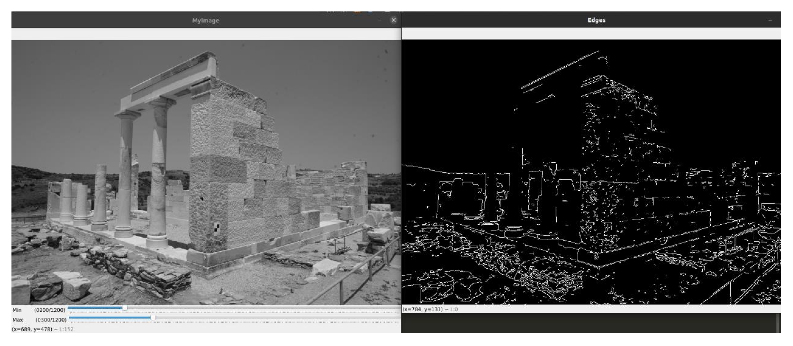
The quality of the detection of the 3D edges is strongly dependent on the quality of the 2D edge maps. However, this effort is focused on the construction of a general software which will be used as the base towards the automation of the production of 2D–3D architectural drawings, and not to investigate the best 2D edge-detection technique, neither the traditional nor the more sophisticated, e.g., DexiNed [39], etc. The 3DPlan software receives the edge semantic information in two ways (i) using a live-Canny implementation which is a user-guided implementation of the Canny algorithm or (ii) using predefined edge maps (an external semantic source). More concretely, using the live-Canny implementation, two windows are opened automatically and the user defines the Canny hysteresis thresholding parameters with the provided bars. The edge map is updated live in the first window while the second one displays the image under process. When the user is satisfied about the depicted edge map, terminates the process. The two windows of the live-Canny are depicted in Figure 2. On the other hand, the external semantic source enables the combination of the given images with predefined edge maps and, thus, the user is not restricted to using Canny algorithm by the providing semiautomatic tool. Additionally, the 3DPlan software can easily adopt the more sophisticated and upcoming 2D edge-detection techniques as an external input and, thus, be easily updated in the future. Regardless of whether live-Canny or a different 2D edge-detection method is used, the RGB images are enriched with their edge map resulting in four-channel images instead of the RGB. Each pixel is associated with four values, i.e., RGBL and, thus, four-channel images constitute an elegant way to carry the RGB accompanied with the 2D edge information.
3.2. Image-Based 3D Point Cloud Software
A major objective of the 3DPlan software is to produce a semantically enriched 3D point cloud which carries the edge semantic information in the same way as the four-channel images, i.e., each 3D point is to be associated with four values—RGBL—with respect to the pixels used to calculate the 3D position. Two well-known Structure from Motion and Multi View Stereo (SfM-MVS) softwares, the Agisoft-Metashape and Mapillary-OpenSfM, were exploited during this effort.
3.2.1. Agisoft-Metashape
Agisoft-Metashape is one of the leading photogrammetric software on the market, and was introduced in 2006 as Agisoft-PhotoScan. It has a user-friendly GUI with many algorithms included, well-written documentation and a plethora of training videos. Additionally, it supports Python and Java API, offering the opportunity to manipulate the provided algorithms using programming instead of GUI. Although Agisoft-Metashape is a closed commercial software and therefore it is not possible to modify its source code, it has a major advantage regarding the scope of this effort: its ability to process multispectral images, e.g., from satellite sensors. Hence, it enables the direct use of the default photogrammetric pipeline exploiting the created four-channel images. To this end, a semantically enriched point cloud is produced by default and without any modification. The exploitation of the Agisoft-Metashape pipeline from the 3DPlan software is conducted using the Python API to achieve a non-stop execution of the software. The major steps of the developed pipeline using the Python API are described in the following steps:
- Firstly, the “.psx” project file and one chunk inside it, are created.
- Then, the four-channel images are added to that chunk.
- Afterwards, the image-matching and camera-aligning algorithms are executed.
- When the sparse point cloud is generated, a depth map of each image is produced.
- Finally, the semantically enriched dense point cloud is created using the depth maps and saved using the “.ply” format.
The steps described are the same as the main workflow of the Agisoft-Metashape software using the GUI. The 3DPlan software gives the choice to the user to create the semantically enriched point cloud using the GUI, apart from the developed Python implementation.
3.2.2. Mapillary-OpenSfM
Mapillary-OpenSfM is an open-source SfM pipeline which is distributed under the BSD-2-Clause license [44] and, thus, it has all the advantages of an open-source project, such as the ability to adapt the source code to one’s needs. Additionally, the user has a wide range of configuration choices for each of the workflow steps provided using a user-friendly configuration file. The Mapillary-OpenSfM software does not have a graphical user interface (GUI), so the execution and management of its algorithms are performed using terminal commands.
When the software processes four-channel images, the produced point cloud is exactly the same as using three channel images. It was concluded that the software ignores the existence of the fourth channel and, thus, the necessary modifications of the main branch of the Mapillary-OpenSfM software, using the GIT version control system, were applied. The main idea of the modified Mapillary-OpenSfM workflow was to process the label channel like the RGB channels during the generation of the point cloud, and, finally, to include the label value of each point in addition to its position and color values into the point-cloud file. More precisely, the source code of the Mapillary-OpenSfM software was modified to achieve the following:
- To eliminate the fourth channel, i.e., 2D edge map, during the feature-extraction process.
- To consider the fourth channel during the determination of the color values of each point and, thus, associate each point with four values instead of three.
- During the execution of the OpenSfM software, the images’ dimensions are changed for cost purposes. Thus, the software was modified to scale down the fourth channel in the same way as the rest of the channels.
- To change the definition of the undistorted images format to “.tiff” instead of “.jpg” using the user-friendly configuration file.
The changes described above guarantee the correlation of the pixel values of the RGBL channels during the creation of the 3D point cloud. The correlation of pixel values is crucial for the correct registration of the RGBL values to the 3D point-cloud file. The original Mapillary-OpenSfM software has two variables called “labels" and “class" associated by default, with an add-on script for manual image-annotation tasks which was not used during this effort. The source code of Mapillary-OpenSfM was modified to use the “labels” variable and the “class” position when required in order to register the label values, extracted from the images’ fourth channel, to the point-cloud file and so to produce the semantically enriched point cloud. The Mapillary-OpenSfM source code was forked and the new branch called OpenSfM_3DPlan https://github.com/thobet/OpenSfM_3DPlan (accessed on 15 September 2022), which is available on GitHub.
3.2.3. Edge and Non-Edge Points Classification and 3D Vectorization
Regardless of the chosen SfM-MVS workflow, a semantically enriched point cloud is generated and stored in the “.ply” format. Then, the edge points are isolated from the non-edge ones taking into account their label value. The label values range from 0 to 255 (8-bit images) due to the interpolation applied during the SfM-MVS pipeline. To this end, an empirical threshold value, which is 100 by default, is defined and so the points with label values greater than the threshold are considered as edge points and stored into a point-cloud file. The rest are characterized as non-edge points and excluded from the upcoming steps. Afterwards, the isolated 3D edge points should be decomposed into points of each 3D edge presented into the stored point cloud. Two widely used clustering algorithms, the RANSAC [45,46] and DBSCAN [47], are combined to determine those sets of points. First and foremost, the DBSCAN algorithm using each points’ neighborhood, which is defined by the “eps” value, classifies the edge points into the clusters of points of each edge. The eps value defines the minimum distance to characterize two points as neighboring. It is worth noting that the “eps” value should be estimated considering the image resolution and density of the semantically enriched point cloud. Finally, the RANSAC algorithm, using a line-fitting formula, is applied to each cluster. The inlier points produced via the RANSAC implementation are fed into the vectorization step. The rest are considered as noise. Then, the 3D edge vectorization is performed by exploiting the first and the last point of the each set of inliers. Obviously, the 3D edge-vectorization approach is not the optimal one and, thus, a better approach should be included in the future exploiting the line-fitting parameters computed by RANSAC. Finally, the generated 3D vectors are stored using the “.dxf" format. Figure 3 displays the flowchart of the 3DPlan algorithm. More details about the algorithm and the experiments performed until the final version are discussed in Results (Section 4).
4. Results
4.1. Oversimplified Experiments
The algorithm developed during the oversimplified experiment is an implementation of the standard two image epipolar geometry problem called “Triangulation”, written in Python using the OpenCV [48] library. It produces a non-optimized 3D point cloud for each image pair, since the bundle adjustment is omitted. However, the scope of this step was to develop the secondary Python scripts of the 3DPlan algorithm as well as to find the most efficient method to carry the edge semantic information and then to be included in 3DPlan software in combination with professional SfM-MVS workflows for an optimal result. To this end, two approaches were investigated for the exploitation of the semantic information. The first approach uses a predefined reference image, which is a duplication of the left image of the image pair, to carry the semantic information (Figure 4). The images used for the first experiment are from the archaeological site of the ancient Kymissala [49,50,51] in Rhodes and were captured during the summer field course in photogrammetry in 2019, which was conducted by the Laboratory of Photogrammetry SRSGE NTUA. The second approach enriches the RGB images with an extra channel (RGBL), which contains the edge semantic information and then feeds them into the “Triangulation” pipeline, from which a semantically enriched point cloud is produced.
To be more specific, the first approach separates the workflow of the 3D point-cloud generation into two steps: (i) the calculation of the 3D positions (XYZ) and (ii) the coloring of the 3D points using the reference images (RGB). The semantic information is associated with each point during the coloring step as each color represents a different class, i.e., the true colors of the original image are replaced with the artificial colors of the reference image. In fact, during the generation of the point cloud, the pixels from which the points were created, are cached. The color value of each point is determined using the cached pixel index and the reference image. Finally, apart from the true-color point cloud, a semantically enriched point cloud with the false colors of the segmented image is produced (Figure 5). This approach was developed to avoid the steps back and forth during the production of the semantically enriched point cloud using the exterior orientations of the RGB images and the semantically segmented images [3]. In more detail, using the “Triangulation” algorithm, the semantically enriched point cloud is produced by exploiting the cached pixel position of the produced 3D point. The RGB values are extracted from the original RGB images while the labels for each point are extracted from the reference image. The approach described is, of course, inefficient, especially in the case of datasets with hundreds of images, since a duplication of the given images is required during the process and the process is over-complicated. Additionally, the exploitation of the existing SfM-MVS algorithms, which guarantees an optimal result, in combination with reference images, constitute a time-consuming process especially in the case of commercial software without publicly available code.
On the other hand, the second approach executes the generation and the colorization steps of the point cloud simultaneously using four-channel images instead of standard three-channel images. The point cloud produced contains the true colors and semantic information as well, because the semantic information follows the RGB values during the process maintaining the correlation between the RGB values and the label value (Figure 6). The second experiment was conducted using images from the ancient temple of Demeter in Naxos. Regarding the scope of this effort, edge semantic information is used but higher level semantic information could also be included as extra channels of the given RGB images along with the 3DPlan software. Finally, the classification of the 3D points, into semantically meaningful classes, is conducted using the label value of each 3D point. After many experiments in which the professional SfM-MVS software was used apart from the “Triangulation” algorithm, the approach with the four-channel images was selected to be the most efficient between them. The first row of Figure 6 depicts the edge maps (top to bottom). The edge semantic information was produced manually. The depicted edge maps were converted to binary images (0, 255), constituting the fourth channel of the original images. Then, Figure 6 depicts the semantically enriched point cloud as a 3D point cloud and an ASCII file, in which the XYZ, RGB and L values are included. The orange ellipses contain the detected 3D edge points, i.e., the 3D points with 255 label value into the ASCII file.
The most important drawback of the experiment with the “Triangulation” algorithm is the production of a non-refined point cloud and, thus, the proposed algorithm was combined with professional software, i.e., Agisoft-Metashape or Mapillary-OpenSfM. It is clear that the semantically enriched point cloud of Figure 5 and Figure 6 are too far from a well-created 3D point cloud. Consequently, the production of four-channel images, which carry the edge semantic information, was considered a more efficient and elegant approach for the creation of a semantically enriched point cloud and the “Triangulation” algorithm inappropriate for the creation of the semantically enriched 3D point cloud, as was expected.
4.2. Implementation Using Four-Channel Images and the Professional SfM-MVS Software
As discussed earlier the algorithm “Triangulation” developed for the oversimplified experiment was characterized by major disadvantages. Additionally, the Agisoft-Metashape and Mapillary-OpenSfM software constitute two of the leading photogrammetric software on the market; thus, they are a trusted choice for the creation of the semantically enriched 3D point cloud. Section 3.2 presents the, by default, benefits of the Agisoft-Metashape as well as the Mapillary-OpenSfM software which was modified to process four-channel images so as to be combined with the 3DPlan software. Figure 7 depicts two of the RGB images (first row), their corresponding manually annotated edges (second row) and the binary edge maps (third row) used during this experiment. The set of the binary edge maps depicted in Figure 7 was created using the red channel of the annotated images (second row) and identifying the 255 pixels values. Eventually, the RGB images (first row) were enriched with the binary edge maps (third row) and so the four-channel images were produced. For this experiment, seven images from the Temple of Demeter, Naxos dataset were used in combination with Agisoft-Metashape and Mapillary-OpenSfM software.
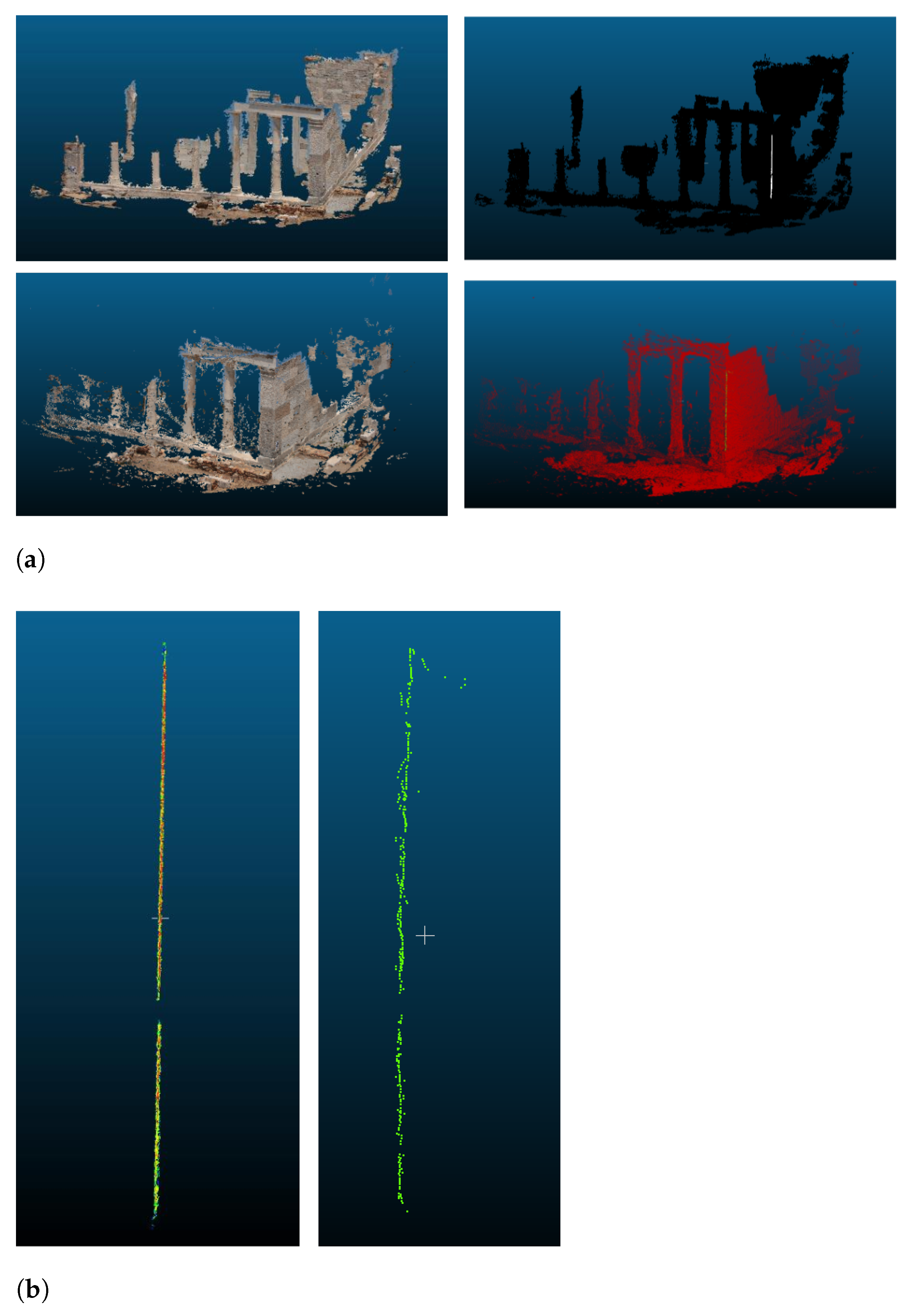
The four-channel images were imported in both professional SfM-MVS software and so the semantically enriched 3D point clouds were created (Figure 8a). The first row of Figure 8a depicts the semantically enriched point cloud produced using the Agisoft-Metashape software while the second row is the semantically enriched point cloud produced using the modified Mapillary-OpenSfM software. Each row in Figure 8a depicts exactly the same 3D point cloud, the difference is due to the semantic knowledge which is carried into the 3D point-cloud file simultaneously with the RGB colors; it is possible to change the color and so visualize the semantic information instead of the true-colors point cloud. The white line in the black point cloud of the first row (Agisoft-Metashape) can be observed, as well as the green line in the red point cloud of the second row (Mapillary-OpenSfM) of Figure 8a. The visualization was made using Cloud Compare, and the colors changed from true colors to semantic colors, by selecting scalar index instead of RGB. Previously, the scalar index was associated with the labels of the point-cloud file. Afterwards, as is described in Section 3, the 3D points were classified into edge and non-edge points. Figure 8b depicts the 3D edge points detected using Agisoft-Metashape (left) and Mapillary-OpenSfM (right) software.
4.3. Implementation of the 3DPlan Software
The proposed algorithm (3DPlan) is divided into three sections: (i) the user interface, (ii) the environment setting and (iii) the execution of the developed approaches according to the user’s choices. In fact, it is impossible to produce manually annotated edges like Figure 7 for all the edges and all the images of a dataset and so automated methods were included. To be more specific, the 3DPlan algorithm includes the live-Canny implementation (Figure 2), which gives the opportunity to the user to set and evaluate simultaneously the Canny’s parameters, as well as the “external source” option which gives the opportunity to the user to exploit any 2D edge-detection method. Moreover, 3DPlan software includes the developed algorithm, which enriches the given RGB images with the corresponding edge map as a fourth channel. Additionally, it includes the developed combination of the DBSCAN and RANSAC algorithms, to group the detected edge points into sets of points belonging to each edge and the algorithm which uses the detected group of 3D points, vectorizes them and saves the 3D vectors to a “.dxf” file.
3DPlan User Interface
The 3DPlan algorithm user interface includes a series of questions which are posed to the user at the terminal/command line as well as several informative messages during the execution of the software, e.g., date/time and execution progress. The user must select which method they prefer, answering some questions (Figure 9). It should be mentioned that the user interface was implemented with a defensive perspective, providing a set of useful functions such as the “message”, “error message” and “input check”, handling the entire process. For instance, Figure 9 depicts a false answer (red circle), and the response of the 3DPlan algorithm (red rectangle). First and foremost, the user defines the number of the channels of the input images (three or four) into the SfM-MVS workflow. Secondly, the user selects the approach that will be executed to create the semantically enriched point cloud. The choices provided are the (i) Agisoft-Metashape, (ii) Mapillary-OpenSfM and the (iii) Triangulation. The Agisoft-Metashape approach contains the (i) Python and (ii) GUI implementation and so the user must select which one will be used during the process. Regardless of the selected point-cloud production approach, the 3DPlan algorithm creates a new folder called “Lines” in the 3DPlan directory. Thirdly, the user selects the approach which will be used to determine the edge semantic information, the first choice is the (i) live-Canny and the second one is the (ii) external semantic source. Finally, the user must define the format of the given three-channel images which will be used to produce the four-channel images. The next steps are executed depending on the selected algorithm, which will be used to produce the semantically enriched point cloud (Figure 3).
4.4. The Environment Setting and the Execution of the Algorithm
Simultaneously to the user’s responses to the interface, the 3DPlan algorithm constructs the environment within which the algorithm will be executed according to the user choices, e.g., it creates the directory in which the final product will be stored, or manipulates the OpenSfM software by creating new folders, copying the four-channel images to the expected from the algorithm folder inside the OpenSfM installation and executing the terminal commands in order to use OpenSfM algorithms, etc. The OpenSfM installation and the 3DPlan software must be in the same folder (“parent directory” in Figure 10). The general folders’ structure is depicted in Figure 10. The three-channel images, i.e., the given dataset, is stored into the “rgb” folder; the “lib” folder contains the Python source code. When the four-channel images are created, they are stored into the “Images” folder. The semantically enriched 3D point cloud, as well as the 3D edge points and the 3D vectors, are stored in the “Lines” folder. In case of already-produced 2D edge maps, these are stored into the “semantic_images” folder to be exploited by the 3DPlan algorithm and, finally, to create the four-channel images. The “Labels” and “Blur_rgb” folders are used for optional debugging/monitoring purposes.
The steps of the proposed approach are presented in Section 3 and Figure 3. The experiments were conducted using the 3DPlan software in combination with several RGB images from (i) the Ancient Temple of Demeter and (ii) the Old Police Station in Monolithos, Rhodes, datasets. The results are depicted in Figure 11a–d and Figure 12a–d.
5. Discussion
The proposed approach has individual steps which should be evaluated separately. The main scope of this effort was the detection of the 3D edges into the produced point cloud using 2D edge semantic information. In fact, the quality of the detection of the 3D edges, using the 3DPlan algorithm, is inextricably linked to the quality of the detection of the 2D edges. The proposed algorithm contains a live-Canny implementation in which the user handles Canny drawbacks, such as misdetections due to textured areas or the shadows present. Additionally, the 3DPlan algorithm includes a blurring implementation using a Gaussian kernel, which, in combination with the live-Canny, produces better results, although misdetections and wrong eliminations are not completely confronted. In general, a plethora of traditional and modern 2D edge-detection approaches are presented in the literature. Thus, the 3DPlan algorithm offers the user the opportunity to exploit any 2D edge-detection method easily and effectively using the “external semantic source” choice. To be more specific, the user can produce images’ edge maps using a technique of his choice and then save them into the “semantic images" directory. The 3DPlan algorithm will enrich the given RGB images with their edge maps included in the “semantic images" directory; hence, the 3DPlan algorithm can be easily combined with all the existing and upcoming 2D edge-detection techniques, thus following the evolution of such techniques. The main contributions of the 3DPlan algorithm are:
- The creation of four-channel images using the given RGB images and their label channel.
- The creation of a semantically enriched point cloud exploiting the four-channel images in combination with professional SfM-MVS software.
- The modification of the Mapillary-OpenSfM software in order to create semantically enriched point clouds using four-channel images.
- The detection of the 3D edges with the most feasible accuracy with respect to the quality of the 2D edge semantic information.
- A software, which is available on GitHub (https://github.com/thobet/3DPlan (accessed on 15 September 2022)) and could be used as a base for more sophisticated approaches to the automation of the production of 2D–3D architectural drawings.
5.1. Creation of Four-Channel Images
The combination of the RGB images with their label channel for the production of the RGBL images was evaluated. To be more precise, after the generation of the RGBL images, they were decomposed into their channels, i.e., R, G, B and L. The primary channels, i.e., R, G and B, were combined and saved while the L channel was saved separately. The initial RGB images were compared with the new RGB images by subtracting from each other and no differences were observed. Hence, it was concluded that the RGB images were unaffected during the process of adding the extra L channel. Apart from the RGB images, the same comparison was performed for the label channels. The described procedure is illustrated in Figure 13.
5.2. Classification of 3D Points into Edge and Non-Edge Points
Apart from the quality of the 2D edge-detection technique, the classification of the 3D points into edge and non-edge points contributes to the detection of the 3D edge points with the best possible accuracy. During the classification procedure, the label value of each point is taken into account to classify it as an edge or non-edge point. Ideally, the label values must be either 0 or 255, representing the non-edge and edge points, respectively. The generated label values, using the Agisoft-Metashape and the modified Mapillary-OpenSfM workflows, rang between 0 and 255 because the images are resized during the execution of the SfM-MVS pipelines to reduce the computational cost of the algorithms. Additionally, some 2D edges were not detected in all the images in which they are depicted, due to the weaknesses of the performed 2D edge-detection technique and so the mean value of the pixels associated with the 3D point is not equal to 255. To this end, a threshold value, which is used as an empirical classification criterion, was included into the 3DPlan algorithm. The idea is that the 3D points with values larger than the threshold constitute the “strong” edge points in contrast to those with values smaller than the threshold, which constitute the “weak” edge points. The label value of the non-edge points is equal to zero. This process filters the detected edge points and stores the “strong” ones. The remaining edge points using a classification criterion equal to 0, 100, 150 and 200, respectively, are depicted in Figure 14.
5.3. 3D Edge Points of Each Edge and 3D Vectorization
Afterwards, the “strong” edge points are fed into the DBSCAN algorithm, which aims to decompose the detected points into clusters presenting the points of each edge. Two variables are defined, i.e., the “min samples” and the “eps”. The “min samples” sets the minimum number of points required into a cluster to be validated and defined as a value larger than two to eliminate sets of clusters, which are more likely to be erroneous because the clusters with small number of points describe areas with a sparsity of 3D points, and, thus, are considered as noise. The “eps” value defines each point’s neighborhood and so it must be smaller than the average distance between the 3D points in order to separate them efficiently, into points of each 3D edge. Afterwards, the points of each edge are imported into the RANSAC algorithm, in which the inliers are considered using line fitting and used into the 3D vectorization step. The results of the combination of the DBSCAN and RANSAC algorithms as well as the 3D vectorization step need further investigation (Figure 11c,d and Figure 12c,d). In this effort, the 3D vectorization procedure is conducted using the first and the last point of each cluster produced using the RANSAC algorithm; this procedure must be changed in order to exploit the information of each point into the cluster to fit the most accurate 3D line. To this end, the parameters calculated from the RANSAC algorithm could be exploited during the vectorization step. Moreover, different clustering algorithms and statistical methods could be applied to future implementations to separate the 3D points into points of each edge. Additionally, different implementations using the provided algorithms (DBSCAN and RANSAC) must be performed to investigate their performance using several combinations of their parameters. The clustering and 3D vectorization tasks constitute a first investigation of the problem and, obviously, further analysis is essential.
5.4. 3D Point-Cloud Characteristics and Post-Processing
The characteristics of the created 3D point cloud play a significant role in the product’s quality and, thus, the performance of the SfM-MVS workflows is vital. More concretely, a point cloud with reduced noise, dense distribution of points and without a lack of information constitute a high-quality product and so the 3DPlan algorithm could detect and separate the 3D edges with the most feasible accuracy. To this end, the 3DPlan algorithm was linked with the Agisoft-Metashape and the modified Mapillary-OpenSfM software. The semantic information is passed to the semantically enriched point cloud, exploiting the professional software and the four-channel images. Figure 11a,b and Figure 12a,b depict the semantic information passed to the 3D space correctly, with respect to the label channels. In addition to the professional SfM-MVS software, the 3DPlan algorithm includes the “Triangulation” algorithm. The “Triangulation" algorithm is not an accurate and recommended approach for the 3D edge-detection task, after all, the scope of that algorithm was the development of the secondary Python scripts and not the production of a professional SfM-MVS software. Apart from the generation of the point cloud, a post process of it, e.g., removing the ground points or the blue points coming from sky, etc., could improve the 3D edge-detection task. Several experiments using a post-processed point cloud could be performed to validate the performance of the 3DPlan algorithm using high-quality point clouds. In addition, software performance and the complexity of the object under investigation affect the quality of the product. For instance, the Old Police Station dataset, which is built of stones, presents several misdetections because stones’ edges are similar to noise and, thus, are eliminated during the process (Figure 15). Additionally, the stones are characterized by textured areas and shadows, which make the edge-detection procedure difficult. Hence, a plethora of experiments using different threshold values should be conducted in each case study, during the execution of the 3DPlan algorithm, to find the optimal parameters and so the most accurate result. Finally, the modified Mapillary-OpenSfM approach is available only for the Ubuntu distribution while the Agisoft-Metashape approach is available for any operating system and so the 3DPlan algorithm can be executed using every operating system. The Mapillary-OpenSfM is a non-commercial software and, thus, the 3DPlan algorithm can be used by everyone. Additionally, during the execution of the 3DPlan algorithm, no extra mathematical equations are included, apart from those used from the SfM-MVS software and, thus, additional errors are not embedded.
6. Concluding Remarks and Future Work
In this effort, an open-source 3D edge-detection and vectorization algorithm written in Python is presented. To be more specific, the RGB images, which are used for the point-cloud production, are enriched with an extra channel, which contains the edge semantic information. Afterwards, professional SfM-MVS pipelines are exploited to produce the semantically enriched point cloud. In fact, the 3DPlan algorithm works with point clouds produced by the SfM-MVS process only. Eventually, the 3D edge points are firstly separated and then classified into the points of each edge. Each cluster is passed into the vectorization step from which the 3D vectors are created and saved using the “.dxf” format. The 3DPlan software can be combined with any 2D edge-detection technique as well as with any 2D image-segmentation technique, e.g., semantic segmentation, instance segmentation, panoptic segmentation etc., to pass the label channel information into 3D space. Additionally, it uses professional and guaranteed SfM-MVS software (Agisoft-Metashape and Mapillary-OpenSfM) for the generation of the semantically enriched point cloud. Apart from that, during the execution of the 3DPlan algorithm, extra mathematical equations are not included, such as plane intersection, and, thus, additional errors are not embedded to the 3D edge-detection process. On the other hand, the clustering approach, i.e., the combination of the DBSCAN and RANSAC algorithms, suffers from several erroneously detected clusters. Apart from that, the 3D vectorization procedure is over-simplified without the exploitation of the entire information of each cluster, i.e., every detected 3D edge point, and, thus, a further investigation and development of those methods is required. The presented results contain too many artifacts and the output drawings contain too many vectors, due to the aforementioned disadvantages, so except from the improvement of the existing steps, simplification and topology analysis steps should be included in 3DPlan software. Additionally, a GUI of the 3DPlan software could be produced in order to be convenient for a plethora of users. The detected edges using a georeferenced point cloud and the 3DPlan software can be compared with the real edges captured by conventional surveying methods (total station) to evaluate the precision of the process. More precisely, we could measure a specific edge using a total station, then digitally measure the same edge detected by the 3DPlan algorithm and, finally, subtract one from the other to evaluate the precision of the detected 3D edge. In fact, the evaluation should be conducted for a large number of specific edges, to draw accurate conclusions. In Section 2, some methods which exploit BIM models are presented. The creation of a detailed BIM is difficult especially into the cultural-heritage domain, which is characterized by complexity and heterogeneity. In Section 2, edge-detection methods are investigated more than methods using BIM because the proposed approach investigates a simple yet efficient pipeline to detect 3D edges exploiting 2D edge semantic information in combination with professional SfM-MVS software. Additionally, the poor 2D edge semantic information is one of the major reasons for the detection of erroneous 3D edge points by the 3DPlan software and, thus, an improved 2D edge-detection procedure would produce better edge semantic information to feed into the 3DPlan software. Moreover, a comparison between the traditional and deep-learning 2D edge-detection approaches should be conducted to find the most suitable one for the automation of the production of architectural vector drawings. An investigation of the efficiency of the 3DPlan software applied to objects with several characteristics such as complexity, size, etc., could be also conducted. Furthermore, another interesting investigation could be the implementation of the 3DPlan algorithm for the detection of multiple and more complex objects or a detailed semantic segmentation in 3D space. To conclude, the 3DPlan software extracts 3D edges with the most feasible accuracy, depending on the 2D edge-detection technique and can be executed by everyone, in any operating system.
Author Contributions
Conceptualization, A.G.; Methodology, A.G. and T.B.; Software, T.B.; Validation, T.B. and A.G.; Formal analysis, T.B.; Writing—original draft preparation, T.B.; Writing—review and editing, T.B. and A.G.; Supervision, A.G. All authors have read and agreed to the published version of the manuscript.
Funding
This research was partially funded by the General Secretariat of Research and Technology through an EU matching funds project.
Data Availability Statement
The data and material used in this research were provided by the Laboratory of Photogrammetry of NTUA and originate from previous projects. The python code of the 3DPlan software is available on Github [https://github.com/thobet/3DPlan (accessed on 15 September 2022)]. The Python code of the new branch of the Mapillary-OpenSfM software is available on GitHub [https://github.com/thobet/OpenSfM_3DPlan (accessed on 15 September 2022)].
Acknowledgments
The authors would like to thank PhD Candidate in NTUA, Elisavet (Ellie) K. Stathopoulou for her advice during this effort.The Python code is available on GitHub.
Conflicts of Interest
There are no conflicts of interest.
Abbreviations
The following abbreviations are used in this manuscript:
| DBSCAN | Density-based spatial clustering of applications with noise |
| MVS | Multi-view stereo |
| RANSAC | Random sample consensus |
| SfM | Structure from motion |
References
- Murtiyoso, A.; Pellis, E.; Grussenmeyer, P.; Landes, T.; Masiero, A. Towards Semantic Photogrammetry: Generating Semantically Rich Point Clouds from Architectural Close-Range Photogrammetry. Sensors 2022, 22, 966. [Google Scholar] [CrossRef] [PubMed]
- Pellis, E.; Murtiyoso, A.; Masiero, A.; Tucci, G.; Betti, M.; Grussenmeyer, P. An Image-Based Deep Learning Workflow for 3D Heritage Point Cloud Semantic Segmentation. Int. Arch. Photogramm. Remote. Sens. Spat. Inf. Sci.-ISPRS Arch. 2022, 46, 429–434. [Google Scholar] [CrossRef]
- Gülch, E.; Obrock, L. Automated semantic modelling of building interiors from images and derived point clouds based on deep learning methods. Int. Arch. Photogramm. Remote. Sens. Spat. Inf. Sci. 2020, 43, 421–426. [Google Scholar] [CrossRef]
- Stathopoulou, E.K.; Remondino, F. Semantic photogrammetry: Boosting image-based 3D reconstruction with semantic labeling. Int. Arch. Photogramm. Remote. Sens. Spat. Inf. Sci. 2019, 42, W9. [Google Scholar] [CrossRef] [Green Version]
- Stathopoulou, E.K.; Battisti, R.; Cernea, D.; Remondino, F.; Georgopoulos, A. Semantically derived geometric constraints for MVS reconstruction of textureless areas. Remote Sens. 2021, 13, 1053. [Google Scholar] [CrossRef]
- Blake, B. On Draughtsmanship and the 2 & a Half D World. Available online: https://billboyheritagesurvey.wordpress.com/2022/09/23/on-draughtsmanship-and-the-2and-a-half-d-world/ (accessed on 4 October 2022).
- Minaee, S.; Boykov, Y.Y.; Porikli, F.; Plaza, A.J.; Kehtarnavaz, N.; Terzopoulos, D. Image segmentation using deep learning: A survey. IEEE Trans. Pattern Anal. Mach. Intell. 2021, 44, 3523–3542. [Google Scholar] [CrossRef]
- Xie, Y.; Tian, J.; Zhu, X.X. Linking points with labels in 3D: A review of point cloud semantic segmentation. IEEE Geosci. Remote Sens. Mag. 2020, 8, 38–59. [Google Scholar] [CrossRef] [Green Version]
- Zhang, J.; Zhao, X.; Chen, Z.; Lu, Z. A review of deep learning-based semantic segmentation for point cloud. IEEE Access 2019, 7, 179118–179133. [Google Scholar] [CrossRef]
- Agisoft-Metashape. Discover Intelligent Photogrammetry with Metashape. 2016. Available online: http://www.agisoft.com/ (accessed on 4 October 2022).
- Mapillary-OpenSfM. An Open-Source Structure from Motion Library That Lets You Build 3D Models from Images. Available online: https://opensfm.org/ (accessed on 4 October 2022).
- Bienert, A. Vectorization, edge preserving smoothing and dimensioning of profiles in laser scanner point clouds. In Proceedings of the XXIst ISPRS Congress, Beijing, China, 3–11 July 2008; Volume 311. [Google Scholar]
- Nguatem, W.; Drauschke, M.; Mayer, H. Localization of Windows and Doors in 3d Point Clouds of Facades. ISPRS Ann. Photogramm. Remote Sens. Spat. Inf. Sci. 2014, II-3, 87–94. [Google Scholar] [CrossRef] [Green Version]
- Lin, Y.; Wang, C.; Cheng, J.; Chen, B.; Jia, F.; Chen, Z.; Li, J. Line segment extraction for large scale unorganized point clouds. ISPRS J. Photogramm. Remote Sens. 2015, 102, 172–183. [Google Scholar] [CrossRef]
- Grompone von Gioi, R.; Jakubowicz, J.; Morel, J.M.; Randall, G. LSD: A line segment detector. Image Process. Line 2012, 2, 35–55. [Google Scholar] [CrossRef] [Green Version]
- Mitropoulou, A.; Georgopoulos, A. An automated process to detect edges in unorganized point clouds. ISPRS Ann. Photogramm. Remote. Sens. Spat. Inf. Sci. 2019, 4, 99–105. [Google Scholar] [CrossRef] [Green Version]
- PCL. Point Cloud Library. Available online: https://pointcloudlibrary.github.io/ (accessed on 4 October 2022).
- Bazazian, D.; Casas, J.R.; Ruiz-Hidalgo, J. Fast and robust edge extraction in unorganized point clouds. In Proceedings of the 2015 International Conference on Digital Image Computing: Techniques and Applications (DICTA), Adelaide, SA, Australia, 23–25 November 2015; pp. 1–8. [Google Scholar]
- Lu, X.; Liu, Y.; Li, K. Fast 3D line segment detection from unorganized point cloud. arXiv 2019, arXiv:1901.02532. [Google Scholar]
- Dolapsaki, M.M.; Georgopoulos, A. Edge Detection in 3D Point Clouds Using Digital Images. ISPRS Int. J.-Geo-Inf. 2021, 10, 229. [Google Scholar] [CrossRef]
- Alshawabkeh, Y. Linear feature extraction from point cloud using color information. Herit. Sci. 2020, 8, 28. [Google Scholar] [CrossRef]
- Canny, J.F. Finding Edges and Lines in Images; Technical Report; Massachusetts Inst of Tech Cambridge Artificial Intelligence Lab: Cambridge, MA, USA, 1983. [Google Scholar]
- Bao, T.; Zhao, J.; Xu, M. Step edge detection method for 3D point clouds based on 2D range images. Optik 2015, 126, 2706–2710. [Google Scholar] [CrossRef]
- Hofer, M.; Maurer, M.; Bischof, H. Efficient 3D scene abstraction using line segments. Comput. Vis. Image Underst. 2017, 157, 167–178. [Google Scholar] [CrossRef]
- Bazazian, D.; Parés, M.E. EDC-Net: Edge detection capsule network for 3D point clouds. Appl. Sci. 2021, 11, 1833. [Google Scholar] [CrossRef]
- Koch, S.; Matveev, A.; Jiang, Z.; Williams, F.; Artemov, A.; Burnaev, E.; Alexa, M.; Zorin, D.; Panozzo, D. Abc: A big cad model dataset for geometric deep learning. In Proceedings of the IEEE/CVF Conference on Computer Vision and Pattern Recognition, Long Beach, CA, USA, 15–20 June 2019; pp. 9601–9611. [Google Scholar]
- Chang, A.X.; Funkhouser, T.; Guibas, L.; Hanrahan, P.; Huang, Q.; Li, Z.; Savarese, S.; Savva, M.; Song, S.; Su, H. Shapenet: An information-rich 3d model repository. arXiv 2015, arXiv:1512.03012. [Google Scholar]
- Qi, C.R.; Su, H.; Mo, K.; Guibas, L.J. Pointnet: Deep learning on point sets for 3d classification and segmentation. In Proceedings of the IEEE Conference on Computer Vision and Pattern Recognition, Honolulu, HI, USA, 21–26 July 2017; pp. 652–660. [Google Scholar]
- Qi, C.R.; Yi, L.; Su, H.; Guibas, L.J. PointNet++: Deep Hierarchical Feature Learning on Point Sets in a Metric Space. arXiv 2018, arXiv:1706.02413. [Google Scholar]
- Liu, Y.; D’Aronco, S.; Schindler, K.; Wegner, J.D. PC2WF: 3D Wireframe Reconstruction from Raw Point Clouds. arXiv 2021, arXiv:2103.02766. [Google Scholar]
- Chuang, T.Y.; Sung, C.C. Learning-guided point cloud vectorization for building component modeling. Autom. Constr. 2021, 132, 103978. [Google Scholar] [CrossRef]
- Bassier, M.; Vergauwen, M.; Van Genechten, B. Automated Semantic Labelling of 3D Vector Models for Scan-to-BIM. In Proceedings of the 4th Annual International Conference on Architecture and Civil Engineering (ACE 2016), Singapore, 25–26 April 2016. [Google Scholar] [CrossRef]
- Macher, H.; Landes, T.; Grussenmeyer, P. From Point Clouds to Building Information Models: 3D Semi-Automatic Reconstruction of Indoors of Existing Buildings. Appl. Sci. 2017, 7, 1030. [Google Scholar] [CrossRef]
- Ochmann, S.; Vock, R.; Klein, R. Automatic reconstruction of fully volumetric 3D building models from oriented point clouds. ISPRS J. Photogramm. Remote. Sens. 2019, 151, 251–262. [Google Scholar] [CrossRef] [Green Version]
- Obrock, L.S.; Gülch, E. First steps to automated interior reconstruction from semantically enriched point clouds and imagery. Int. Arch. Photogramm. Remote Sens. Spat. Inf. Sci. 2018, XLII-2, 781–787. [Google Scholar] [CrossRef] [Green Version]
- Chen, L.C.; Zhu, Y.; Papandreou, G.; Schroff, F.; Adam, H. Encoder-decoder with atrous separable convolution for semantic image segmentation. In Proceedings of the European conference on computer vision (ECCV), Munich, Germany, 8–14 September 2018; pp. 801–818. [Google Scholar]
- Long, J.; Shelhamer, E.; Darrell, T. Fully convolutional networks for semantic segmentation. In Proceedings of the IEEE Conference on Computer Vision and Pattern Recognition, Boston, MA, USA, 7–12 June 2015; pp. 3431–3440. [Google Scholar]
- Xie, S.; Tu, Z. Holistically-nested edge detection. In Proceedings of the IEEE International Conference on Computer Vision, Washington, DC, USA, 7–13 December 2015; pp. 1395–1403. [Google Scholar]
- Poma, X.S.; Riba, E.; Sappa, A. Dense extreme inception network: Towards a robust cnn model for edge detection. In Proceedings of the IEEE/CVF Winter Conference on Applications of Computer Vision, Waikoloa, HI, USA, 4–8 January 2020; pp. 1923–1932. [Google Scholar]
- He, J.; Zhang, S.; Yang, M.; Shan, Y.; Huang, T. Bi-directional cascade network for perceptual edge detection. In Proceedings of the IEEE/CVF Conference on Computer Vision and Pattern Recognition, Long Beach, CA, USA, 15–20 June 2019; pp. 3828–3837. [Google Scholar]
- Liu, Y.; Cheng, M.M.; Hu, X.; Wang, K.; Bai, X. Richer convolutional features for edge detection. In Proceedings of the IEEE Conference on Computer Vision and Pattern Recognition, Honolulu, HI, USA, 21–26 July 2017; pp. 3000–3009. [Google Scholar]
- Wang, Y.; Zhao, X.; Huang, K. Deep crisp boundaries. In Proceedings of the IEEE Conference on Computer Vision and Pattern Recognition, Honolulu, HI, USA, 21–26 July 2017; pp. 3892–3900. [Google Scholar]
- Bhanu, B.; Lee, S.; Ho, C.C.; Henderson, T. Range data processing: Representation of surfaces by edges. In Proceedings of the Eighth International Conference on Pattern Recognition, Paris, France, 21–31 October 1986; IEEE Computer Society Press: Piscataway, NJ, USA, 1986; pp. 236–238. [Google Scholar]
- The 3-Clause BSD License | Open Source Initiative. Available online: https://opensource.org/licenses/BSD-3-Clause (accessed on 4 October 2022).
- Fischler, M.A.; Bolles, R.C. Random sample consensus: A paradigm for model fitting with applications to image analysis and automated cartography. Commun. ACM 1981, 24, 381–395. [Google Scholar] [CrossRef]
- Bolles, R.C.; Fischler, M.A. A RANSAC-based approach to model fitting and its application to finding cylinders in range data. In Proceedings of the IJCAI, Vancouver, BC, Canada, 24–28 August 1981; Volume 1981, pp. 637–643. [Google Scholar]
- Ester, M.; Kriegel, H.P.; Sander, J.; Xu, X. A density-based algorithm for discovering clusters in large spatial databases with noise. In Proceedings of the kdd, Portland, OR, USA, 2–4 August 1996; Volume 96, pp. 226–231. [Google Scholar]
- OpenCV. Open Source Computer Vision Library. Available online: https://opencv.org/ (accessed on 4 October 2022).
- Stefanakis, M.; Kalogeropoulos, K.; Georgopoulos, A.; Bourbou, C. Exploring the ancient demos of Kymissaleis on Rhodes: Multdisciplinary experimental research and theoretical issues. In Classical Archaeology in Context: Theory and Practice in Excavation in the Greek World; Walter de Gruyter GmbH & Co. KG: Berlin, Germany, 2015; pp. 259–314. [Google Scholar]
- Stefanakis, M.I. The Kymissala (Rhodes, Greece) Archaeological Research Project. Archeologia 2015, 66, 47–63. [Google Scholar]
- Georgopoulos, A.; Tapinaki, S.; Stefanakis, M.I. Innovative Methods for Digital Heritage Documentation: The archaeological site of Kymissala in Rhodes. In Proceedings of the ICOMOS 19th General Assembly and Scientific Symposium “Heritage and Democracy”, New Delhi, India, 13–14 December 2017. [Google Scholar]
Figure 1.
General idea of the 3DPlan algorithm. The products from left to right are: the semantically enriched point cloud visualized with true colors, semantic colors, the detected 3D edge and the 3D vector with the dense point cloud.
Figure 1.
General idea of the 3DPlan algorithm. The products from left to right are: the semantically enriched point cloud visualized with true colors, semantic colors, the detected 3D edge and the 3D vector with the dense point cloud.

Figure 2.
Live-Canny interface.

Figure 3.
The flowchart of the 3DPlan software (above to below).

Figure 4.
The image pair and reference image (Experiment 1).

Figure 5.
The semantically enriched point cloud (Experiment 1).

Figure 6.
The edge semantic information (first row); the semantically enriched point cloud using the triangulation algorithm (second row).
Figure 6.
The edge semantic information (first row); the semantically enriched point cloud using the triangulation algorithm (second row).

Figure 7.
Edge semantic information used with professional SfM-MVS software.

Figure 8.
Products using professional SfM-MVS software and manually annotated edges. (a) Semantically enriched dense point clouds using the Agisoft-Metashape (first row) and the Mapillary-OpenSfM software (second row). (b) 3D edge points using the Metashape (left) and the OpenSfM software (right).
Figure 8.
Products using professional SfM-MVS software and manually annotated edges. (a) Semantically enriched dense point clouds using the Agisoft-Metashape (first row) and the Mapillary-OpenSfM software (second row). (b) 3D edge points using the Metashape (left) and the OpenSfM software (right).

Figure 9.
Questions of the 3DPlan user interface.

Figure 10.
The general folders’ structure.

Figure 11.
The proposed approach and the Temple of Demeter in Naxos dataset. (a) The semantically enriched dense point cloud. (b) The detected 3D edges. (c) The detected 3D edge points of each edge (left) and 3D noise points (right). The colors of each class (left) seem to be the same for large regions of the point cloud. In fact, there are not the same colors, but colors with minimal change in color values due to the existence of hundreds of classes. (d) 3D vectors with the sparse point cloud.


Figure 12.
The proposed approach and the Old Police Station dataset. (a) The semantically enriched dense point cloud. (b) The detected 3D edges. (c) The detected 3D edge points of each edge (left) and 3D noise (right). The colors of each class (left) seem to be the same for large regions of the point cloud. In fact, there are not the same colors, but colors with minimal change in color values due to the existence of hundreds of classes. (d) 3D vectors with the sparse point cloud.


Figure 13.
RGBL image check procedure.

Figure 14.
Remaining edge points using threshold value equal to 0, 100, 150, 200, respectively.

Figure 15.
Close view of the 3D edge points (white) and all the rest of the Old Police Station dataset.
Figure 15.
Close view of the 3D edge points (white) and all the rest of the Old Police Station dataset.

Publisher’s Note: MDPI stays neutral with regard to jurisdictional claims in published maps and institutional affiliations. |
© 2022 by the authors. Licensee MDPI, Basel, Switzerland. This article is an open access article distributed under the terms and conditions of the Creative Commons Attribution (CC BY) license (https://creativecommons.org/licenses/by/4.0/).
Share and Cite
MDPI and ACS Style
Betsas, T.; Georgopoulos, A. Point-Cloud Segmentation for 3D Edge Detection and Vectorization. Heritage 2022, 5, 4037-4060. https://doi.org/10.3390/heritage5040208
AMA Style
Betsas T, Georgopoulos A. Point-Cloud Segmentation for 3D Edge Detection and Vectorization. Heritage. 2022; 5(4):4037-4060. https://doi.org/10.3390/heritage5040208
Chicago/Turabian StyleBetsas, Thodoris, and Andreas Georgopoulos. 2022. "Point-Cloud Segmentation for 3D Edge Detection and Vectorization" Heritage 5, no. 4: 4037-4060. https://doi.org/10.3390/heritage5040208