The Effect of Data Transformation on Singular Spectrum Analysis for Forecasting
by
 , , and
Hossein Hassani
1,*,† ,
,
Mohammad Reza Yeganegi
2,†,
Atikur Khan
3,† and
Emmanuel Sirimal Silva
4,† 1
Department of Business & Management, Webster Vienna Private University, 1020 Vienna, Austria
2
Department of Accounting, Islamic Azad University, Central Tehran Branch, Tehran 477893855, Iran
3
Qantares, 97 Broadway, Nedlands 6009 (Perth), Western Australia, Australia
4
Centre for Fashion Business and Innovation Research, Fashion Business School, London College of Fashion, University of the Arts London, London W1G 0BJ, UK
*
Author to whom correspondence should be addressed.
†
These authors contributed equally to this work.
Signals 2020, 1(1), 4-25; https://doi.org/10.3390/signals1010002
Submission received: 14 January 2020
/
Revised: 12 April 2020
/
Accepted: 17 April 2020
/
Published: 7 May 2020
Abstract
:Data transformations are an important tool for improving the accuracy of forecasts from time series models. Historically, the impact of transformations have been evaluated on the forecasting performance of different parametric and nonparametric forecasting models. However, researchers have overlooked the evaluation of this factor in relation to the nonparametric forecasting model of Singular Spectrum Analysis (SSA). In this paper, we focus entirely on the impact of data transformations in the form of standardisation and logarithmic transformations on the forecasting performance of SSA when applied to 100 different datasets with different characteristics. Our findings indicate that data transformations have a significant impact on SSA forecasts at particular sampling frequencies.
1. Introduction
Amidst the emergence of Big Data and Data Mining techniques, forecasting continues to remain an important tool for planning and resource allocation in all industries. Accordingly, researchers, academics, and forecasters alike invest time and resources into methods for improving the accuracy of forecasts from both parametric and nonparametric forecasting models. One approach to improving the accuracy of forecasts is via data transformations prior to fitting time series models. For example, it is noted in [1] that data transformations can simplify the forecasting task, whilst evidence from other research indicates that, in economic analysis, taking logarithms can provide forecast improvements if it results in stabilising the variance of a series [2]. However, studies also indicate that data transformations will not always improve forecasts [3] and that they could complicate time series analysis models [4,5].
In fact, a key challenge for forecasting under data transformation is to transform the data back to its original scale, a process which could result in a forecasting bias [6,7]. Historically, most studies have focused on the impact of data transformations on parametric models such as Regression and Autoregressive Integrated Moving Average (ARIMA) models [8,9]. More recently, authors have resorted to evaluating the impact of data transformations on several other forecasting models [10,11], further highlighting the relevance and importance of the topic. Our interest is focused on the evaluation of the impact of data transformations on a time series analysis and forecasting technique called Singular Spectrum Analysis (SSA).
In brief, the SSA technique is a popular denoising, forecasting, and missing value prediction technique with both univariate and multivariate capabilities [12,13]. Recently, its diverse applications have focused on forecasting solutions for varied industries and fields, from tourism [14,15] and economics [16,17,18] to fashion [19], climate [20,21], and several other sectors [22,23,24]. Regardless of its wide and varied applications, researchers have yet to explore the effect of data transformations on the forecasting performance of this nonparametric forecasting technique. Previously, in [25], the authors evaluated the forecasting performance of the two basic SSA algorithms under different data structures. However, their work did not extend to evaluating the impact of data transformations to provide empirical evidence for future research. Accordingly, through this paper, we aim to contribute to the existing research gap by studying the effects of different data transformation options on the forecasting behaviour of SSA.
Logarithmic transformation is the most commonly used transformation in time series analysis. It has been used to convert multiplicative time series structures to additive structures or to reduce the time series skewness volatility and increase stability [2,26]. The autocorrelation structure in the time series may change under different transformations that may affect the model, and different transformations may result in different specifications for ARIMA models [6,27]. Like ARIMA models, SSA too can be greatly influenced by transformations. For instance, if data transformation makes noise uncorrelated or reduces the complexity of the time series, it can improve SSA performance [21,26]. As data standardisation and logarithmic transformations are the easiest in terms of interpretability and back-transformation to the original scale, we explore the effect of these data transformations on the forecasting performance of SSA.
The remainder of this paper is organised as follows. In Section 2, we provide a detailed exposition of SSA and its recurrent and vector forecasting algorithms. In Section 3, we present data transformation techniques and their effect on forecasting accuracy. Procedures for examining the effect of transformation based on different characteristics of time series are presented in Section 4. In Section 5, we analyse different datasets of varied characteristics and present our results for an evidence-based exploration of the effect of data transformations on SSA forecasts. Finally, we present our concluding remarks in Section 6.
2. SSA Forecasting
There are two different algorithms for forecasting with SSA, namely recurrent forecasting and vector forecasting [12,28]. Those interested in a comparison of the performance of both algorithms are referred to [25]. Both of these forecasting algorithms require that one follows two common steps of SSA, the decomposition and reconstruction of a time series [12,28]. In what follows, we provide a brief description of forecasting processes in SSA.
2.1. Decomposition and Reconstruction of Time Series
In SSA, we embed the time series into a high-dimensional space by constructing a Hankel structured trajectory matrix of the form:
where m is the window length, the lagged vector is the ith column of the trajectory matrix , , and .
The singular value decomposition (SVD) of the trajectory matrix can be expressed as
where is the jth eigenvector of corresponding to the eigenvalue and .
If k is the number of signal components, represents a matrix of signal, and is the matrix of noise. We apply the diagonal averaging procedure to to reconstruct the signal series such that the observed series can be expressed as
where is the less noisy, filtered series. A detailed explanation of decomposition in Equation (3) can be found in [28,29].
To construct the trajectory matrix in Equation (1) and to conduct the SVD in Equation (2), we have to select the Window Length m and the number of signal components k. Since our aim is not to demonstrate the selection of SSA choices (m and k), we opt not to reproduce the selection procedures for SSA choices, as these are already covered in depth in [12,28]. As our interest is in examining the effect of transformation on the forecasting performance of SSA, we select m and k such that the Root Mean Squared Error (RMSE) in forecasting is minimised.
2.2. Recurrent Forecasting
Recurrent forecasting in SSA is also known as R-forecasting, and the findings in [25] indicate that R-forecasting is best when dealing with large samples. If is the vector of the first elements of the jth eigenvector , and is the last element of . The coefficients of linear recurrent equation can be estimated as
With the parameters in Equation (4), a linear recurrent equation of the form
is used to obtain a one-step-ahead recursive forecast [29]. This linear recurrent formula in Equation (5) is used to forecast the signal at time given the signal at time [28] (Section 2.1, Equations (1)–(6)), and the one-step-ahead recursive forecast of is
We apply the recursive forecasting method in Equation (6) to obtain a one-step-ahead forecast.
2.3. Vector Forecasting
In contrast, the SSA Vector forecasting algorithm has proven to be more robust than the R-forecasting algorithm in most cases [25]. Let us define as the matrix consisting of the first elements of k eigenvectors. The vector forecasting algorithm computes lagged vectors and constructs a trajectory matrix such that
where is the ith column of the reconstructed signal matrix , and is the last elements of the vector .
After a diagonal averaging of the matrix constructed by employing Equation (7), we obtain a time series , as has also been explained in [28] (Section 2.3). Thus, produces a forecast corresponding to for .
3. Transformation of Time Series
Data transformation is useful when the variation increases or decreases with the level of the series [1]. Whilst logarithmic transformation and standardisation are the most commonly used data transformation techniques in time series analysis, it is noteworthy that there are other transformations from the family of power transformation such as square root and cube root transformations. However, the interpretability is not as simple and common as that for standardisation and logarithmic transformation.
3.1. Standardisation
Standardisation of time series is formulated as
where and are the mean and standard deviation of the series , respectively. Data standardisation is another common data transformation in preprocessing. Standardisation is mostly common in machine learning techniques to reduce training time and error. In time series forecasting, standardisation has proven advantages when we are using machine learning algorithms (e.g., neural networks and deep neural networks) [30]. In terms of SSA, the theoretical literature does not investigate the effect of standardisation on SSA forecasts in detail. However, in Golyandina and Zhigljavski [26], the authors addressed the effect of centering the time series as preprocessing. In theory, if the time series can be expressed as an oscillation around a linear trend, centering will increase the SSA’s accuracy [26].
3.2. Logarithmic Transformation
In this paper, the following logarithmic transformation is applied on time series :
where C is a constant value, large enough to guarantee that the term inside the logarithm is positive. As mentioned before, log-transform is a common preprocessing to handle variance instability or right skewness. Furthermore, one may use log-transform as a form of preprocessing to convert a time series with a multiplicative structure to an additive one. Given that SSA can be applied to time series with both additive and multiplicative structures, it does not necessarily need log-transform pre-processing [26]. However, the authors in Golyandina and Zhigljavski [26] showed that using log-transform could affect SSA’s forecasting accuracy. In fact, SSA’s forecasting accuracy will increase if the rank of a transformed series is smaller than the original one.
4. Comparison between Transformations
Time series with different characteristics will behave differently after transformation. For instance, forecasting accuracy in time series, with positive skewness, non-stationarity, and non-normality, may improve with logarithmic transformation. Furthermore, in time series with large observations or large variance, standardisation can improve the forecasting accuracy. Sampling frequency is another potential factor affecting forecasting accuracy. Time series with high sampling frequency (e.g., hourly or daily) usually have an oscillation frequency close to its noise frequency and consequently show instable and noisy behaviour. On the other hand, time series with larger sampling frequency are smoother. These characteristics of time series may affect forecasting and accuracy as well. As such, to investigate the practical effect of data transformation in SSA forecasting, we should consider “Sampling Frequency,” “Skewness,” “Normality,” and “Stationarity” as control factors.
To observe the effectiveness of data transformation prior to the application of SSA, we may compare the forecasting performance of SSA under different transformations and control factors: firstly, by comparing the Root Mean Squared Forecast Error (RMSFE), and secondly, by employing a nonparametric test to examine the treatment effect (data transformation).
4.1. Root Mean Squared Forecast Error (RMSFE)
The most commonly adopted approach for comparing the predictive accuracy between forecasts is to compute and compare the RMSFE from out of sample forecasts. The RMSFE can be defined as
where h is the forecast horizon, N is the number of observations, is observed value of time series, and is the forecasted value.
The application of data transformation prior to forecasting with SSA may significantly affect the forecasting outcome and the affect may vary based on the properties of a time series. Thus, we need to examine the effect of data transformation on RMSFE along with the differing properties of time series. Comparisons between the RMSFE of the original and transformed time series can be used to learn about the forecasting performance of a model for a given time series. However, comparison of RMSFE for a pool of time series with different characteristics is not straightforward. We compute for ( for a short-term forecast, for a long-term forecast, and as a medium-term forecasting horizon) for each of the time series in the pool and examine the effect of transformation by using statistical tests.
4.2. Nonparametric Repeated Measure Factorial Test
Treatment effects in the presence of factors can be examined by employing the nonparametric repeated measure factorial test [31,32] for a pool of time series of different characteristics. Thus, the effect of data transformation (treatment) can be examined by using this test under different characteristics of a time series.
Let us assume that we have K time series in the pool with series code and for each of the series for are computed. If the interest lies on exploring the effect of transformation for the skewness property of time series, we essentially perform the test for treatment effect (transformation) for categories of skewness properties of these time series. There are three factor levels of the factor Skewness, namely Skew Negative, Skew Positive, and Skew Symmetric. Similarly, we will have two levels for the factor Normality (Yes = normal; No = not normal) and two levels for the factor Stationarity (Yes = stationary; No = nonstationary). To test the effect of transformation (No transformation, Standardisation, and Logarithmic transformation), we follow the procedures described below.
First, we learn some basic characteristics of a time series such as normality, stationarity, skewness, and frequency. For example, the frequency of a time series can be learnt by examining the time of measurement: hourly, daily, weekly, monthly, or annually. We also classify time series into different categories via a series of statistical tests such as the Jarque-Bera test for normality [33], the KPSS test for stationarity [34], and the D’Agostino test for skewness [35].
5. Data Analysis
We used the same set of time series employed by Ghodsi et al. [25] to test the effect of data transformation on SSA forecasting accuracy, with different characteristics. The dataset contains 100 real time series with different sampling frequencies and stationarity, normality, and skewness characteristics, representing various fields and categories, obtained via the Data Market (http://datamarket.com). Table 1 presents the number of time series with each feature. It is evident that the real data includes data recorded at varying frequencies (annual, monthly, weekly, daily, and hourly) alongside varying distributions (normal distribution, skewed, stationary, and non-stationary). Interestingly, the majority of the data are non-stationary overtime, which resonates with expectations within real-life scenarios.
The name and description of each time series and their codes assigned to improve presentation are presented in Table A1. Table A2 presents descriptive statistics for all time series to enable the reader to obtain a rich understanding of the nature of the real data. This also includes skewness statistics, and results from the normality (Shapiro-Wilk) and stationarity (Augmented Dickey-Fuller) tests. As visible in Table A1, the data comes from different fields such as energy, finance, health, tourism, housing market, crime, agriculture, economics, chemistry, ecology, and production.
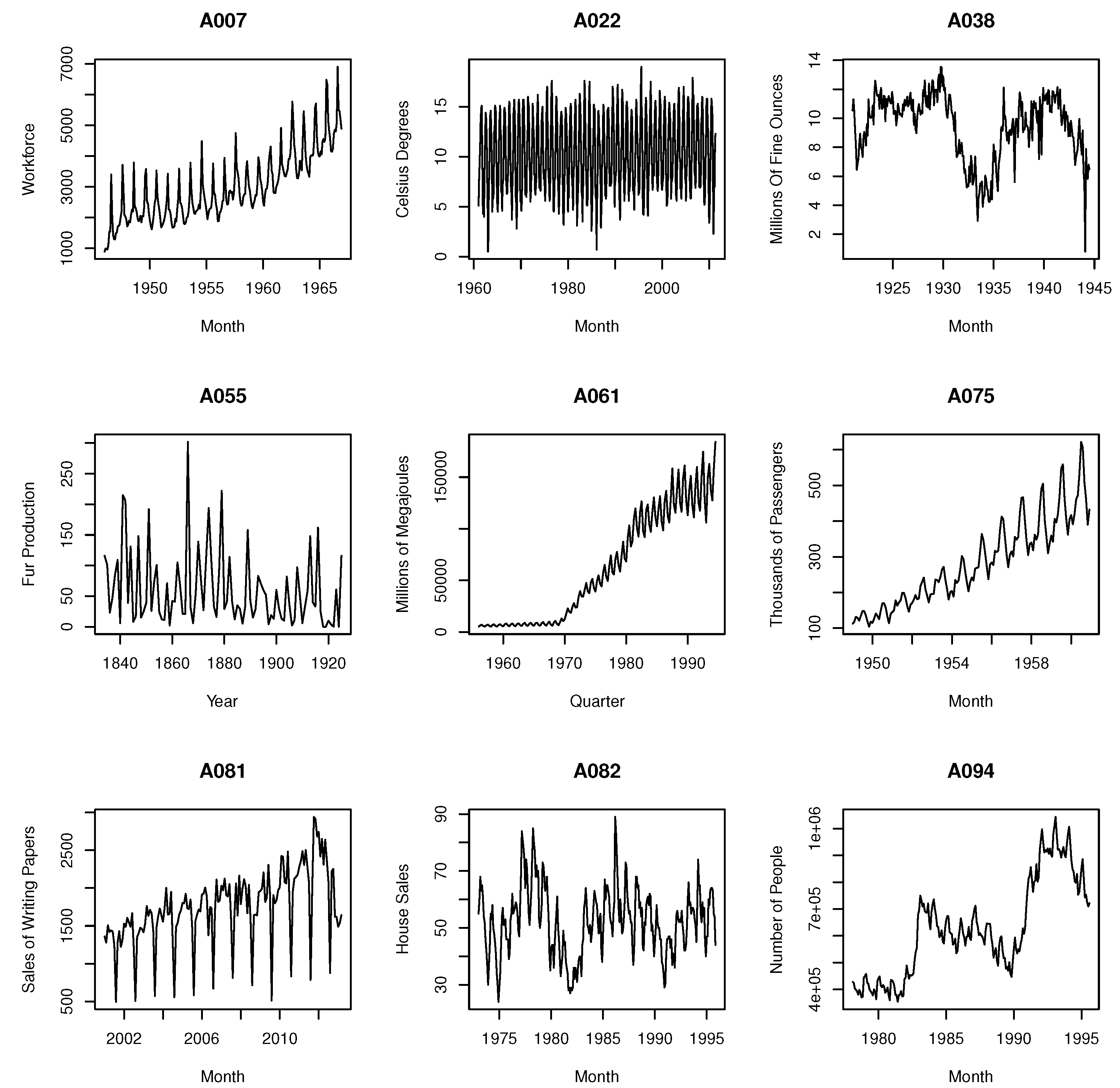
Figure 1 shows the time series for a selection of 9/100 series used in this study. This enables the reader to obtain a further understanding of the different structures underlying the data considered in the analysis. For example, A007 is representative of an asymmetric non-stationary time series for the labour market in a U.S. county. This monthly series shows seasonality with an increasing non-linear trend. In contrast, A022 is related to a meteorological variable that is asymmetric, yet stationary and highly seasonal in nature. An example of a time series that is both asymmetric and non-stationary is A038, which represents the production of silver. Here, structural breaks are visible throughout. A055 is an annual time series, which is stationary and asymmetric, and relates to the production of coloured fox fur. An example of a quarterly time series representing the energy sector is shown via A061. This time series is non-stationary and asymmetric with a non-linear trend and an increasing seasonality over time. Another example focuses on the airline industry (A075) and is also asymmetric and non-stationary in nature. It appears to showcase a linear and increasing trend along with seasonality. A skewed and non-stationary sales series is shown via A081, with the trend indicating increasing seasonality with major drops in the time series between each season. A time series for house sales (A082) can be found to be normally distributed and non-stationary over time. It also shows a slightly curved non-linear trend and a sine wave that is disrupted by noise. Finally, the labour market is drawn on again via A094, but this is an example of a time series affected by several structural breaks leading to a non-stationary, asymmetric series, which also has seasonal periods and a clear non-linear trend.
R packages “Rssa” [36,37,38] and “nparLD” [39] are employed to implement SSA forecasting and the nonparametric repeated measure factorial test, respectively. We apply SSA to three versions of a dataset: a dataset without any transformation, a standardised dataset, and a log-transformed dataset. For each of the three datasets, we obtain RMSFE from out-of-sample forecasting at forecast horizons . It is noteworthy that our aim in this paper is to examine the effect of transformation in SSA forecasting. Thus, we consider the best forecast based on the RMSFE of the last 12 data points regardless of whether the forecast is from the recurrent or vector-based approach.
We also know that the window length m, the number of components k, and the forecasting methods (recurrent and vector) affect the forecasting outcome. Thus, we adopt a computationally intensive approach by considering combinations of m and k, and methods that provide the minimum RMSFE for the out-of-sample forecast for the last 12 data points. The RMSFEs obtained from the computationally intensive approach are given in Table A3, Table A4, Table A5 and Table A6.
Given that the best forecasting results are achieved by util ising a computationally intensive approach, we seek to identify the factors that can affect the RMSFE. In order to address this, we employ statistical tests described in Section 4.2. For each of the series with RMSFE reported in Table A3, Table A4, Table A5 and Table A6, we examine the characteristics of the time series by employing a statistical test, as described in Section 4.2. At this stage, we are ready with the inputs for nonparametric repeated measure factorial test to conduct testing on the treatment effect (data transformation) under different characteristics of these time series. Results obtained from the Wald type tests are provided in Table 2.
Based on the Wald-type test results in Table 2, we may conclude that, at the significance level,
- normality does not affect SSA forecasting performance;
- stationarity affects SSA forecasting performance in long-term forecasting (h = 12) but not at shorter horizons;
- skewness and sampling (observation) frequency affect SSA forecasting performance;
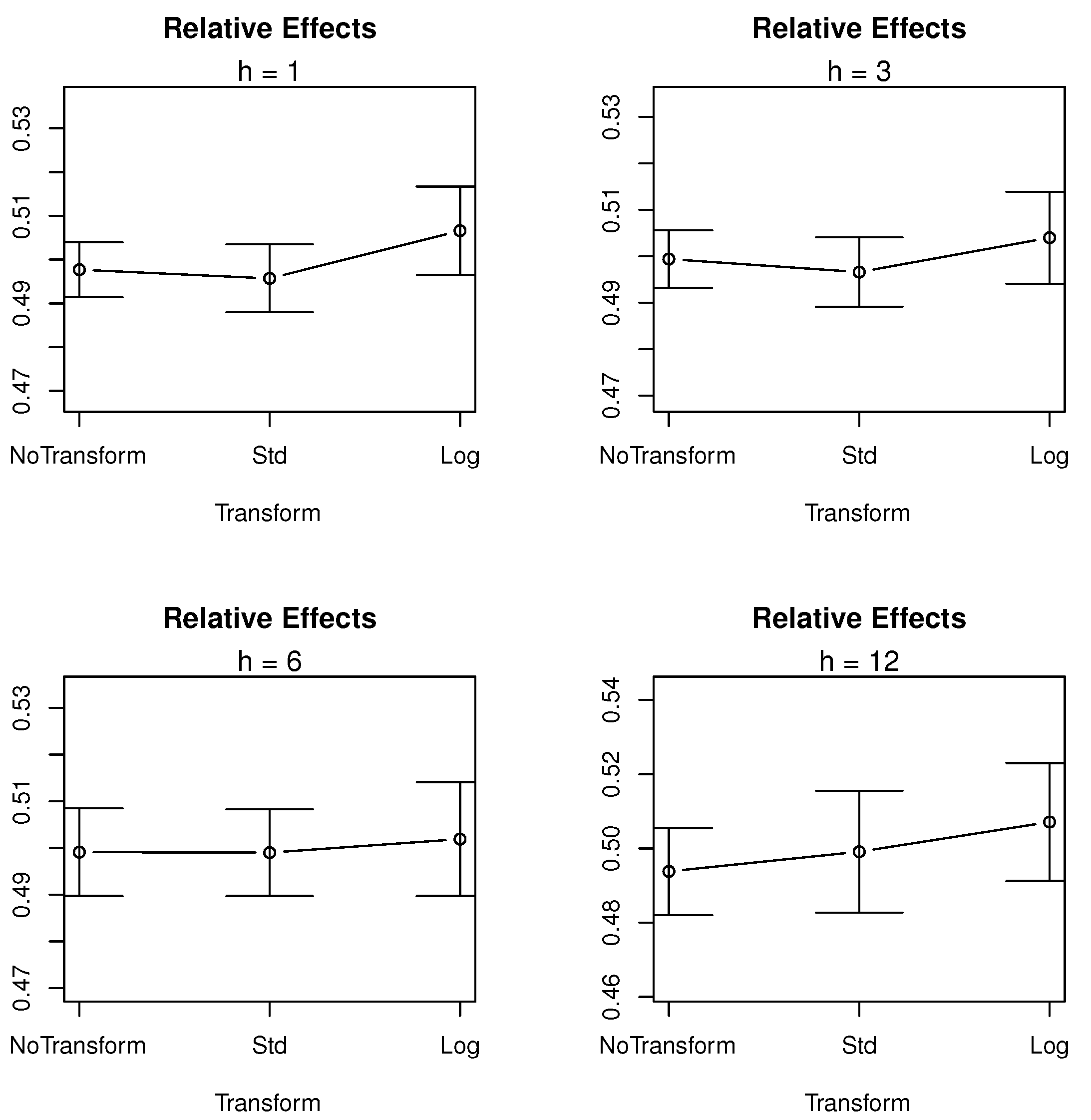
- transformation does not affect SSA forecasting performance, but the interaction between sampling frequencies and transformation is significant, which means the SSA performance is affected by transformation at some sampling frequencies.
The above findings are important in the practice for several reasons. First, in the real world, it is well known that most time series do not meet the assumption of normality. However, as the effect of normality and its interactions with transformations are not significant, when faced with normally distributed data, our findings indicate that there is no impact on the forecasting accuracy of SSA with or without data transformations. Furthermore, these findings also indicate that data transformations do not improve the forecast accuracy in non-normal data either. Secondly, we find that, when series are stationary, it affects the long-term forecasting accuracy of SSA. However, when generating short-term forecasts, the forecasting accuracy of SSA is not affected by stationarity. Thirdly, in reality, as most time series are skewed and increasingly found at varying frequencies (especially following the emergence of Big Data), these findings show that forecasters should remember that varying skewness and frequency of data are features indicative of the need for careful exploration of the use of SSA as the forecasts are sensitive to these features. In general, transformations are not required when forecasting with SSA, as there is no evidence of transformations impacting the SSA forecasting performance; however, there could be a significant impact at certain sampling frequencies. This indicates that, when modelling data with different frequencies, the sensitivity of SSA forecasts to such frequencies could potentially be controlled by transforming the input data.
Since the interaction between sampling frequency and transformation is significant, we explore the relative effect of frequencies on RMSFE. Figure 2 shows the effect plot of treatment (transformation) for different forecast horizons .
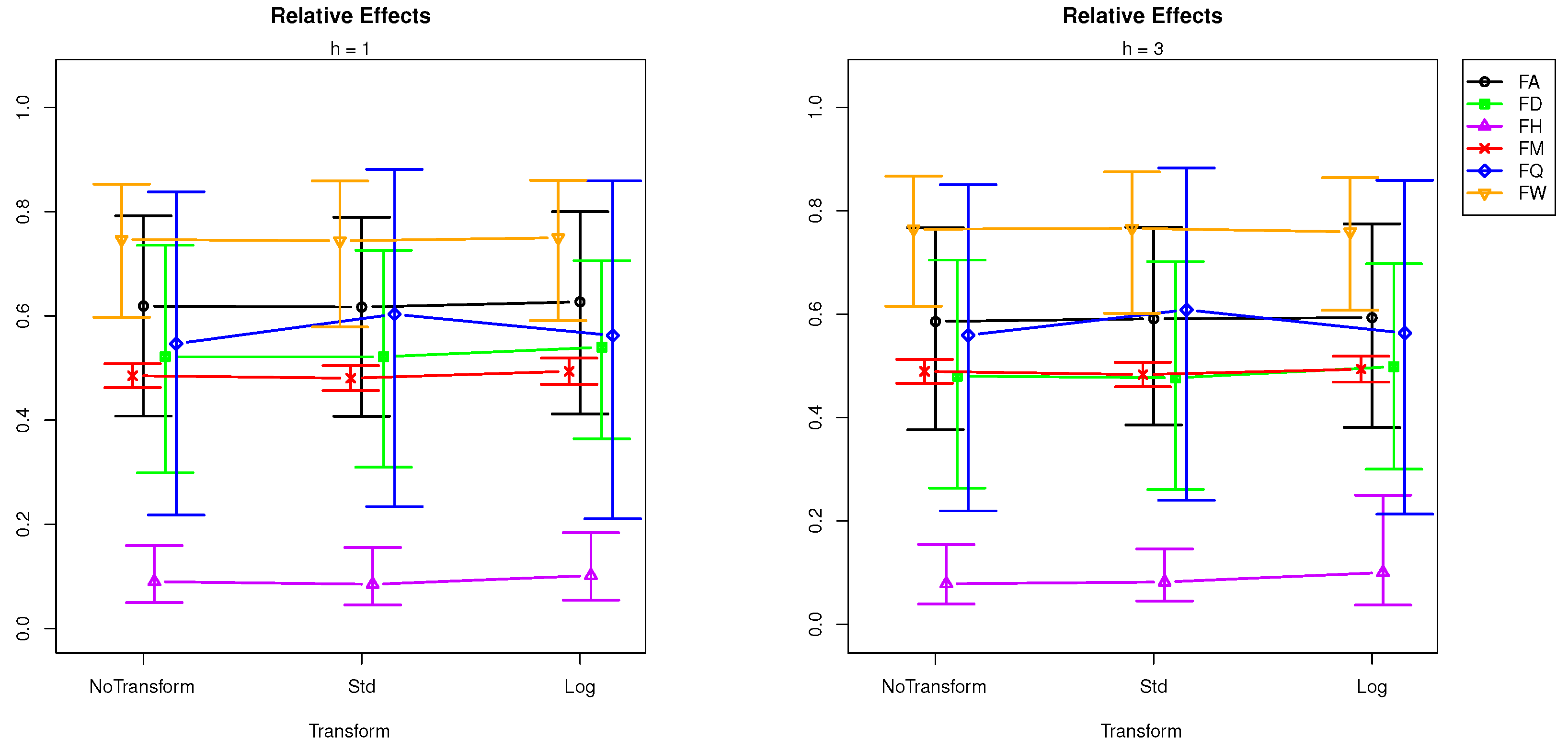
To explore the relative effects of sampling frequency for different forecast horizons, we plot the relative effect of frequencies in Figure 3 and Figure 4.
Sampling frequencies under investigation are hourly (F H), daily (F D), weekly (F W), monthly (F M), and annual (F A). When the relative effect plots in Figure 3 and Figure 4 are compared with the effect plots in Figure 2, we can evaluate how the hourly (F H), weekly (F W), quarterly (F Q), and annual (F A) sampling frequencies are affecting the forecasting performance of SSA. Moreover, the change in shape of the transform’s relative effects (e.g., see the difference between the shapes of “F Q” and “F H” lines in Figure 3 and Figure 4) suggests an interaction between transformation and sampling frequency.
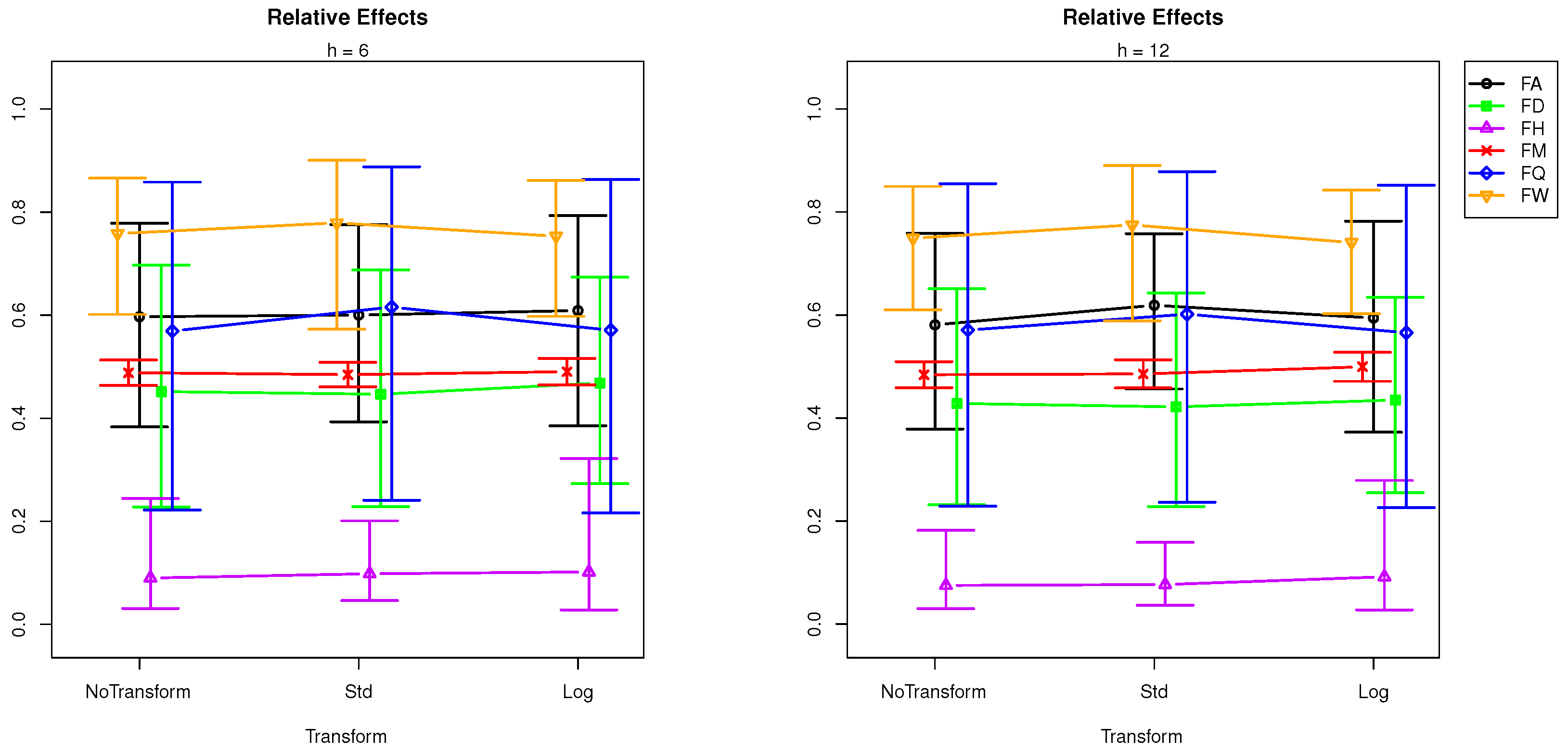
We analyse the results by forecasting horizon. It can be seen in Figure 3 that, in very short-term forecasting (), the standardisation produces a comparatively large RMSFE in quarterly frequencies, while the log transformation reports a slightly larger RMSFE at daily, quarterly, hourly, and annual frequencies. This indicates that users should certainly avoid transforming data with quarterly frequencies when forecasting at step ahead with SSA. In the short-term forecasting horizon () (see Figure 3), the smallest RMSFE belongs to standardisation for monthly frequencies, while standardisation has the largest RMSFE at quarterly frequencies. In mid- and long-term forecasting horizons ( and 12), which are visible in Figure 4, the following can be seen. At steps ahead, standardisation produces the lowest RMSFE at monthly sampling frequencies, whilst it has the largest RMSFE in quarterly and weekly time series data. The log transformation produces higher RMSFEs at daily, hourly, and annual frequencies. Accordingly, the only instance when standardisation could produce better forecasts with SSA at this horizon is when faced with monthly data. At steps ahead, standardisation leads to better forecasts at daily frequencies, whilst log transformations can provide better forecasts with SSA at weekly frequencies.
Finally, these findings indicate that standardisation should only be used to transform data when forecasting with SSA at steps ahead at the daily frequency, at or steps ahead when dealing with a monthly frequency, and at step ahead when forecasting data with monthly or weekly frequencies. At the same time, standardisation should not be employed when forecasting quarterly data at any frequency, as it worsens the forecasting accuracy by comparatively larger margins. Interestingly, log transformations are only suggested when dealing with forecasting weekly data at or steps ahead. In the majority of the instances, SSA is able to provide superior forecasts without the need for data transformations when compared with time series following varied frequencies.
6. Concluding Remarks
This paper focused on evaluating the impact of data transformations on the forecasting performance of SSA, a nonparametric filtering and forecasting technique. Following a concise introduction, the paper introduces the SSA forecasting approaches followed by the transformation techniques considered here. Regardless of its popularity (and in contrast to other methods such as ARIMA and neural networks), there has been no empirical attempt to quantify the impact of data transformations on the forecasting capabilities of SSA. Accordingly, we consider the impact of standardisation and logarithmic transformations on the forecasting performance of both vector and recurrent forecasting in SSA. In order to ensure robustness within the analysis, we not only compare the forecasts using the RMSFE but also rely on a nonparametric repeated measure factorial test.
The forecast evaluation is based on 100 time series with varying characteristics in terms of frequencies, skewness, normality, and stationarity. Following the application of SSA to three versions of the same dataset, i.e. the original data, standardised data, and log transformed data, we generate out-of-sample forecasts at horizons of 1, 3, 6, and 12 steps ahead. Our findings indicate that, in general, data transformations do not affect SSA forecasts. However, the interaction between sampling frequency and transformations are found to be significant, indicating that data transformations are significant at certain sampling frequencies.
According to the results of this study, in time series with a higher sampling frequency (i.e. daily or hourly data), standardisation can improve SSA forecasting accuracy in the very long term at daily frequencies only. On the other hand, in time series with low sampling frequencies (i.e. quarterly and annual), neither logarithmic transformation nor standardisation is suitable across all horizons. In other time series’ sampling frequencies (weekly and monthly), data transformation with standardisation can affect all forecasting horizons (except ) when faced with monthly data and at step ahead when faced with weekly data. The results also show improvement in forecasting accuracy in weekly data with logarithmic transformations at and steps ahead. These findings provide additional guidance to forecasters, researchers, and practitioners alike in terms of improving the accuracy of forecasts when modelling data with SSA.
Future research should consider the relative gains of suggested data transformations at different sampling frequencies in relation to other benchmark forecasting models as well as theories explaining the mechanism of these effects in detail. Moreover, the development of automated SSA forecasting algorithms could be informed by the findings of this paper to ensure that data transformations are conducted prior to forecasting at selected sample frequencies.
Author Contributions
Conceptualisation, H.H.; methodology, H.H. and M.R.Y.; software, A.K. and M.R.Y.; validation, A.K. and M.R.Y.; formal analysis, M.R.Y. and E.S.S.; investigation, H.H.; data curation, E.S.S.; writing—original draft preparation, all authors contributed equally; writing—review and editing, all authors contributed equally; visualisation, M.R.Y. and A.K.; supervision, H.H. All authors have read and agreed to the published version of the manuscript.
Funding
This research received no external funding.
Conflicts of Interest
The authors declare that there is no conflict of interest.
Appendix A

Table A1.
List of 100 real time series.
| Code | Name of Time Series |
|---|---|
| A001 | US Economic Statistics: Capacity Utilization. |
| A002 | Births by months 1853–2012. |
| A003 | Electricity: electricity net generation: total (all sectors). |
| A004 | Energy prices: average retail prices of electricity. |
| A005 | Coloured fox fur returns, Hopedale, Labrador, 1834–1925. |
| A006 | Alcohol demand (log spirits consumption per head), UK, 1870–1938. |
| A007 | Monthly Sutter county workforce, Jan. 1946–Dec. 1966 priesema (1979). |
| A008 | Exchange rates—monthly data: Japanese yen. |
| A009 | Exchange rates—monthly data: Pound sterling. |
| A010 | Exchange rates—monthly data: Romanian leu. |
| A011 | HICP (2005 = 100)—monthly data (annual rate of change): European Union (27 countries). |
| A012 | HICP (2005 = 100)—monthly data (annual rate of change): UK. |
| A013 | HICP (2005 = 100)—monthly data (annual rate of change): US. |
| A014 | New Homes Sold in the United States. |
| A015 | Goods, Value of Exports for United States. |
| A016 | Goods, Value of Imports for United States. |
| A017 | Market capitalisation—monthly data: UK. |
| A018 | Market capitalisation—monthly data: US. |
| A019 | Average monthly temperatures across the world (1701–2011): Bournemouth. |
| A020 | Average monthly temperatures across the world (1701–2011): Eskdalemuir. |
| A021 | Average monthly temperatures across the world (1701–2011): Lerwick. |
| A022 | Average monthly temperatures across the world (1701–2011): Valley. |
| A023 | Average monthly temperatures across the world (1701–2011): Death Valley. |
| A024 | US Economic Statistics: Personal Savings Rate. |
| A025 | Economic Policy Uncertainty Index for United States (Monthly Data). |
| A026 | Coal Production, Total for Germany. |
| A027 | Coke, Beehive Production (by Statistical Area). |
| A028 | Monthly champagne sales (in 1000’s) (p. 273: Montgomery: Fore. and T.S.). |
| A029 | Domestic Auto Production. |
| A030 | Index of Cotton Textile Production for France. |
| A031 | Index of Production of Chemical Products (by Statistical Area). |
| A032 | Index of Production of Leather Products (by Statistical Area). |
| A033 | Index of Production of Metal Products (by Statistical Area). |
| A034 | Index of Production of Mineral Fuels (by Statistical Area). |
| A035 | Industrial Production Index. |
| A036 | Knit Underwear Production (by Statistical Area). |
| A037 | Lubricants Production for United States. |
| A038 | Silver Production for United States. |
| A039 | Slab Zinc Production (by Statistical Area). |
| A040 | Annual domestic sales and advertising of Lydia E, Pinkham Medicine, 1907 to 1960. |
| A041 | Chemical concentration readings. |
| A042 | Monthly Boston armed robberies January 1966-October 1975 Deutsch and Alt (1977). |
| A043 | Monthly Minneapolis public drunkenness intakes Jan.’66–Jul’78. |
| A044 | Motor vehicles engines and parts/CPI, Canada, 1976–1991. |
| A045 | Methane input into gas furnace: cu. ft/min. Sampling interval 9 s. |
| A046 | Monthly civilian population of Australia: thousand persons. February 1978–April 1991. |
| A047 | Daily total female births in California, 1959. |
| A048 | Annual immigration into the United States: thousands. 1820–1962. |
| A049 | Monthly New York City births: unknown scale. January 1946–December 1959. |
| A050 | Estimated quarterly resident population of Australia: thousand persons. |
| A051 | Annual Swedish population rates (1000’s) 1750–1849 Thomas (1940). |
| A052 | Industry sales for printing and writing paper (in Thousands of French francs). |
| A053 | Coloured fox fur production, Hebron, Labrador, 1834–1925. |
| A054 | Coloured fox fur production, Nain, Labrador, 1834–1925. |
| A055 | Coloured fox fur production, oak, Labrador, 1834–1925. |
| A056 | Monthly average daily calls to directory assistance Jan.’62–Dec’76. |
| A057 | Monthly Av. residential electricity usage Iowa city 1971–1979. |
| A058 | Montly av. residential gas usage Iowa (cubic feet) * 100 ’71–’79. |
| A059 | Monthly precipitation (in mm), January 1983–April 1994. London, United Kingdom. |
| A060 | Monthly water usage (ml/day), London Ontario, 1966–1988. |
| A061 | Quarterly production of Gas in Australia: million megajoules. Includes natural gas from July 1989. March 1956–September 1994. |
| A062 | Residential water consumption, Jan 1983–April 1994. London, United Kingdom. |
| A063 | The total generation of electricity by the U.S. electric industry (monthly data for the period Jan. 1985–Oct. 1996). |
| A064 | Total number of water consumers, January 1983–April 1994. London, United Kingdom. |
| A065 | Monthly milk production: pounds per cow. January 62–December 75. |
| A066 | Monthly milk production: pounds per cow. January 62–December 75, adjusted for month length. |
| A067 | Monthly total number of pigs slaughtered in Victoria. January 1980–August 1995. |
| A068 | Monthly demand repair parts large/heavy equip. Iowa 1972–1979. |
| A069 | Number of deaths and serious injuries in UK road accidents each month. January 1969–December 1984. |
| A070 | Passenger miles (Mil) flown domestic U.K. Jul. ’62–May ’72. |
| A071 | Monthly hotel occupied room av. ’63–’76 B.L.Bowerman et al. |
| A072 | Weekday bus ridership, Iowa city, Iowa (monthly averages). |
| A073 | Portland Oregon average monthly bus ridership (/100). |
| A074 | U.S. airlines: monthly aircraft miles flown (Millions) 1963–1970. |
| A075 | International airline passengers: monthly totals in thousands. January 49–December 60. |
| A076 | Sales: souvenir shop at a beach resort town in Queensland, Australia. January 1987–December 1993. |
| A077 | Der Stern: Weekly sales of wholesalers A, ’71–’72. |
| A078 | Der Stern: Weekly sales of wholesalers B, ’71–’72’ |
| A079 | Der Stern: Weekly sales of wholesalers ’71–’72. |
| A080 | Monthly sales of U.S. houses (thousands) 1965–1975. |
| A081 | CFE specialty writing papers monthly sales. |
| A082 | Monthly sales of new one-family houses sold in USA since 1973. |
| A083 | Wisconsin employment time series, food and kindred products, January 1961–October 1975. |
| A084 | Monthly gasoline demand Ontario gallon millions 1960–1975. |
| A085 | Wisconsin employment time series, fabricated metals, January 1961–October 1975. |
| A086 | Monthly empolyees wholes./retail Wisconsin ’61–’75 R.B.Miller. |
| A087 | US monthly sales of chemical related products. January 1971–December 1991. |
| A088 | US monthly sales of coal related products. January 1971–December 1991. |
| A089 | US monthly sales of petrol related products. January 1971–December 1991. |
| A090 | US monthly sales of vehicle related products. January 1971–December 1991. |
| A091 | Civilian labour force in Australia each month: thousands of persons. February 1978–August 1995. |
| A092 | Numbers on Unemployment Benefits in Australia: monthly January 1956–July 1992. |
| A093 | Monthly Canadian total unemployment figures (thousands) 1956–1975. |
| A094 | Monthly number of unemployed persons in Australia: thousands. February 1978–April 1991. |
| A095 | Monthly U.S. female (20 years and over) unemployment figures 1948–1981. |
| A096 | Monthly U.S. female (16–19 years) unemployment figures (thousands) 1948–1981. |
| A097 | Monthly unemployment figures in West Germany 1948–1980. |
| A098 | Monthly U.S. male (20 years and over) unemployment figures 1948–1981. |
| A099 | Wisconsin employment time series, transportation equipment, January 1961–October 1975. |
| A100 | Monthly U.S. male (16–19 years) unemployment figures (thousands) 1948–1981. |
Table A2.
Descriptives for the 100 time series.
| Code | F | N | Mean | Med. | SD | CV | Skew. | SW(p) | ADF | Code | F | N | Mean | Med. | SD | CV | Skew. | SW(p) | ADF |
|---|---|---|---|---|---|---|---|---|---|---|---|---|---|---|---|---|---|---|---|
| A001 | M | 539 | 80 | 80 | 5 | 6 | −0.55 | <0.01 | −0.60 | A002 | M | 1920 | 271 | 249 | 88 | 33 | 0.16 | <0.01 | −1.82 |
| A003 | M | 484 | 2.59 × 10 | 2.61 × 10 | 6.88 × 10 | 27 | 0.15 | <0.01 | −0.90 | A004 | M | 310 | 7 | 7 | 2 | 28 | −0.24 | <0.01 | 0.56 |
| A005 | D | 92 | 47.63 | 31.00 | 47.33 | 99.36 | 2.27 | <0.01 | −3.16 | A006 | Q | 207 | 1.95 | 1.98 | 0.25 | 12.78 | −0.58 | <0.01 | 0.46 |
| A007 | M | 252 | 2978 | 2741 | 1111 | 37.32 | 0.79 | <0.01 | −0.80 | A008 | M | 160 | 128 | 128 | 19 | 15 | 0.34 | <0.01 | −0.59 |
| A009 | M | 160 | 0.72 | 0.69 | 0.10 | 13 | 0.66 | <0.01 | 0.53 | A010 | M | 160 | 3.41 | 3.61 | 0.83 | 24 | −0.92 | <0.01 | 1.58 |
| A011 | M | 201 | 4.7 | 2.6 | 5.0 | 106 | 2.24 | <0.01 | −2.66 | A012 | M | 199 | 2.1 | 1.9 | 1.0 | 49 | 0.92 | <0.01 | −0.79 |
| A013 | M | 176 | 2.5 | 2.4 | 1.6 | 66 | −0.52 | <0.01 | −2.27 | A014 | M | 606 | 55 | 53 | 20 | 35 | 0.79 | <0.01 | −1.41 |
| A015 | M | 672 | 3.39 | 1.89 | 3.48 | 103 | 1.09 | <0.01 | 2.46 | A016 | M | 672 | 5.18 | 2.89 | 5.78 | 111 | 1.13 | <0.01 | 1.91 |
| A017 | M | 249 | 130 | 130 | 24 | 19 | 0.35 | <0.01 | 0.24 | A018 | M | 249 | 112 | 114 | 25 | 22 | −0.01 | 0.01* | 0.06 |
| A019 | M | 605 | 10.1 | 9.6 | 4.5 | 44 | 0.05 | <0.01 | −4.77 | A020 | M | 605 | 7.3 | 6.9 | 4.3 | 59 | 0.04 | <0.01 | −6.07 |
| A021 | M | 605 | 7.2 | 6.8 | 3.3 | 46 | 0.13 | <0.01 | −4.93 | A022 | M | 605 | 10.3 | 9.9 | 3.8 | 37 | 0.04 | <0.01 | −4.19 |
| A023 | M | 605 | 24 | 24 | 10 | 40 | −0.02 | <0.01 | −7.15 | A024 | M | 636 | 6.9 | 7.4 | 2.6 | 38 | −0.29 | <0.01 | −1.18 |
| A025 | M | 343 | 108 | 100 | 33 | 30 | 0.99 | <0.01 | −1.23 | A026 | M | 277 | 11.7 | 11.9 | 2.3 | 20 | −0.16 | 0.06 * | −0.40 |
| A027 | M | 171 | 0.21 | 0.13 | 0.19 | 88 | 1.26 | <0.01 | −1.81 | A028 | M | 96 | 4801 | 4084 | 2640 | 54.99 | 1.55 | <0.01 | −1.66 |
| A029 | M | 248 | 391 | 385 | 116 | 30 | −0.03 | 0.08 * | −1.22 | A030 | M | 139 | 89 | 92 | 12 | 13 | −0.82 | <0.01 | −0.28 |
| A031 | M | 121 | 134 | 138 | 27 | 20 | 0.05 | <0.01 | 1.51 | A032 | M | 153 | 113 | 114 | 10 | 9 | −0.29 | 0.45 * | −0.52 |
| A033 | M | 115 | 117 | 118 | 17 | 15 | −0.29 | 0.03 * | −0.46 | A034 | M | 115 | 110 | 111 | 11 | 10 | −0.53 | 0.02 * | 0.30 |
| A035 | M | 1137 | 40 | 34 | 31 | 78 | 0.56 | <0.01 | 5.14 | A036 | M | 165 | 1.08 | 1.10 | 0.20 | 18.37 | −1.15 | <0.01 | −0.59 |
| A037 | M | 479 | 3.04 | 2.83 | 1.02 | 33.60 | 0.46 | <0.01 | 0.61 | A038 | M | 283 | 9.39 | 10.02 | 2.27 | 24.15 | −0.80 | <0.01 | −1.01 |
| A039 | M | 452 | 54 | 52 | 19 | 36 | −0.15 | <0.01 | 0.08 | A040 | Q | 108 | 1382 | 1206 | 684 | 49.55 | 0.83 | <0.01 | −0.80 |
| A041 | H | 197 | 17.06 | 17.00 | 0.39 | 2.34 | 0.15 | 0.21 * | 0.09 | A042 | M | 118 | 196.3 | 166.0 | 128.0 | 65.2 | 0.45 | <0.01 | 0.41 |
| A043 | M | 151 | 391.1 | 267.0 | 237.49 | 60.72 | 0.43 | <0.01 | −1.17 | A044 | M | 188 | 1344 | 1425 | 479.1 | 35.6 | −0.41 | <0.01 | −1.28 |
| A045 | H | 296 | −0.05 | 0.00 | 1.07 | −1887 | −0.05 | 0.55 * | −7.66 | A046 | M | 159 | 11890 | 11830 | 882.93 | 7.42 | 0.12 | <0.01 | 5.71 |
| A047 | D | 365 | 41.98 | 42.00 | 7.34 | 17.50 | 0.44 | <0.01 | −1.07 | A048 | A | 143 | 2.5 × 10 | 2.2 × 10 | 2.1 × 10 | 83.19 | 1.06 | <0.01 | −2.63 |
| A049 | M | 168 | 25.05 | 24.95 | 2.31 | 9.25 | −0.02 | 0.02 * | 0.07 | A050 | Q | 89 | 15274 | 15184 | 1358 | 8.89 | 0.19 | <0.01 | 9.72 |
| A051 | A | 100 | 6.69 | 7.50 | 5.88 | 87.87 | −2.45 | <0.01 | −3.06 | A052 | M | 120 | 713 | 733 | 174 | 24.39 | −1.09 | <0.01 | −0.78 |
| A053 | A | 91 | 81.58 | 46.00 | 102.07 | 125.11 | 2.80 | <0.01 | −3.44 | A054 | A | 91 | 101.80 | 77.00 | 92.14 | 90.51 | 1.43 | <0.01 | −3.38 |
| A055 | A | 91 | 59.45 | 39.00 | 60.42 | 101.63 | 1.56 | <0.01 | −3.99 | A056 | M | 180 | 492.50 | 521.50 | 189.54 | 38.48 | −0.17 | <0.01 | −0.65 |
| A057 | M | 106 | 489.73 | 465.00 | 93.34 | 19.06 | 0.92 | <0.01 | −1.21 | A058 | M | 106 | 124.71 | 94.50 | 84.15 | 67.48 | 0.52 | <0.01 | −3.88 |
| A059 | M | 136 | 85.66 | 80.25 | 37.54 | 43.83 | 0.91 | <0.01 | −1.88 | A060 | M | 276 | 118.61 | 115.63 | 26.39 | 22.24 | 0.86 | <0.01 | −0.47 |
| A061 | Q | 155 | 61728 | 47976 | 53907 | 87.33 | 0.44 | <0.01 | 0.06 | A062 | M | 136 | 5.72 × 10 | 5.53 × 10 | 1.2 × 10 | 21.51 | 1.13 | <0.01 | −0.84 |
| A063 | M | 142 | 231.09 | 226.73 | 24.37 | 10.55 | 0.52 | 0.01 | −0.39 | A064 | M | 136 | 31388 | 31251 | 3232 | 10.30 | 0.25 | 0.22 * | −0.16 |
| A065 | M | 156 | 754.71 | 761.00 | 102.20 | 13.54 | 0.01 | 0.04 * | 0.04 | A066 | M | 156 | 746.49 | 749.15 | 98.59 | 13.21 | 0.08 | 0.04 * | −0.38 |
| A067 | M | 188 | 90640 | 91661 | 13926 | 15.36 | −0.38 | 0.01 * | −0.38 | A068 | M | 94 | 1540 | 1532 | 474.35 | 30.79 | 0.38 | 0.05 * | 0.54 |
| A069 | M | 192 | 1670 | 1631 | 289.61 | 17.34 | 0.53 | <0.01 | −0.74 | A070 | M | 119 | 91.09 | 86.20 | 32.80 | 36.01 | 0.34 | <0.01 | −1.93 |
| A071 | M | 168 | 722.30 | 709.50 | 142.66 | 19.75 | 0.72 | <0.01 | −0.52 | A072 | W | 136 | 5913 | 5500 | 1784 | 30.17 | 0.67 | <0.01 | −0.68 |
| A073 | M | 114 | 1120 | 1158 | 270.89 | 24.17 | −0.37 | <0.01 | 0.76 | A074 | M | 96 | 10385 | 10401 | 2202 | 21.21 | 0.33 | 0.18 * | −0.13 |
| A075 | M | 144 | 280.30 | 265.50 | 119.97 | 42.80 | 0.57 | <0.01 | −0.35 | A076 | M | 84 | 14315 | 8771 | 15748 | 110 | 3.37 | <0.01 | −0.29 |
| A077 | W | 104 | 11909 | 11640 | 1231 | 10.34 | 0.60 | <0.01 | −0.16 | A078 | W | 104 | 74636 | 73600 | 4737 | 6.35 | 0.64 | <0.01 | −0.59 |
| A079 | W | 104 | 1020 | 1012 | 71.78 | 7.03 | 0.60 | 0.01 * | −0.41 | A080 | M | 132 | 45.36 | 44.00 | 10.38 | 22.88 | 0.17 | 0.15 * | −0.81 |
| A081 | M | 147 | 1745 | 1730 | 479.52 | 27.47 | −0.39 | <0.01 | −1.15 | A082 | M | 275 | 52.29 | 53.00 | 11.94 | 22.83 | 0.18 | 0.13 * | −1.30 |
| A083 | M | 178 | 58.79 | 55.80 | 6.68 | 11.36 | 0.93 | <0.01 | −0.92 | A084 | M | 192 | 1.62 × 10 | 1.57 × 10 | 41661 | 25.71 | 0.32 | <0.01 | 0.25 |
| A085 | M | 178 | 40.97 | 41.50 | 5.11 | 12.47 | −0.07 | <0.01 | 1.45 | A086 | M | 178 | 307.56 | 308.35 | 46.76 | 15.20 | 0.17 | <0.01 | 1.51 |
| A087 | M | 252 | 13.70 | 14.08 | 6.13 | 44.73 | 0.16 | <0.01 | 1.13 | A088 | M | 252 | 65.67 | 68.20 | 14.25 | 21.70 | −0.53 | <0.01 | −0.53 |
| A089 | M | 252 | 10.76 | 10.92 | 5.11 | 47.50 | −0.19 | <0.01 | −0.05 | A090 | M | 252 | 11.74 | 11.05 | 5.11 | 43.54 | 0.38 | <0.01 | −0.88 |
| A091 | M | 211 | 7661 | 7621 | 819 | 10.70 | 0.03 | <0.01 | 3.27 | A092 | M | 439 | 2.21 × 10 | 5.67 × 10 | 2.35 × 10 | 106.32 | 0.77 | <0.01 | 1.61 |
| A093 | M | 240 | 413.28 | 396.50 | 152.84 | 36.98 | 0.36 | <0.01 | −1.60 | A094 | M | 211 | 6787 | 6528 | 604.62 | 8.91 | 0.56 | <0.01 | 2.69 |
| A095 | M | 408 | 1373 | 1132 | 686.05 | 49.96 | 0.91 | <0.01 | 0.60 | A096 | M | 408 | 422.38 | 342.00 | 252.86 | 59.87 | 0.65 | <0.01 | −1.95 |
| A097 | M | 396 | 7.14 × 10 | 5.57 × 10 | 5.64 × 10 | 78.97 | 0.79 | <0.01 | −2.51 | A098 | M | 408 | 1937 | 1825 | 794 | 41.04 | 0.64 | <0.01 | −1.15 |
| A099 | M | 178 | 40.60 | 40.50 | 4.95 | 12.19 | −0.65 | <0.01 | −0.10 | A100 | M | 408 | 520.28 | 425.50 | 261.22 | 50.21 | 0.64 | <0.01 | −1.65 |
Note: * indicates data is normally distributed based on a Shapiro-Wilk test at p = 0.01. † indicates a nonstationary time series based on the augmented Dickey-Fuller test at p = 0.01.
A indicates annual, M indicates monthly, Q indicates quarterly, W indicates weekly, D indicates daily and H indicates hourly. N indicates series length.
Table A3.
Out-of-sample forecasting RMSFE.
| Series’ | h = 1 | h = 3 | |||||
|---|---|---|---|---|---|---|---|
| Code | NT | Std | Log | NT | Std | Log | |
| A001 | 1.283 | 0.542 | 1.144 | 1.884 | 1.157 | 1.715 | |
| A002 | 36.275 | 35.019 | 28.844 | 36.991 | 35.900 | 30.741 | |
| A003 | 12,521.688 | 13,643.067 | 13,616.737 | 16,041.250 | 16,584.228 | 17,449.138 | |
| A004 | 0.250 | 0.150 | 0.139 | 0.792 | 0.354 | 0.333 | |
| A005 | 61.625 | 61.548 | 60.476 | 53.906 | 53.268 | 58.074 | |
| A006 | 0.068 | 0.063 | 0.067 | 0.100 | 0.107 | 0.099 | |
| A007 | 338.358 | 511.055 | 288.753 | 511.033 | 560.970 | 331.925 | |
| A008 | 7.129 | 5.667 | 7.505 | 19.200 | 16.096 | 17.845 | |
| A009 | 0.042 | 0.040 | 0.042 | 0.051 | 0.051 | 0.051 | |
| A010 | 0.122 | 0.107 | 0.155 | 0.268 | 0.306 | 0.417 | |
| A011 | 0.338 | 0.229 | 0.286 | 0.831 | 0.407 | 0.560 | |
| A012 | 0.984 | 0.963 | 1.049 | 1.374 | 1.410 | 1.386 | |
| A013 | 1.345 | 1.101 | 1.395 | 3.141 | 2.971 | 7.484 | |
| A014 | 8.096 | 6.829 | 6.410 | 9.515 | 9.810 | 9.638 | |
| A015 | 7.24 × 10 | 6.45 × 10 | 6.31 × 10 | 1.1 × 10 | 8.45 × 10 | 7.08 × 10 | |
| A016 | 1.28 × 10 | 1.46 × 10 | 1.56 × 10 | 1.76 × 10 | 1.74 × 10 | 1.81 × 10 | |
| A017 | 12.423 | 9.066 | Inf | 19.782 | 15.435 | Inf | |
| A018 | 7.950 | 8.093 | 10.205 | 15.132 | 12.983 | 16.137 | |
| A019 | 1.429 | 1.425 | 1.375 | 1.531 | 1.510 | 1.469 | |
| A020 | 1.319 | 1.389 | 1.669 | 1.363 | 1.482 | 1.429 | |
| A021 | 1.070 | 1.076 | 1.051 | 1.129 | 1.147 | 1.122 | |
| A022 | 1.133 | 1.209 | 1.152 | 1.280 | 1.270 | 1.275 | |
| A023 | 6.097 | 5.936 | 5.309 | 6.551 | 6.674 | 5.980 | |
| A024 | 0.959 | 0.771 | 0.954 | 1.067 | 0.971 | 1.096 | |
| A025 | 22.689 | 26.924 | 56.529 | 26.056 | 43.196 | 49.542 | |
| A026 | 1.174 | 1.212 | 2.490 | 1.686 | 1.787 | 3.475 | |
| A027 | 0.050 | 0.100 | 0.064 | 0.114 | 0.509 | 0.226 | |
| A028 | 4137.576 | 4218.129 | 4038.143 | 4474.756 | 4199.967 | 4183.622 | |
| A029 | 59.124 | 44.474 | 52.390 | 62.490 | 69.349 | 78.321 | |
| A030 | 15.207 | 31.175 | 16.755 | 24.388 | 51.218 | 32.464 | |
| A031 | 8.783 | 5.662 | 8.633 | 80.118 | 8.464 | 18.103 | |
| A032 | 9.779 | 10.315 | 9.972 | 12.431 | 13.093 | 12.748 | |
| A033 | 5.820 | 5.432 | 5.791 | 9.729 | 8.527 | 10.148 | |
| A034 | 3.061 | 2.785 | 3.320 | 5.796 | 5.286 | 6.157 | |
| A035 | 0.965 | 1.455 | 5.973 | 1.536 | 2.155 | 6.234 | |
| A036 | 0.151 | 0.175 | 0.186 | 0.169 | 0.279 | 0.249 | |
| A037 | 0.293 | 0.310 | 0.308 | 0.417 | 0.395 | 0.368 | |
| A038 | 1.923 | 1.243 | 3.462 | 2.427 | 1.370 | 2.474 | |
| A039 | 4.853 | 3.508 | 5.107 | 7.494 | 6.099 | 9.125 | |
| A040 | 489.909 | 614.577 | 717.710 | 815.463 | 785.927 | 929.787 | |
| A041 | 0.329 | 0.322 | 0.328 | 0.390 | 0.408 | 0.389 | |
| A042 | 68.459 | 82.182 | 67.108 | 132.417 | 212.367 | 118.468 | |
| A043 | 33.081 | 33.066 | 33.750 | 41.996 | 40.189 | 43.350 | |
| A044 | 420.634 | 389.750 | 545.116 | 538.590 | 552.070 | 726.264 | |
| A045 | 0.522 | 0.522 | 0.886 | 0.999 | 0.998 | 1.297 | |
| A046 | 15.552 | 1.906 | 1.169 | 18.721 | 5.275 | 3.773 | |
| A047 | 8.206 | 8.222 | 11.116 | 8.679 | 8.640 | 10.166 | |
| A048 | 3.15 × 10 | 1.66 × 10 | 1.79 × 10 | 3.82 × 10 | 1.95 × 10 | 595,729.790 | |
| A049 | 1.189 | 1.248 | 1.199 | 1.277 | 1.377 | 1.285 | |
| A050 | 18.038 | 128.254 | 17.562 | 37.219 | 295.980 | 35.731 | |
NT = No Transformation, Std = Standardisation, and Log = Logarithmic.
Table A4.
Out-of-sample forecasting RMSFE (Continuation).
| Series’ | h = 1 | h = 3 | ||||
|---|---|---|---|---|---|---|
| Code | NT | Std | Log | NT | Std | Log |
| A051 | 3.983 | 3.976 | 4.003 | 5.694 | 5.612 | 5.605 |
| A052 | 272.279 | 276.113 | 574.713 | 268.784 | 271.246 | 445.832 |
| A053 | 35.559 | 39.680 | 36.963 | 26.795 | 32.500 | 31.927 |
| A054 | 124.519 | 89.800 | 125.412 | 110.606 | 88.796 | 107.684 |
| A055 | 43.121 | 37.090 | 44.808 | 34.715 | 37.302 | 40.039 |
| A056 | 266.333 | 99.502 | 1.43E+12 | 287.931 | 214.556 | 9.42 × 10 |
| A057 | 125.600 | 84.462 | 126.023 | 131.253 | 92.122 | 129.780 |
| A058 | 38.474 | 35.384 | 71.104 | 119.964 | 99.107 | 139.656 |
| A059 | 44.950 | 41.240 | 45.696 | 45.079 | 40.224 | 45.094 |
| A060 | 7.598 | 8.085 | 7.845 | 8.248 | 9.090 | 8.709 |
| A061 | 6819.116 | 7597.052 | 23,730.348 | 10,097.877 | 11,645.535 | 16,058.889 |
| A062 | 8.44 × 10 | 7.04 × 10 | 1.37 × 10 | 1.42 × 10 | 8.94 × 10 | 1.76 × 10 |
| A063 | 21.829 | 21.831 | 13.583 | 26.600 | 26.655 | 10.258 |
| A064 | 4393.038 | 3077.310 | 4376.077 | 5016.437 | 2925.211 | 4980.827 |
| A065 | 28.982 | 11.405 | 27.430 | 30.717 | 16.662 | 30.903 |
| A066 | 12.033 | 10.131 | 15.854 | 19.196 | 16.703 | 28.192 |
| A067 | 11,923.554 | 11,039.522 | 10,617.132 | 17,077.208 | 13,448.762 | 13,328.422 |
| A068 | 362.752 | 357.340 | 369.231 | 462.893 | 433.739 | 473.690 |
| A069 | 160.579 | 203.037 | 208.287 | 203.002 | 208.562 | 230.166 |
| A070 | 14.483 | 13.741 | 14.152 | 29.635 | 26.206 | 29.278 |
| A071 | 26.793 | 27.217 | 23.647 | 27.381 | 33.930 | 25.245 |
| A072 | 1379.200 | 1382.348 | 1472.325 | 1565.464 | 1624.687 | 1401.969 |
| A073 | 69.327 | 69.141 | 68.699 | 122.183 | 114.652 | 115.324 |
| A074 | 3294.883 | 2015.225 | 3445.829 | 3741.524 | 2288.009 | 3749.168 |
| A075 | 48.901 | 59.574 | 58.507 | 41.848 | 117.860 | 64.366 |
| A076 | 25,153.667 | 29,044.831 | 19,684.339 | 35,607.579 | 58,525.282 | 21,322.355 |
| A077 | 394.752 | 387.456 | 395.114 | 873.390 | 813.589 | 836.260 |
| A078 | 701.741 | 1275.259 | 790.650 | 1805.609 | 4921.674 | 1802.354 |
| A079 | 35.709 | 34.064 | 35.661 | 45.108 | 43.559 | 45.010 |
| A080 | 8.947 | 7.183 | 9.725 | 13.505 | 11.505 | 19.930 |
| A081 | 498.376 | 530.862 | 473.551 | 380.003 | 447.889 | 438.681 |
| A082 | 9.233 | 7.292 | 5.204 | 11.262 | 9.342 | 6.710 |
| A083 | 1.291 | 1.137 | 1.225 | 1.621 | 1.477 | 1.518 |
| A084 | 21,495.185 | 9111.162 | 11,832.143 | 32,355.027 | 9641.016 | 11,414.744 |
| A085 | 0.883 | 0.862 | 0.641 | 2.054 | 1.640 | 1.273 |
| A086 | 3.725 | 2.874 | 3.613 | 5.016 | 4.500 | 4.665 |
| A087 | 1.035 | 1.273 | 0.768 | 1.408 | 1.958 | 1.148 |
| A088 | 7.109 | 7.672 | 6.258 | 5.385 | 7.010 | 5.581 |
| A089 | 0.862 | 1.170 | 1.025 | 2.248 | 2.282 | 2.331 |
| A090 | 2.164 | 2.428 | 2.081 | 2.755 | 2.609 | 2.373 |
| A091 | 240.568 | 124.286 | 129.086 | 1376.708 | 148.271 | 160.964 |
| A092 | 3.35 × 10 | 31,233.891 | 16,483.627 | 2.38× 10 | 71,880.798 | 40,209.373 |
| A093 | 63.119 | 5.79× 10 | 54.632 | 300.893 | 1.35× 10 | 76.301 |
| A094 | 44,254.670 | 66,245.621 | 66,414.588 | 76,182.034 | 86,009.422 | 91,714.035 |
| A095 | 136.663 | 139.571 | 144.039 | 287.480 | 311.372 | 265.696 |
| A096 | 58.558 | 80.578 | 67.889 | 65.715 | 79.429 | 70.496 |
| A097 | 1.42× 10 | 144,364.409 | 143,654.990 | 192,501.733 | 182,442.168 | 192,581.617 |
| A098 | 441.676 | 476.749 | 173.231 | 691.051 | 595.127 | 372.177 |
| A099 | 3.199 | 3.168 | 4.478 | 3.236 | 3.075 | 5.052 |
| A100 | 79.931 | 90.467 | 79.684 | 132.074 | 118.099 | 109.238 |
NT = No Transformation, Std = Standardisation, and Log = Logarithmic.
Table A5.
Out-of-sample forecasting RMSFE (Continuation).
| Series’ | h = 6 | h = 12 | ||||
|---|---|---|---|---|---|---|
| Code | NT | Std | Log | NT | Std | Log |
| A001 | 3.083 | 2.326 | 2.919 | 5.593 | 4.355 | 5.503 |
| A002 | 37.593 | 36.769 | 33.318 | 39.847 | 38.221 | 37.346 |
| A003 | 16,770.672 | 17,357.863 | 16,657.420 | 15,925.414 | 18,493.303 | 16,868.789 |
| A004 | 0.709 | 0.455 | 0.446 | 0.715 | 0.639 | 0.585 |
| A005 | 63.208 | 61.157 | 63.065 | 61.792 | 60.274 | 61.740 |
| A006 | 0.140 | 0.144 | 0.138 | 0.209 | 0.194 | 0.204 |
| A007 | 642.282 | 522.970 | 388.967 | 613.790 | 550.802 | 482.934 |
| A008 | 36.757 | 22.657 | 32.054 | 31.678 | 25.325 | 31.028 |
| A009 | 0.063 | 0.064 | 0.063 | 0.091 | 0.092 | 0.091 |
| A010 | 0.381 | 0.489 | 0.515 | 0.492 | 0.908 | 2.268 |
| A011 | 0.964 | 0.817 | 0.689 | 0.929 | 1.592 | 0.977 |
| A012 | 1.856 | 1.994 | 1.782 | 2.536 | 2.947 | 2.197 |
| A013 | 4.561 | 3.983 | 142.109 | 3.901 | 3.624 | 2.37 × 10 |
| A014 | 10.397 | 9.917 | 10.106 | 13.580 | 12.915 | 13.602 |
| A015 | 1.92 × 10 | 1.12 × 10 | 8.94 × 10 | 2.86 × 10 | 1.65 × 10 | 1.14 × 10 |
| A016 | 2.44 × 10 | 2.09 × 10 | 2.15 × 10 | 4.10 × 10 | 2.70 × 10 | 2.80 × 10 |
| A017 | 30.286 | 23.902 | Inf | 46.368 | 28.383 | Inf |
| A018 | 21.450 | 19.146 | 20.342 | 34.721 | 21.988 | 28.244 |
| A019 | 1.555 | 1.436 | 1.447 | 1.517 | 1.476 | 1.511 |
| A020 | 1.330 | 1.391 | 1.435 | 1.387 | 1.440 | 1.557 |
| A021 | 1.138 | 1.134 | 1.092 | 1.126 | 1.134 | 1.166 |
| A022 | 1.265 | 1.239 | 1.287 | 1.321 | 1.265 | 1.273 |
| A023 | 6.861 | 6.813 | 6.278 | 7.870 | 7.750 | 7.283 |
| A024 | 1.198 | 1.293 | 1.283 | 1.396 | 1.943 | 1.555 |
| A025 | 29.947 | 44.077 | 78.266 | 33.726 | 57.839 | 467.347 |
| A026 | 2.515 | 3.076 | 4.651 | 2.847 | 4.475 | 5.937 |
| A027 | 0.152 | 13.916 | 0.486 | 0.180 | 12187.788 | 0.889 |
| A028 | 4436.727 | 4208.136 | 3995.665 | 2687.645 | 3283.876 | 2860.657 |
| A029 | 70.063 | 104.764 | 108.981 | 80.046 | 153.812 | 222.842 |
| A030 | 40.923 | 103.102 | 82.010 | 50.163 | 1302.044 | 200.370 |
| A031 | 1557.631 | 12.751 | 9.338 | 2.16E+25 | 16.890 | 348,877.932 |
| A032 | 15.136 | 13.364 | 14.781 | 20.471 | 11.586 | 19.519 |
| A033 | 16.619 | 11.811 | 14.619 | 338.296 | 212.221 | 31,730.543 |
| A034 | 10.100 | 9.151 | 11.136 | 27.066 | 16.203 | 24.326 |
| A035 | 2.554 | 3.283 | 6.623 | 4.415 | 5.513 | 7.378 |
| A036 | 0.190 | 0.179 | 0.199 | 0.259 | 0.241 | 0.237 |
| A037 | 0.542 | 0.494 | 0.467 | 0.706 | 0.795 | 0.771 |
| A038 | 2.077 | 1.588 | 2.504 | 4.153 | 2.112 | 3.248 |
| A039 | 9.958 | 7.750 | 15.538 | 12.330 | 9.615 | 27.556 |
| A040 | 1185.420 | 967.918 | 1187.496 | 1781.242 | 1087.955 | 1476.007 |
| A041 | 0.437 | 0.491 | 0.437 | 0.537 | 0.630 | 0.536 |
| A042 | 282.364 | 652.016 | 211.125 | 1844.972 | 4.31 × 10 | 488.603 |
| A043 | 68.250 | 65.163 | 82.580 | 114.347 | 100.176 | 263.026 |
| A044 | 467.834 | 637.165 | 587.869 | 511.228 | 585.946 | 626.670 |
| A045 | 1.422 | 1.419 | 1.661 | 1.334 | 1.329 | 1.570 |
| A046 | 23.722 | 11.922 | 9.536 | 35.328 | 28.669 | 19.088 |
| A047 | 8.883 | 8.557 | 10.191 | 9.115 | 8.849 | 9.983 |
| A048 | 6.35 × 10 | 2.25 × 10 | Inf | 2.73 × 10 | 2.71 × 10 | Inf |
| A049 | 1.353 | 1.320 | 1.355 | 1.326 | 1.424 | 1.338 |
| A050 | 59.765 | 528.428 | 56.831 | 103.999 | 935.576 | 99.881 |
NT = No Transformation, Std = Standardisation, and Log = Logarithmic.
Table A6.
Out-of-sample forecasting RMSFE (Continuation).
| Series’ | h = 6 | h = 12 | ||||
|---|---|---|---|---|---|---|
| Code | NT | Std | Log | NT | Std | Log |
| A051 | 6.645 | 6.646 | 6.689 | 8.259 | 39.667 | 8.384 |
| A052 | 327.886 | 333.472 | 349.271 | 519.432 | 455.743 | 539,109.574 |
| A053 | 55.656 | 71.070 | 56.373 | 77.760 | 88.068 | 80.306 |
| A054 | 135.441 | 107.388 | 114.467 | 121.277 | 114.368 | 111.057 |
| A055 | 47.052 | 47.075 | 49.962 | 44.947 | 49.411 | 44.323 |
| A056 | 318.035 | 442.579 | Inf | 369.935 | 1397.180 | Inf |
| A057 | 111.700 | 97.869 | 110.430 | 76.521 | 123.163 | 78.379 |
| A058 | 93.679 | 73.906 | 161.798 | 76.617 | 72.198 | 33.833 |
| A059 | 47.999 | 43.077 | 49.706 | 47.200 | 38.382 | 50.650 |
| A060 | 9.065 | 9.929 | 8.915 | 9.775 | 11.311 | 9.225 |
| A061 | 21,401.308 | 21,029.664 | 34,763.978 | 47,497.769 | 42,578.592 | 43,718.789 |
| A062 | 1.53 × 10 | 9.22 × 10 | 1.43 × 10 | 1.04 × 10 | 9.77 × 10 | 1.33 × 10 |
| A063 | 28.561 | 28.558 | 10.218 | 25.355 | 25.598 | 9.908 |
| A064 | 4121.217 | 2945.853 | 3866.332 | 21881.052 | 3065.284 | 6688.179 |
| A065 | 31.507 | 24.464 | 27.822 | 31.161 | 39.859 | 30.524 |
| A066 | 33.907 | 24.501 | 26.523 | 85.870 | 39.738 | 25.640 |
| A067 | 24,790.111 | 14,696.437 | 16,013.912 | 40,325.312 | 12,620.240 | 18,179.972 |
| A068 | 490.894 | 450.505 | 499.947 | 327.430 | 426.795 | 335.514 |
| A069 | 233.149 | 233.000 | 217.660 | 261.487 | 235.576 | 212.738 |
| A070 | 21.055 | 17.474 | 36.299 | 18.092 | 15.445 | 16.239 |
| A071 | 30.033 | 30.922 | 28.063 | 23.335 | 37.390 | 28.972 |
| A072 | 991.918 | 1186.083 | 1013.985 | 1022.795 | 1148.504 | 1004.258 |
| A073 | 191.317 | 173.546 | 170.028 | 371.023 | 236.600 | 288.816 |
| A074 | 4012.015 | 2191.142 | 3290.446 | 8470.587 | 2279.084 | 3402.155 |
| A075 | 40.891 | 115.551 | 33.467 | 44.112 | 228.585 | 43.708 |
| A076 | 69,298.230 | 2.26 × 10 | 24,927.158 | 2.63 × 10 | 3.64 × 10 | 7571.182 |
| A077 | 1714.226 | 1532.812 | 1561.112 | 3608.945 | 2515.070 | 3097.836 |
| A078 | 4173.555 | 654,416.059 | 3581.874 | 1.25 × 10 | 1.01 × 10 | 7095.955 |
| A079 | 58.260 | 52.793 | 58.023 | 97.730 | 97.056 | 96.553 |
| A080 | 16.268 | 13.189 | 14.747 | 12.158 | 13.096 | 15.346 |
| A081 | 450.450 | 494.004 | 450.436 | 523.863 | 609.279 | 614.195 |
| A082 | 10.665 | 10.620 | 7.961 | 10.362 | 7.757 | 10.242 |
| A083 | 1.871 | 1.698 | 1.958 | 7.386 | 1.967 | 3.098 |
| A084 | 74,374.861 | 11,949.864 | 15,030.189 | 4.54 × 10 | 15,064.148 | 35,040.170 |
| A085 | 2.972 | 2.375 | 2.443 | 5.394 | 3.867 | 4.246 |
| A086 | 6.089 | 5.903 | 5.641 | 7.324 | 9.107 | 7.144 |
| A087 | 1.517 | 2.552 | 1.521 | 2.522 | 3.060 | 2.358 |
| A088 | 5.616 | 6.772 | 5.806 | 4.916 | 7.063 | 5.706 |
| A089 | 3.882 | 2.942 | 3.045 | 5.597 | 3.709 | 4.223 |
| A090 | 2.866 | 3.398 | 2.659 | 2.830 | 3.763 | 2.913 |
| A091 | 28,312.543 | 254.885 | 326.947 | 1.39 × 10 | 369.785 | 724.020 |
| A092 | 7.46 × 10 | 1.41 × 10 | 73816.394 | 9.10 × 10 | 3.81 × 10 | 1.36 × 10 |
| A093 | 7814.412 | 1.30 × 10 | 95.842 | 7.95 × 10 | 2.84 × 10 | 128.056 |
| A094 | 1.02 × 10 | 9.46 × 10 | 1.10 × 10 | 1.41 × 10 | 1.30 × 10 | 1.75 × 10 |
| A095 | 406.105 | 441.419 | 404.087 | 503.204 | 588.870 | 604.329 |
| A096 | 78.448 | 90.126 | 75.130 | 100.969 | 104.199 | 83.458 |
| A097 | 2.06 × 10 | 1.92 × 10 | 2.06 × 10 | 2.44 × 10 | 2.43 × 10 | 2.42 × 10 |
| A098 | 858.043 | 625.258 | 751.271 | 1077.612 | 849.184 | 1205.582 |
| A099 | 3.761 | 3.337 | 4.914 | 4.370 | 3.253 | 5.528 |
| A100 | 140.073 | 132.262 | 141.576 | 188.195 | 173.609 | 194.600 |
NT = No Transformation, Std = Standardisation, and Log = Logarithmic.
References
- Hyndman, R.J.; Athanasopoulos, G. Forecasting: Principles and Practice; OTexts: Melbourne, Australia, 2014. [Google Scholar]
- Lütkepohl, H.; Xu, F. The role of the log transformation in forecasting economic variables. Empir. Econ. 2012, 42, 619–638. [Google Scholar] [CrossRef] [Green Version]
- Bowden, G.J.; Dandy, G.C.; Maier, H.R. Data transformation for neural network models in water resources applications. J. Hydroinform. 2003, 5, 245–258. [Google Scholar] [CrossRef]
- Kling, J.L.; Bessler, D.A. A comparison of multivariate forecasting procedures for economic time series. Int. J. Forecast. 1985, 1, 5–24. [Google Scholar] [CrossRef]
- Chatfield, F.; Faraway, J. Time series forecasting with neural networks: A comparative study using the airline data. J. R. Stat. Soc. Ser. 1998, 47, 231–250. [Google Scholar] [CrossRef]
- Granger, C.; Newbold, P. Forecasting Economic Time Series, 2nd ed.; Academic Press: Cambridge, MA, USA, 1986. [Google Scholar]
- Chatfield, C.; Prothero, D. Box-Jenkins seasonal forecasting: Problems in a case study. J. R. Stat. Soc. Ser. 1973, 136, 295–336. [Google Scholar] [CrossRef]
- Haida, T.; Muto, S. Regression based peak load forecasting using a transformation technique. IEEE Trans. Power Syst. 1994, 9, 1788–1794. [Google Scholar] [CrossRef]
- Nelson, H.L., Jr.; Granger, C.W.J. Experience with using the Box-Cox transformation when forecasting economic time series. J. Econom. 1979, 10, 57–69. [Google Scholar] [CrossRef]
- Chen, S.; Wang, J.; Zhang, H. A hybrid PSO-SVM model based on clustering algorithm for short-term atmospheric pollutant concentration forecasting. Technol. Forecast. Soc. Chang. 2019, 146, 41–54. [Google Scholar] [CrossRef]
- Brave, S.A.; Butters, R.A.; Justiniano, A. Forecasting economic activity with mixed frequency BVARs. Int. J. Forecast. 2019, 35, 1692–1707. [Google Scholar] [CrossRef]
- Sanei, S.; Hassani, H. Singular Spectrum Analysis of Biomedical Signals; CRC Press: Boca Raton, FL, USA, 2015. [Google Scholar] [CrossRef]
- Golyandina, N.; Osipov, E. The ‘Caterpillar’-SSA method for analysis of time series with missing values. J. Stat. Plan. Inference 2007, 137, 2642–2653. [Google Scholar] [CrossRef]
- Silva, E.S.; Hassani, H.; Heravi, S.; Huang, X. Forecasting tourism demand with denoised neural networks. Ann. Tour. Res. 2019, 74, 134–154. [Google Scholar] [CrossRef]
- Silva, E.S.; Ghodsi, Z.; Ghodsi, M.; Heravi, S.; Hassani, H. Cross country relations in European tourist arrivals. Ann. Tour. Res. 2017, 63, 151–168. [Google Scholar] [CrossRef]
- Silva, E.S.; Hassani, H. On the use of singular spectrum analysis for forecasting U.S. trade before, during and after the 2008 recession. Int. Econ. 2015, 141, 34–49. [Google Scholar] [CrossRef] [Green Version]
- Silva, E.S.; Hassani, H.; Heravi, S. Modeling European industrial production with multivariate singular spectrum analysis: A cross-industry analysis. J. Forecast. 2018, 37, 371–384. [Google Scholar] [CrossRef]
- Hassani, H.; Silva, E.S. Forecasting UK consumer price inflation using inflation forecasts. Res. Econ. 2018, 72, 367–378. [Google Scholar] [CrossRef] [Green Version]
- Silva, E.S.; Hassani, H.; Gee, L. Googling Fashion: Forecasting fashion consumer behaviour using Google trends. Soc. Sci. 2019, 8, 111. [Google Scholar] [CrossRef] [Green Version]
- Hassani, H.; Silva, E.S.; Gupta, R.; Das, S. Predicting global temperature anomaly: A definitive investigation using an ensemble of twelve competing forecasting models. Phys. Stat. Mech. Appl. 2018, 509, 121–139. [Google Scholar] [CrossRef]
- Ghil, M.; Allen, R.M.; Dettinger, M.D.; Ide, K.; Kondrashov, D.; Mann, M.E.; Robertson, A.W.; Saunders, A.; Tian, Y.; Varadi, F.; et al. Advanced spectral methods for climatic time series. Rev. Geophys 2002, 40, 3.1–3.41. [Google Scholar] [CrossRef] [Green Version]
- Xu, S.; Hu, H.; Ji, L.; Wang, P. Embedding Dimension Selection for Adaptive Singular Spectrum Analysis of EEG Signal. Sensors 2018, 18, 697. [Google Scholar] [CrossRef] [Green Version]
- Mao, X.; Shang, P. Multivariate singular spectrum analysis for traffic time series. Phys. Stat. Mech. Appl. 2019, 526, 121063. [Google Scholar] [CrossRef]
- Golyandina, N.; Korobeynikov, A.; Zhigljavsky, A. Singular Spectrum Analysis with R. Use R; Springer: Berlin/Heidelberg, Germany, 2018. [Google Scholar] [CrossRef]
- Ghodsi, M.; Hassani, H.; Rahmani, D.; Silva, E.S. Vector and recurrent singular spectrum analysis: Which is better at forecasting? J. Appl. Stat. 2018, 45, 1872–1899. [Google Scholar] [CrossRef]
- Singular Spectrum Analysis for Time Series; Springer: Berlin/Heidelberg, Germany, 2013. [CrossRef]
- Guerrero, V.M. Time series analysis supported by power transformations. J. Forecast. 1993, 12, 37–48. [Google Scholar] [CrossRef]
- Golyandina, N.; Nekrutkin, V.; Zhigljavski, A. Analysis of Time Series Structure: SSA and Related Techniques; CRC Press: Boca Raton, FL, USA, 2001. [Google Scholar]
- Khan, M.A.R.; Poskitt, D. Forecasting stochastic processes using singular spectrum analysis: Aspects of the theory and application. Int. J. Forecast. 2017, 33, 199–213. [Google Scholar] [CrossRef]
- Ioffe, S.; Szegedy, C. Batch normalization: Accelerating deep network training by reducing internal covariate shift. In Proceedings of the ICML’15: 32nd International Conference on International Conference on Machine Learning, Lille, France, 6–11 July 2015; Volume 37, pp. 448–456. [Google Scholar]
- Akritas, M.G.; Arnold, S.F. Fully nonparametric hypotheses for factorial designs I: Multivariate repeated measures designs. J. Am. Stat. Assoc. 1994, 89, 336–343. [Google Scholar] [CrossRef]
- Brunner, E.; Domhof, S.; Langer, F. Nonparametric Analysis of Longitudinal Data in Factorial Experiments; John Wiley: New York, NY, USA, 2002. [Google Scholar]
- Jarque, C.M.; Bera, A.K. Efficient tests for normality, homoscedasticity and serial independence of regression residuals. Econ. Lett. 1980, 6, 255–259. [Google Scholar] [CrossRef]
- Kwiatkowski, D.; Phillips, P.C.; Schmidt, P.; Shin, Y. Testing the null hypothesis of stationarity against the alternative of a unit root: How sure are we that economic time series have a unit root? J. Econom. 1992, 54, 159–178. [Google Scholar] [CrossRef]
- D’Agostino, R.B. Transformation to normality of the null distribution of g1. Biometrika 1970, 57, 679–681. [Google Scholar] [CrossRef]
- Korobeynikov, A. Computation- and space-efficient implementation of SSA. Stat. Interface 2010, 3, 257–368. [Google Scholar] [CrossRef] [Green Version]
- Golyandina, N.; Korobeynikov, A. Basic singular spectrum analysis and forecasting with R. Comput. Stat. Data Anal. 2014, 71, 934–954. [Google Scholar] [CrossRef] [Green Version]
- Golyandina, N.; Korobeynikov, A.; Shlemov, A.; Usevich, K. Multivariate and 2D extensions of singular spectrum analysis with the Rssa package. J. Stat. Softw. 2015, 67, 1–78. [Google Scholar] [CrossRef] [Green Version]
- Noguchi, K.; Gel, Y.R.; Brunner, E.; Konietschke, F. nparLD: An R software package for the nonparametric analysis of longitudinal data in factorial experiments. J. Stat. Softw. 2012, 50, 1–23. [Google Scholar] [CrossRef] [Green Version]
Figure 1.
A selection of nine real time series.

Figure 2.
Effect plot: RMSFE∼Tr.

Figure 3.
Effect plot: RMSFE ∼ Tr + Freq + Tr × Freq for forecast horizons and .

Figure 4.
Effect plot: RMSFE ∼ Tr + Freq + Tr × Freq for forecast horizons and .

Table 1.
Number of time series with each feature.
| Factor | Levels | |||||
|---|---|---|---|---|---|---|
| Sampling Frequency | Annual | Monthly | Quarterly | Weekly | Daily | Hourly |
| 5 | 83 | 4 | 4 | 2 | 2 | |
| Skewness | Positive Skew | Negative Skew | Symmetric | |||
| 61 | 21 | 18 | ||||
| Normality | Normal | Non-normal | ||||
| 18 | 82 | |||||
| Stationarity | Stationary | Non-Stationary | ||||
| 14 | 86 | |||||
Table 2.
Wald-type test results.
| Model | Factor | P-Value | |||
|---|---|---|---|---|---|
| h = 1 | h = 3 | h = 6 | h = 12 | ||
| RMSFE ∼ Tr + Skew | Skew | 0.0037 | 0.0043 | 0.0056 | 0.0131 |
| + Tr × Skew | Tr | 0.0718 | 0.1447 | 0.4186 | 0.2098 |
| Tr × Skew | 0.4177 | 0.5106 | 0.2120 | 0.1482 | |
| RMSFE ∼ Tr + Stationarity | Stationarity | 0.0997 | 0.053 | 0.0501 | 0.0248 |
| + Tr × Stationarity | Tr | 0.2351 | 0.3754 | 0.7607 | 0.5276 |
| Tr × Stationarity | 0.5160 | 0.6808 | 0.7678 | 0.3792 | |
| RMSFE ∼ Tr + Normality | Normality | 0.5052 | 0.5320 | 0.4954 | 0.5820 |
| + Tr × Normality | Tr | 0.0747 | 0.1152 | 0.5849 | 0.4892 |
| Tr × Normality | 0.2492 | 0.3576 | 0.4042 | 0.4549 | |
| RMSFE ∼ Tr + Freq | Freq | 0.0000 | 0.0000 | 0.0000 | 0.0000 |
| + Tr × Freq | Tr | 0.0841 | 0.1194 | 0.1355 | 0.1143 |
| Tr × Freq | 0.0000 | 0.0000 | 0.0000 | 0.0000 | |
| RMSFE ∼ Tr | Tr | 0.4271 | 0.6740 | 0.9535 | 0.4860 |
Here, Freq, Skew, and Tr represent frequency, skewness, and transformation, respectively. Bold values show the significant effects at the significance level.
© 2020 by the authors. Licensee MDPI, Basel, Switzerland. This article is an open access article distributed under the terms and conditions of the Creative Commons Attribution (CC BY) license (http://creativecommons.org/licenses/by/4.0/).
Share and Cite
MDPI and ACS Style
Hassani, H.; Yeganegi, M.R.; Khan, A.; Silva, E.S. The Effect of Data Transformation on Singular Spectrum Analysis for Forecasting. Signals 2020, 1, 4-25. https://doi.org/10.3390/signals1010002
AMA Style
Hassani H, Yeganegi MR, Khan A, Silva ES. The Effect of Data Transformation on Singular Spectrum Analysis for Forecasting. Signals. 2020; 1(1):4-25. https://doi.org/10.3390/signals1010002
Chicago/Turabian StyleHassani, Hossein, Mohammad Reza Yeganegi, Atikur Khan, and Emmanuel Sirimal Silva. 2020. "The Effect of Data Transformation on Singular Spectrum Analysis for Forecasting" Signals 1, no. 1: 4-25. https://doi.org/10.3390/signals1010002