Deep Learning with Loss Ensembles for Solar Power Prediction in Smart Cities


1
Department of Computer Engineering, Birjand University of Technology, Birjand 9719866981, Iran
2
Computer and Industrial Engineering Department, Birjand University of Technology, Birjand 9719866981, Iran
3
School of the Built Environment and Architecture, London South Bank University, London SE1 0AA, UK
*
Author to whom correspondence should be addressed.
Smart Cities 2020, 3(3), 842-852; https://doi.org/10.3390/smartcities3030043
Submission received: 13 July 2020
/
Revised: 31 July 2020
/
Accepted: 4 August 2020
/
Published: 7 August 2020
(This article belongs to the Special Issue Feature Papers for Smart Cities)
Abstract
:The demand for renewable energy generation, especially photovoltaic (PV) power generation, has been growing over the past few years. However, the amount of generated energy by PV systems is highly dependent on weather conditions. Therefore, accurate forecasting of generated PV power is of importance for large-scale deployment of PV systems. Recently, machine learning (ML) methods have been widely used for PV power generation forecasting. A variety of these techniques, including artificial neural networks (ANNs), ridge regression, K-nearest neighbour (kNN) regression, decision trees, support vector regressions (SVRs) have been applied for this purpose and achieved good performance. In this paper, we briefly review the most recent ML techniques for PV energy generation forecasting and propose a new regression technique to automatically predict a PV system’s output based on historical input parameters. More specifically, the proposed loss function is a combination of three well-known loss functions: Correntropy, Absolute and Square Loss which encourages robustness and generalization jointly. We then integrate the proposed objective function into a Deep Learning model to predict a PV system’s output. By doing so, both the coefficients of loss functions and weight parameters of the ANN are learned jointly via back propagation. We investigate the effectiveness of the proposed method through comprehensive experiments on real data recorded by a real PV system. The experimental results confirm that our method outperforms the state-of-the-art ML methods for PV energy generation forecasting.
1. Introduction
Due to the detrimental effects of fossil fuels on the environment in one hand, and the globally-increased demand of energy on the other hand, the need to find alternate source of energy has been increasing over the past decades. Instead, solar photovoltaic (PV) energy as a clean and sustainable source of energy has gained popularity among energy costumers during recent years [1].
The efficiency of power generation by a PV panel significantly improved, and the installation cost of a PV energy generation system considerably declined in recent years. However, despite the lower cost of solar energy generation and its lower negative impact on the environment, yet, the share of solar energy is only 1% of the total energy generation. One of the reasons is the dependency of this source of energy on weather conditions which is normally very intermittent [2]. Moreover, the integration of a renewable energy source (RES) into an existing grid is a challenging task since several problems may arise due to the dependency of the grid stability on the matching between the energy supply and energy consumption. If the supply and consumption do not match, then a fault will raise and require advanced methods to be cleared [3]. The power imbalance in the system should be solved by either curtailing clean energy in case of production surplus or load shedding in case of power deficit which would result in techno-economic impacts [4]. Therefore, forecasting of RES generation including PV energy generation is of significant importance for the stability of power grids and enhance its security.
To increase the accuracy of a PV power generation forecasting, many researchers have used supervised Machine Learning (ML) approaches to automatically predict the output power generated by a solar system [5,6]. It is also shown that deep learning is very helpful for improving the accuracy of PV power prediction [7]. Supervised ML techniques try to train a learner using training data in such a way that it can correctly predict new unseen data.
A challenging problem in forecasting is the negative impact of noise on the prediction [8]. To overcome this problem, a robust learner should be used to reduce the impact of noisy data on the performance of the learner. In some studies such as [9], methods have been adopted to eliminate noise.
Loss functions are fundamental components of a machine learning system and are used during the training of the parameters of the learner. The optimal values of parameters are obtained by minimizing the average value of the loss given an annotated training set, thus, choosing proper loss function is of high importance. In this paper, we propose a deep network extended with a new combined loss function to both improve the robustness and enhance the generalization.
This paper is structured as follows: the related works are briefly reviewed in Section 2. Our proposed method is presented in Section 4 for which we discuss the implementation procedure, and in the following section, Section 5, we present the result of some experimental performance evaluations. Finally, we conclude the paper in Section 6 and present a list of problems to be addressed in the future works.
2. Related Works
In this section, we review the related works in the area of PV energy generation forecasting.
In [10], the authors specify a precise anticipation model and the associated training method. In the mentioned paper, two specific models are compared according to some parameters of the equivalent electrical circuit and a connective method according to the artificial neural network (ANN). The predictions are assessed using real data which was obtained during a year from an available PV plant placed at SolarTechlab in Milan, Italy. The results indicate slight difference between the aforementioned models. In this paper, the foremost forecasting outcomes are attained by the combination of ANN along with clear sky solar radiation. Moreover, the model does not require long time for training and only demands a few days to ensure precise forecasts.
In [11], the authors use nearest neighboring regression (kNN) besides Support Vector Regression (SVR) for PV power forecasting based on weather forecasting. The proposed technique relies on proper prediction based on the combination of these two sources of data. The provided combined forecaster employs predictions based on both models after the optimization of the settings. Comparison of both models demonstrates that the performance of SVR is better than kNN except for the rapid outcomes for which kNN is still preferable. The combined model employs the potentials of both models and mixes them to provide a robust model to generate more precise PV power predictions.
A method based on a non-parametric model of PV power generation is introduced in [12]. This method is employing different prognoses of the meteorological variable of a numerical weather forecast model besides active power measuring of PVs. This approach is implemented and tested in R environment, and the quantile regression forests are used to foresight AC power with a confidence margin. The results based on five PVs were used for the evaluation of the method.
The authors of [13] performed examining, comparing and analyzing of various machine learning assortment techniques and data qualities on classification precision. Simulation results of two conventional assortment techniques (i.e., kNN and SVM) indicate higher accuracy and more robustness of SVM compared to kNN when there are only a few sample data. The accuracy of kNN improves when the size of learning sample data set increases. This signifies when the data distribution is balanced relative to the contrast. In addition to the sample size, the quantity of closest neighboring is essential for the accuracy of the kNN method as well, from which the optimal number has a direct relationship with the amount of the tiniest category.
In [14], a novel combined technique, entitled physical hybrid artificial neural network (PHANN) relying on an ANN and PV plant clear sky curves, is presented and evaluated versus the conventional ANN. These methods were compared in terms of accuracy for a better perception of internal errors developed by the PHANN and to assess its capabilities in power prediction applications. It was shown that the precision of hybrid methodology is higher than mere ANN even when some setting is changed. In addition, the precision of these techniques, specifically ANN, is dramatically tied to the record of the data processing phase along with the precision of historic weather foresight data employed for the learning stage. A study on errors illustrated how the PHANN outperforms the mere ANN in all considered day types. However, during cloudy and partially cloudy times the general efficiency of the technique reduces.
In [15], ANN and SVR are compared for forecasting power production from a solar PV system in Florida in the United States. A hierarchical method is presented and tested. This research exhibits how foresight from sole inverters leads to the improvement of whole solar energy production. In this paper, the difference between one-step-ahead predictions are investigated for different times utilizing both techniques. The evaluation of progressing errors, computed by the aggregation of the variant inverter number, demonstrates the capability of the hierarchical method to specify what smaller production unit has the utmost influence of foresight. Authors in [16] introduced a PV power production forecasting based on weather employing ELM for a specified ahead time interval (e.g., a day-ahead) for PV output power prediction. In this article, the weather condition is classified into three categories including sunny, cloudy and rainy days. The training models of PV power outputs foresight is based on these three categories. They considered the records of the PV output from Shanghai’s testing system for the investigations. The outcomes indicate that the presented model has a better function relative to the BP neural network in all three categories.
Prediction of PV power generation via ANN with ELM training algorithm is accomplished in [17]. The prediction model is implemented in Matlab. The results of the applied simulation on prediction model indicate that the presented ANN model takes advantage of high prediction accuracy, and enhancement of the training data and variation of the input variables results in the significant progress. In addition, the sequences of the variables have a significant impact on the performance of the model.
In [18], a comprehensive performance assessment among some of the most popular PV power forecasting methods are performed on a dataset. The forecasting methods used in this paper include Artificial Neural Networks and Intelligent Algorithms. The main conclusion from this investigation is that simple combination of several good models can generate a more reliable prediction than any single method on its own. This may be found useful especially when there is no complete data for model training.
A method for solving the short-term load prediction is introduced in [19] which is taking environmental factors such as temperature and humidity into account. It erases the central deficit of the ANN demanding a great deal of trial and error as well as design and training trend. This method remarkably decreases the trial and error attempt for the training phase and generates a load prediction method which is more efficient than the conventional ANN-based techniques.
In [20], a new method to improve short-term load prediction is presented while it requires only a few amounts of sampling data. This method considers the impact of vacations and detached objects for the prediction of the electric load trend. This method improves forecasting precision for specific days using an algorithm which exploits information theoretic learning for pattern detection, assortment and densifying the existing rare consumption data.
3. Supervised Learning
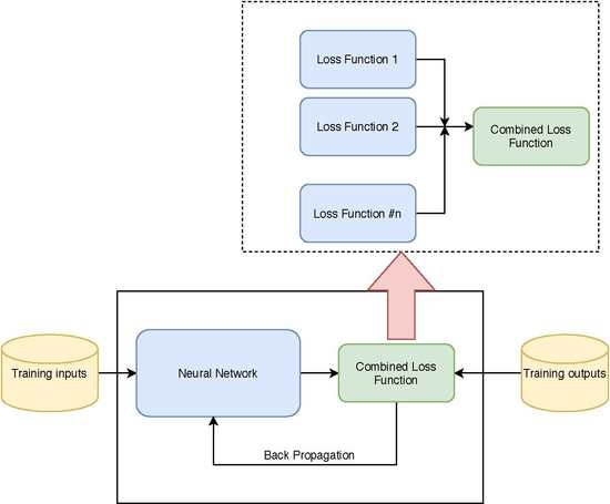
Figure 1 shows the general learning process of a neural network, which consists of two phase: training and test. The supervised learning framework generally consists of three major components which are listed as follows:
Data:
Let denote all samples where are the inputs including temperature, timespan, etc., and are the generated power in the given timespan which and .
Model:
This represents the relationship between the independent variable and the dependent variable y. For example, if there is a linear relationship between the independent variable and the dependent variable y, the model would be as follows:
Loss Function:
A loss function which measures the accuracy of the predicted label based on the true label is an important element of a learning system. The loss function is defined as a function where y is the true label and denotes the predicted label. The most intuitive loss function for regression is square loss function which is defined as follows:
The learning algorithm intends to find the regressor which is optimal in the sense that it minimizes the expected loss function defined as
where is the joint probability distribution over X and Y. Generally cannot be computed because the distribution is unknown. However, an approximation of which is called empirical risk can be computed by averaging the loss function over the training set containing N samples [21],
As it is shown in Equation (2), the loss function has an important role in the optimization problem and finding the regressor. More precisely, loss functions assign a value to each sample representing how much that sample contributes to solving the optimization problem. If an outlier is given a very large value by the loss function, it might dramatically affect the obtained learner [22]. To better explain our purpose, three loss functions with different behaviour with respect to errors are explained in the following.
The absolute loss function which linearly penalizes samples is defined as follows:
where y is the true label and is the predicted one. We denote as the distance between the predicted label and the true one. As it is shown in Figure 2, the value that Absolute loss function assigns to each sample is linearly dependent to the distance.
Square loss function is convex; hence, the advantage of optimization under the square loss function is that it leads us to a global optimum. Square loss is defined as follows:
It penalizes samples with the square of the distance. Therefore, an outlier (i.e., a very noisy sample with big ) would receive a very large number, which means that its contribution to solving the optimization problem will be significant. Therefore, it is not robust against the outliers.
Correntropy which is rooted in the Renyi’s entropy is a local similarity measure. It is based on the probability of how much two random variables are similar in the neighbourhood of the joint space. The C-loss function, which is defined in the following equation, is inspired by Correntropy criteria and is known as a robust loss function [23]. Several researchers have used the C-loss function to improve the robustness of their learning algorithms [24]. The C-loss function is defined as follow:
The three mentioned loss functions are depicted in Figure 2. There are many other different loss functions with their own characteristics making them suitable for a certain application. Inspired by ensemble methods, in this paper we propose the integration of an ensemble of loss functions into a deep neural network to forecast the generated power of a PV panel.
The ensemble technique is one of the most influential learning approaches, which theoretically boost weak learners whose accuracy is slightly better than random guesses, into arbitrarily accurate strong learners [22].
In this paper, in addition to integration of ensemble of loss functions into deep networks, we also propose a new objective function which is a combination of several loss functions. By doing so we aim to produce a strong ensemble objective function which inherits the advantages of each individual loss function. Improvement of the results when applying a linear combination of two loss functions is proved in [25,26]. Ensemble methods have also been applied to loss functions in [22].
We use three loss functions as the base losses (C-loss, absolute, square). While these three loss function have quite good performance individually, we combine them to reach a stronger regressor.
These three loss functions act differently against noise. C-loss is less sensitive to outliers since it is a bounded function. It, therefore, leads to robust classifiers. Absolute loss penalizes samples linearly, and square loss function is a very popular loss function because it leads an easy optimization reaching the global optimum; however, it significantly penalizes samples, which makes it very sensitive to noise.
4. The Proposed Method
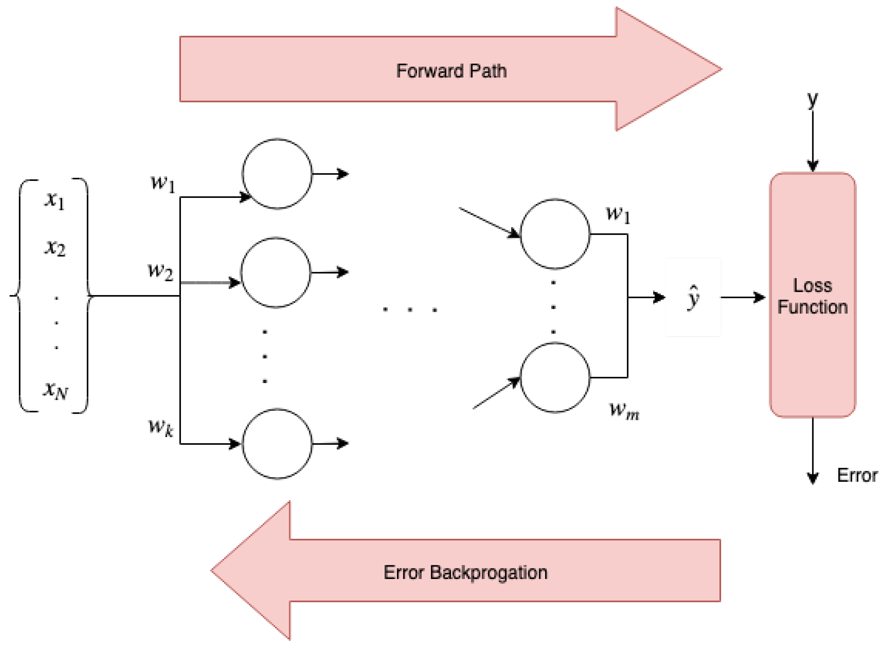
Deep Learning networks are strong methods in the field of machine learning that can solve either classification or regression problems [27]. Deep networks consist of an input layer and an output layer and several hidden layers. By employing hidden layers, whose neurons are not directly connected to the output, the network would be able to solve the non-linear problems. Figure 3 shows a neural network containing the forward path and the backward path.
Let denote the ith sample where represents the input and the true output. In the forward path, the estimated value for each sample is estimated. Let W be the weights of the network with a sigmoid function on top (to normalize data), the estimated output would be .
The aim of the neural network is to make the estimated output closer to the true label. It minimizes the average value of loss function over all samples with respect to the network’s weights. The neural network starts with initial values for weights and in the backward path, the gradient of the loss function flows back through the network and update all the weights in the opposite direction of the gradient. Therefore, the loss function has an important role in a neural network’s performance.
We propose using a Deep Learning model with one hidden layer. We make use of the ensemble loss function mentioned in Section 3. The ensemble loss function inherits the merits of each individual loss and will get better performance in the learning process. We choose three loss functions including Absolute, Square and Correntropy with different characteristics. As we mentioned in the previous section, each of these loss functions has different behaviours with respect to the noisy samples.
To avoid getting overfitted on the data, we use a regularization term which not only avoid overfilling, but also increases the network’s ability to generalization and hence, the network would work well with the unseen data as well. The whole objective function with the regularization term is defined as follow:
where denotes the three loss functions and W is the network’s weights.
To update the weights of the network and the weights associated to each loss function, we reformulate the cost function proposed in Equation (6) as follows:
The second term avoids from approaching zero values. The gradient of this new cost function then flows back through the network to update all parameters including weights of network and as well.
Three loss functions which are combined in our proposed method are Absolute, Square and Correntropy loss functions, which are depicted in Figure 2. We use the objective function (7) as the last layer of the neural network. The weights assigned to each individual loss function as well as network’s weights are updated through the backpropagation stage in which the error flow back to the network and the weights are updated accordingly.
5. Experimental Results
The presented model in the this paper has been tested and verified using the data of 39 kW photovoltaic power plant of Birjand University located in Birjand city in South Khorasan province of Iran. This data includes power output (kW), measurements of temperature and solar radiation intensity for 30 days, which are measured and recorded at intervals of 5 min during 24 h a day by the plant’s automatic metering devices. Out of the total 39 kW generation capacity of this power plant, 30 kW is connected to the grid and 9 kW is separated from the grid. We used of data for testing phase and for training. We employed 10 fold cross-validation to tune the system’s parameters.
We used a Deep Learning model with two hidden layers containing 32 and 25 nodes respectively. Each layer follows by a ReLu activation function. regularization term is used to simplify the model and avoid overfitting.
We compared our method with other regression algorithms including Ridge Regression, Bayesian Regression, kNN Regression, Decision Tree and SVR. All of the methods obtained good results while ours outperforms the other methods. We used the value 5 for kNN algorithm.
Table 1 provides mean absolute error which is calculated by for each method separately. The results show that although our approach does not get the best result for training, it performed the best on test data. Therefore, its performance is the best on unseen data.
The results also show that our method prevented overfitting. Overfitting refers to a model that fits the training data too well. Overfitting happens when a model learns the details and noise in the training data to the extent that it negatively impacts the performance of the model on new data.
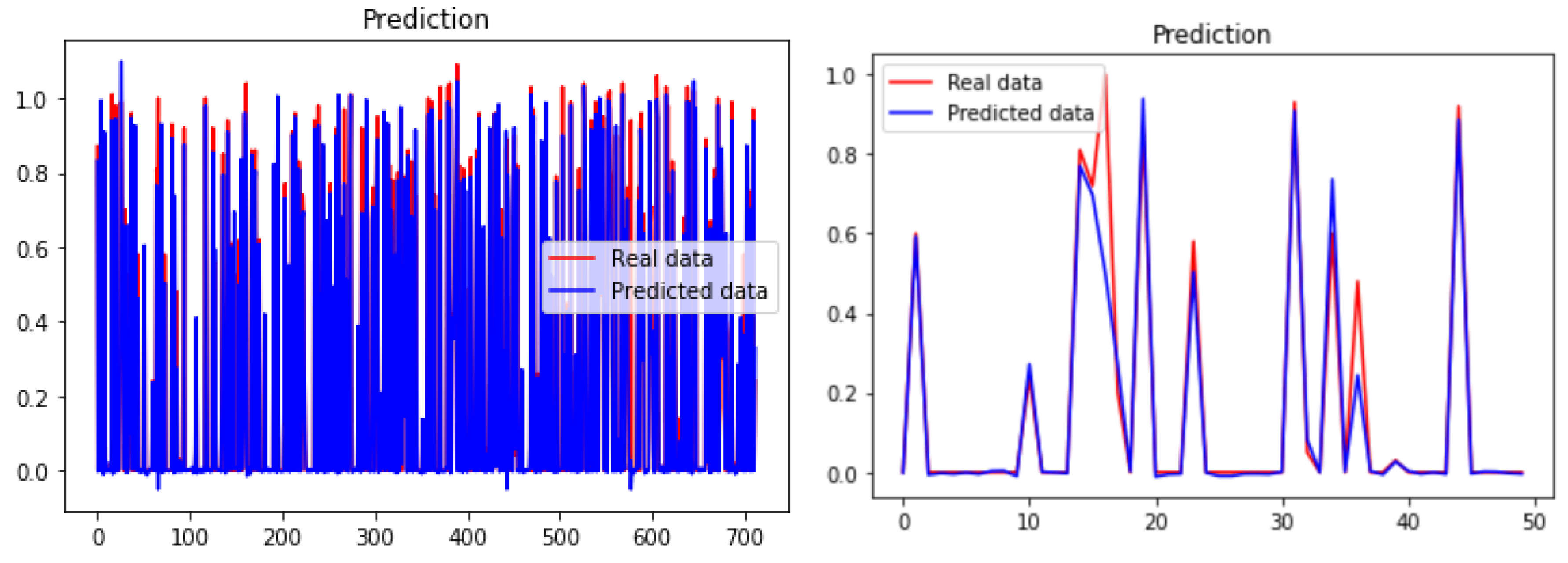
Figure 4 shows the predicted output compared with the real output. As it is shown, the predicted and true outputs are almost similar. We show a zoomed curve in the right. The blue lines are the true labels and the red one is the predicted values.
Figure 5 shows the loss value during the training and test phase. As the curves illustrate it does not overfit.
6. Conclusions
In this paper, we proposed a new objective function which is a combination of three individual loss functions. Next, a deep neural network has been extended with the proposed objective function. Performance of the proposed method is evaluated numerically based on real measurement data from a real PV power generator panel. Our performance evaluations confirm that deep neural networks trained using the combined loss function outperform the peer methods listed in Table 1 for predicting the generated power with PV panels. Moreover, according to our experiments (Figure 5), the gradient descent method converged fast.
Author Contributions
Formal analysis, M.H., M.F. and V.B.; methodology, M.H., M.F. and V.B.; software, M.H., M.F. and V.B.; supervision, M.F. and A.E.; writing—original draft, M.H., M.F., V.B. and A.E.; writing—review and editing, M.F. and A.E. All authors have read and agreed to the published version of the manuscript.
Funding
This research received no external funding.
Acknowledgments
The authors of this paper would like to thank for delivering the data of University of Birjand Solar Power Plant to the head of “Power and Energy Smart Systems Research Center”, Hamid Reza Najafi and the Department of Power Engineering of Birjand University.
Conflicts of Interest
The authors declare no conflict of interest.
References
- Liu, J.; Fang, W.; Zhang, X.; Yang, C. An improved photovoltaic power forecasting model with the assistance of aerosol index data. IEEE Trans. Sustain. Energy 2015, 6, 434–442. [Google Scholar] [CrossRef]
- Yang, D.; Kleissl, J.; Gueymard, C.A.; Pedro, H.T.; Coimbra, C.F. History and trends in solar irradiance and PV power forecasting: A preliminary assessment and review using text mining. Sol. Energy 2018, 168, 60–101. [Google Scholar] [CrossRef]
- Estebsari, A.; Pons, E.; Patti, E.; Mengistu, M.; Bompard, E.; Bahmanyar, A.; Jamali, S. An IoT realization in an interdepartmental real time simulation lab for distribution system control and management studies. In Proceedings of the 2016 IEEE 16th International Conference on Environment and Electrical Engineering (EEEIC), Florence, Italy, 7–10 June 2016; pp. 1–6. [Google Scholar]
- Estebsari, A.; Pons, E.; Huang, T.; Bompard, E. Techno-economic impacts of automatic undervoltage load shedding under emergency. Electr. Power Syst. Res. 2016, 131, 168–177. [Google Scholar] [CrossRef] [Green Version]
- Wolff, B.; Kuhnert, J.; Lorenz, E.; Kramer, O.; Heinemann, D. Comparing support vector regression for PV power forecasting to a physical modeling approach using measurement, numerical weather prediction, and cloud motion data. Sol. Energy 2016, 135, 197–208. [Google Scholar] [CrossRef]
- Zhang, W.; Quan, H.; Gandhi, O.; Rodríguez-Gallegos, C.D.; Sharma, A.; Srinivasan, D. An ensemble machine learning based approach for constructing probabilistic pv generation forecasting. In Proceedings of the 2017 IEEE PES Asia-Pacific Power and Energy Engineering Conference (APPEEC), Bangalore, India, 8–10 November 2017; IEEE: Piscataway, NJ, USA, 2017; pp. 1–6. [Google Scholar]
- Wang, K.; Qi, X.; Liu, H. A comparison of day-ahead photovoltaic power forecasting models based on deep learning neural network. Appl. Energy 2019, 251, 113315. [Google Scholar] [CrossRef]
- Estebsari, A.; Rajabi, R. Single Residential Load Forecasting Using Deep Learning and Image Encoding Techniques. Electronics 2020, 9, 68. [Google Scholar] [CrossRef] [Green Version]
- Behera, M.K.; Nayak, N. A comparative study on short-term PV power forecasting using decomposition based optimized extreme learning machine algorithm. Eng. Sci. Technol. Int. J. 2020, 23, 156–167. [Google Scholar] [CrossRef]
- Ogliari, E.; Dolara, A.; Manzolini, G.; Leva, S. Physical and hybrid methods comparison for the day ahead PV output power forecast. Renew. Energy 2017, 113, 11–21. [Google Scholar] [CrossRef]
- Wolff, B.; Lorenz, E.; Kramer, O. Statistical learning for short-term photovoltaic power predictions. In Computational Sustainability; Springer: Cham, Switzerland, 2016; pp. 31–45. [Google Scholar]
- Almeida, M.P.; Perpinan, O.; Narvarte, L. PV power forecast using a nonparametric PV model. Sol. Energy 2015, 115, 354–368. [Google Scholar] [CrossRef] [Green Version]
- Wang, F.; Zhen, Z.; Wang, B.; Mi, Z. Comparative study on KNN and SVM based weather classification models for day ahead short term solar pv power forecasting. Appl. Sci. 2018, 8, 28. [Google Scholar] [CrossRef] [Green Version]
- Dolara, A.; Grimaccia, F.; Leva, S.; Mussetta, M.; Ogliari, E. A physical hybrid artificial neural network for short term forecasting of PV plant power output. Energies 2015, 8, 1138–1153. [Google Scholar] [CrossRef] [Green Version]
- Li, Z.; Rahman, S.; Vega, R.; Dong, B. A hierarchical approach using machine learning methods in solar photovoltaic energy production forecasting. Energies 2016, 9, 55. [Google Scholar] [CrossRef] [Green Version]
- Li, Z.; Zang, C.; Zeng, P.; Yu, H.; Li, H. Day-ahead hourly photovoltaic generation forecasting using extreme learning machine. In Proceedings of the 2015 IEEE International Conference on Cyber Technology in Automation, Control, and Intelligent Systems (CYBER), Shenyang, China, 8–12 June 2015; IEEE: Piscataway, NJ, USA, 2015; pp. 779–783. [Google Scholar]
- Teo, T.T.; Logenthiran, T.; Woo, W.L. Forecasting of photovoltaic power using extreme learning machine. In Proceedings of the 2015 IEEE Innovative Smart Grid Technologies-Asia (ISGT ASIA), Bangkok, Thailand, 3–6 November 2015; IEEE: Piscataway, NJ, USA, 2015; pp. 1–6. [Google Scholar]
- Su, D.; Batzelis, E.; Pal, B. Machine Learning Algorithms in Forecasting of Photovoltaic Power Generation. In Proceedings of the 2019 International Conference on Smart Energy Systems and Technologies (SEST), Porto, Portugal, 9–11 September 2019; IEEE: Piscataway, NJ, USA, 2019; pp. 1–6. [Google Scholar]
- Reddy, S.S. Bat algorithm-based back propagation approach for short-term load forecasting considering weather factors. Electr. Eng. 2018, 100, 1297–1303. [Google Scholar] [CrossRef]
- Rego, L.; Sumaili, J.; Miranda, V.; Francês, C.; Silva, M.; Santana, A. Mean shift densification of scarce data sets in short-term electric power load forecasting for special days. Electr. Eng. 2017, 99, 881–898. [Google Scholar] [CrossRef]
- Holland, M.J.; Ikeda, K. Minimum proper loss estimators for parametric models. IEEE Trans. Signal Process. 2016, 64, 704–713. [Google Scholar] [CrossRef]
- Hajiabadi, H.; Molla-Aliod, D.; Monsefi, R. On Extending Neural Networks with Loss Ensembles for Text Classification. In Proceedings of the Australasian Language Technology Association Workshop 2017, Brisbane, Australia, 6–8 December 2017; pp. 98–102. [Google Scholar]
- Liu, W.; Pokharel, P.P.; Principe, J.C. Correntropy: A localized similarity measure. In Proceedings of the 2006 IEEE International Joint Conference on Neural Network Proceedings, Vancouver, BC, Canada, 16–21 July 2006; IEEE: Piscataway, NJ, USA, 2006; pp. 4919–4924. [Google Scholar]
- Peng, J.; Du, Q. Robust joint sparse representation based on maximum correntropy criterion for hyperspectral image classification. IEEE Trans. Geosci. Remote Sens. 2017, 55, 7152–7164. [Google Scholar] [CrossRef]
- Shi, Q.; Reid, M.; Caetano, T.; Van Den Hengel, A.; Wang, Z. A Hybrid Loss for Multiclass and Structured Prediction. IEEE Trans. Pattern Anal. Mach. Intell. 2015, 37, 2–12. [Google Scholar] [CrossRef] [PubMed]
- BenTaieb, A.; Kawahara, J.; Hamarneh, G. Multi-Loss Convolutional Networks for Gland Analysis in Microscopy. In Proceedings of the Biomedical Imaging (ISBI 2016), Prague, Czech Republic, 13–16 April 2016; pp. 642–645. [Google Scholar]
- Rajabi, R.; Estebsari, A. Deep Learning Based Forecasting of Individual Residential Loads Using Recurrence Plots. In Proceedings of the 2019 IEEE Milan PowerTech, Milan, Italy, 23–27 June 2019; pp. 1–5. [Google Scholar]
Figure 1.
The supervised learning framework.

Figure 2.
The Absolute loss (red), the Square loss (blue) and the Correntropy loss function (green).
Figure 2.
The Absolute loss (red), the Square loss (blue) and the Correntropy loss function (green).

Figure 3.
A deep learning network.

Figure 4.
(Left) The predicted labels compared with the true labels. (Right) Zoomed curve of the predicted and real labels.
Figure 4.
(Left) The predicted labels compared with the true labels. (Right) Zoomed curve of the predicted and real labels.

Figure 5.
Loss values during train and testing phases.


Table 1.
Mean absolute error (MAE) for testing and training phase.
| Method | Training Error | Test Error |
|---|---|---|
| Ridge Regression | 0.000488 | 0.005673 |
| kNN Regression | 0.000242 | 0.003482 |
| Bayesian Regression | 0.000488 | 0.005672 |
| Decision Tree | 0.001040 | 0.012720 |
| SVR | 0.000842 | 0.009866 |
| The Proposed Method | 0.000335 | 0.002785 |
© 2020 by the authors. Licensee MDPI, Basel, Switzerland. This article is an open access article distributed under the terms and conditions of the Creative Commons Attribution (CC BY) license (http://creativecommons.org/licenses/by/4.0/).
Share and Cite
MDPI and ACS Style
Hajiabadi, M.; Farhadi, M.; Babaiyan, V.; Estebsari, A. Deep Learning with Loss Ensembles for Solar Power Prediction in Smart Cities. Smart Cities 2020, 3, 842-852. https://doi.org/10.3390/smartcities3030043
AMA Style
Hajiabadi M, Farhadi M, Babaiyan V, Estebsari A. Deep Learning with Loss Ensembles for Solar Power Prediction in Smart Cities. Smart Cities. 2020; 3(3):842-852. https://doi.org/10.3390/smartcities3030043
Chicago/Turabian StyleHajiabadi, Moein, Mahdi Farhadi, Vahide Babaiyan, and Abouzar Estebsari. 2020. "Deep Learning with Loss Ensembles for Solar Power Prediction in Smart Cities" Smart Cities 3, no. 3: 842-852. https://doi.org/10.3390/smartcities3030043