Article

Synergetic Use of Sentinel-1 and Sentinel-2 Data for Wheat-Crop Height Monitoring Using Machine Learning

by
Lwandile Nduku
1,2,*,
Cilence Munghemezulu
2,
Zinhle Mashaba-Munghemezulu
2,
Phathutshedzo Eugene Ratshiedana
2,
Sipho Sibanda
2 and
Johannes George Chirima
1,2
1
Department of Geography, Geoinformatics & Meteorology, University of Pretoria, Pretoria 0028, South Africa
2
Agricultural Research Council—Natural Resources and Engineering, Private Bag X79, Pretoria 0001, South Africa
*
Author to whom correspondence should be addressed.
AgriEngineering 2024, 6(2), 1093-1116; https://doi.org/10.3390/agriengineering6020063
Submission received: 3 March 2024 / Revised: 15 April 2024 / Accepted: 16 April 2024 / Published: 22 April 2024
(This article belongs to the Special Issue Application of Remote Sensing and GIS in Agricultural Engineering)

Abstract

:
Monitoring crop height during different growth stages provides farmers with valuable information important for managing and improving expected yields. The use of synthetic aperture radar Sentinel-1 (S-1) and Optical Sentinel-2 (S-2) satellites provides useful datasets that can assist in monitoring crop development. However, studies exploring synergetic use of SAR S-1 and optical S-2 satellite data for monitoring crop biophysical parameters are limited. We utilized a time-series of monthly S-1 satellite data independently and then used S-1 and S-2 satellite data synergistically to model wheat-crop height in this study. The polarization backscatter bands, S-1 polarization indices, and S-2 spectral indices were computed from the datasets. Optimized Random Forest Regression (RFR), Support Vector Machine Regression (SVMR), Decision Tree Regression (DTR), and Neural Network Regression (NNR) machine-learning algorithms were applied. The findings show that RFR (R2 = 0.56, RMSE = 21.01 cm) and SVM (R2 = 0.58, RMSE = 20.41 cm) produce a low modeling accuracy for crop height estimation with S-1 SAR data. The S-1 and S-2 satellite data fusion experiment had an improvement in accuracy with the RFR (R2 = 0.93 and RMSE = 8.53 cm) model outperforming the SVM (R2 = 0.91 and RMSE = 9.20 cm) and other models. Normalized polarization (Pol) and the radar vegetation index (RVI_S1) were important predictor variables for crop height retrieval compared to other variables with S-1 and S-2 data fusion as input features. The SAR ratio index (SAR RI 2) had a strong positive and significant correlation (r = 0.94; p < 0.05) with crop height amongst the predictor variables. The spatial distribution maps generated in this study show the viability of data fusion to produce accurate crop height variability maps with machine-learning algorithms. These results demonstrate that both RFR and SVM can be used to quantify crop height during the growing stages. Furthermore, findings show that data fusion improves model performance significantly. The framework from this study can be used as a tool to retrieve other wheat biophysical variables and support decision making for different crops.

1. Introduction

In recent years, the Food and Agriculture Organization (FAO) reports show an increasing demand for wheat production to meet the world’s current population’s consumption [1,2,3]. Wheat is the world’s largest cultivated cereal crop, covering approximately 220.62 ha (million hectares) in 2022/23 [1,4]. Wheat products contribute significantly to eradicating hunger, reducing poverty, and achieving global food security, which are central to the United Nations Sustainable Development Goals (SDGs) number 1 and number 2 [5,6,7,8]. The SDG 1 pertains to the eradication of poverty in all its manifestations worldwide, whereas SDG 2 focuses on ending hunger, attaining food security, enhancing nutrition, and fostering sustainable agriculture. However, several factors have gradually reduced wheat production over the years contributing to the increasing demands estimated at 70% for a population of 10 billion by 2050 [9,10,11,12]. The declining trend in wheat production is due to socio-economic factors, as well as abiotic and biotic stresses that have negative impacts on crop growth conditions and food security [13,14,15,16]. Abiotic stress factors include extreme heat, drought, frost, salinity, waterlogging, and nutrient deficits, while biotic stresses are due to crop diseases, weeds, and pests [17,18,19]. Crop height is one of the important agronomic indicators related to production, providing an indication of crop stress and essential information and alerts about intra-field crop health conditions. Therefore, monitoring crop height throughout the growing season is critical to understanding the anticipated yields as well as improving wheat production forecasting.
The traditional methods such as Light Detection and Ranging (LiDAR) and Unmanned Aerial Services (UAS) have high accuracy when monitoring crop height development [20,21,22,23,24]. Another accurate manual approach for crop height measurement is using a yardstick (ruler or meter scale) [20,21]. However, these approaches are generally time-consuming, expensive, labor-intensive, prone to human error, and unable to generate digital crop-height spatial distribution maps for large-scale farms [22,25,26,27]. Remote sensing satellite data have shown great potential to alleviate limitations of traditional measurements due to the satellites’ efficiency, digital wide intra-field of view, and ability to revisit time characteristics, which are key for accurate monitoring of crop biophysical parameters [28,29,30,31,32]. The S-1 and S-2 satellite sensors offer high-resolution imagery and revisit time data for monitoring agricultural applications and land use/land cover changes for free [33]. The S-1 and S-2 satellite sensors have better spatial resolution compared to the moderate-resolution imaging spectroradiometer (MODIS) and Landsat collections; as a result, these sensors are useful for farm-scale applications [34,35,36]. The improvement in the spatial and spectral resolutions of both S-1 and S-2 sensors makes these satellites suitable for monitoring crop biophysical parameters such as height, among others. Additionally, both the S-1 and S-2 satellite sensors increase the frequency of data acquisition for field-scale crop monitoring. For example, the Copernicus Open Access Hub provides S-1 and S-2 images at 5-day intervals, which is suitable for timely crop monitoring and subsequent management and intervention [16]. The S-2 satellite data are affected by cloudy atmospheric conditions and rain, which limit the acquisition of data during the crop growing season [37]. However, S-2 images provide a red-edge band that is very sensitive to crops changes as the plants grow, which can help time-series monitoring. The S-1 satellite can provide data that are not obstructed by clouds and can complement S-2 satellite images [38,39]. Previous studies showed that there is a strong relationship between crop height and S-1 satellite variables with 66%, 82%, and 92% precision for wheat-height estimation, respectively [40,41,42]. These S-1 satellite imagery variables include local incidence angle normalization, Alpha (α) and dual-polarization VV (vertical transmits and vertical receive), and VH (vertical transmit and horizontal receive). Furthermore, the application of S-1 satellite data has revealed 66% and 68% sensitivity for wheat-crop height estimation with linear regression (LR) and exponential models, respectively [43,44]. The Alpha (α) decomposition parameter has achieved a 67% wheat-crop height sensitivity prediction based on the use of SAR data [42]. The use of S-1 satellite data has produced 87% and 62% correlations with RFR and LR for wheat-crop height sensitivity estimation [45]. Nevertheless, S-1 satellite data have not been investigated extensively for agricultural applications because of the complex data structure, in comparison to S-2 satellite data [35,46,47].
The synergistic use of SAR S-1 and optical S-2 sensors provides feasibility of capturing both spectral and textural information [35,40,48,49]. Additionally, the fusion of both S-1 and S-2 satellite data has been reported to improve the estimation accuracy of different biophysical parameters with the application of machine-learning algorithms [48,49,50]. For example, RFR and particle filter (PF) models have achieved 92% and 95% correlation coefficient precision for estimation of rice-plant height using S-1 satellite data, respectively [41,51]. Furthermore, the LR model obtained 66% accuracy with SAR data for estimating wheat-crop height. Kaplan et al. [40] have found that the Enhanced Vegetation Index (EVI) and the local incidence angle normalization model attained 88% and 66% precision for estimating cotton crop height using SAR and optical data, respectively. The local incidence angle normalization method has achieved accuracies of 86% and 87% for wheat and cotton-crop height estimation using SAR imagery [52]. The crop coefficient (Kc) model achieved more than 80% estimation accuracy for tomato-crop heights when applied to the synergetic use of S-2 MSI and VENµS imagery [53]. Abdikan et al. [49] and Xi et al. [54] also observed that the artificial neural network (ANN) model attained 91% of sunflower-crop height estimation, and the gradient boosting decision tree (GBDT) model attained 72% of forest-canopy height estimation using a S-1 and S-2 satellite data combination. In most studies, SAR and optical data are explored separately for crop height and biophysical variable estimation [40,41,49,52,55]. Recently, studies have shown that these data products display limitations when used independently, which are overcome by using them synergistically [56,57,58]. Xi et al. [54] used ICESat-2, S-1, and S-2 satellite imagery to develop a crop-height model of different forest types in China. The derived matrices from S-1 and S-2 data showed that they played a critical role in modeling different forest types. Narin et al. [45] use S-1 data to estimate the crop height of wheat in Turkey, and they found that VH was more sensitive compared to VV polarization. Ndikumana et al. [41] used multitemporal S-1 data to model rice-plant height and dry aboveground biomass in southern France. They also reported that VH was more correlated with in situ measurements compared to VV and that the RFR model yielded an accuracy of more than 80% for both height and biomass models. Similar results were obtained by Sharifi et al. [59]. Abdikan et al. [49] used both S-1 and S-2 satellite data to predict crop height of sunflower crops in Turkey. The authors found that ANN and GBDT models produced higher accuracies of more than 90% and that NDVI with a red-edge band was one of the most important contributions. However, studies that have explored the feasibility of combining S-1 and S-2 satellite data to monitor intra-season and intra-field crop height variability for winter wheat fields are limited.
This current study examines the sensitivity of VV, VH, VH–VV ratio, and S-1 polarization indices’ data to monitor the time-series monthly intra-field crop-height growth of a wheat farm. Secondly, the combined use of SAR S-1 and optical S-2 spectral indices’ time-series monthly data for monitoring intra-field crop height variability is investigated. The RFR, SVMR, DTR, and NNR machine-learning algorithms (MLAs) are applied to both experiments. Both RFR and SVMR have been shown to be effective models for estimating crop parameters in previous studies [41,60]. The selection criteria for RFR, SVMR, DTR, and NNR MLA are associated with their reported capabilities to handle nonlinear and noisy data with precision when monitoring crop biophysical variables [2,41,47,54,60]. This present study investigates the following detailed objectives: (1) assessing the relationship between intra-field crop height growth variation with S-1 VH, VV, VH–VV ratio polarizations, and S-2 vegetation indices; (2) investigating the effectiveness of the selected RFR, SVMR, DTR, and NNR algorithms in predicting crop height variations; (3) determining which input features are important for modeling crop height growth; (4) evaluating the measurement method that is fundamental for estimating crop height variation; and finally, (5) mapping the pattern of intra-field and intra-season crop height spatial distribution at the wheat-farm level.

2. Materials and Methods

2.1. Location of the Study Site

The wheat farm in Clarens is found within South Africa in the north-east part of the Free State province under the Thabo Mofutsanyane district (Figure 1). The Clarens wheat farm area receives approximately 688 mm yearly mean rainfall and has 7.8 °C and 20.7 °C minimum and maximum mean temperatures for both winter and summer periods [61]. Rainfall occurs in the summer season with hot days above 20.7 °C as the average temperature [61,62,63,64]. Sandy loam, Avalon, and Pinedene are dominant soil types in the Thabo Mofutsanyane district. These soil characteristics are moderately permeable [65]. Additionally, the district has rainfed winter wheat production within dryland areas [66,67,68]. The Thabo Mofutsanyane district experiences various climatic-related events including winter frost occurrence in most low-lying areas, as well as prolonged periods of dry spells and droughts [69,70,71,72]. These climatic events frequently affect agricultural crop production and result in reduced yields. The high-risk dependence of crop production such as wheat on rainwater within the Thabo Mofutsanyane district and surrounding areas make crops vulnerable to inconsistent changing precipitation patterns, decreasing precipitation quantity, which affects crop growth conditions [70,71,72]. The dryland wheat farm considered in this study is approximately 30 ha in size. Table 1 details the wheat-crop growth stages. The stages are divided into five-month periods, corresponding to the S-1 and S-2 overpasses. The early germination stage is characterized by radicle, coleoptile, and early leaf development. The early development stage involves tillering, head differentiation, stem growth, and head growth. The late and mature stages involve head emergence, flowering, kernel growth, and maturity. The last stage of senescence is characterized by wheat losing its greenness and leaves starting to fall off the stem. The heights were measured using measuring tape and were geolocated using a Global Positioning System (GPS) device by following the systematic sampling method.
Figure 2 shows the field and crop conditions throughout different wheat phenological stages. The following observations of the wheat (A–H) were taken during the field visit at the research farm. Subfigure (A) represents the germination stage, (B) shows the early tillering stage, (C–E) show the development stages, (F) corresponds to the grain-filling stage, and (G,H) signify the maturity stage.

2.2. Image Data Collection, Preprocessing, and Analysis

The SAR S-1 GRD collection that was downloaded in the Interferometric Wide (IW) mode covering the wheat growing period (August to November 2021) was utilized in this study. The S-1 SAR toolbox within the Sentinel Application Platform (SNAP) environment was utilized for preprocessing of S-1 imagery [73,74]. The preprocessing includes radiometric calibration, terrain correction, and removal of the border and thermal noise [75]. Applying the orbit file updates the metadata. Thermal noise removal masks artificially low backscatter pixels within the margin of an image swath [76]. Radiometric calibration is performed to generate the unitless backscatter intensity [77]. Terrain correction geo-codes the images using a digital elevation model (DEM) from the Shuttle Radar Topography Mission (SRTM) at 30 m spatial resolution [78,79,80]. Additional speckle filtering was performed on the S-1 SAR GRD data using the Lee filter to decrease the coarse noise triggered by many scatters [81]. The VV and VH S-1 polarization backscatter bands at 10 m spatial resolution were utilized to calculate the S-1 polarization indices summarized in Table 2 below.
The S-2 satellite mission consists of two polar orbiting satellites—S-2A launched in June 2015 and S-2B commissioned in July 2017. The temporal resolution and combined constellation of the S-2 MSI sensor are 10 days and 5 revisiting days, respectively. The S-2 Multispectral Instrument (MSI) sensor onboard S-2A and S-2B comprises thirteen spectral bands. These spectral bands are characterized into four bands including blue (band 2), green (band 3), red (band 4), and NIR (band 8) at 10 m resolution. Secondly, it includes six bands incorporating red edge 1 (B5), red edge 2 (B6), red edge 3 (B7), red edge 4 (band 8A), SWIR (band 11), and SWIR (band 12) at 20 m resolution. Finally, there are three bands involving coastal aerosol (band 1), water vapor (band 9), and cirrus (band 10) at 60 m resolution. The S-2 optical data are available as a level 2A product from the Copernicus Open Access Hub, where the per-pixel radiometric measurements are provided in surface reflectance [35,84,85]. The atmospherically corrected images were acquired using the Google Earth Engine (GEE) open access platform (https://earthengine.google.com/ accessed on: 19 March 2023). In this open-source platform, the L1C raw data are corrected using the Sen2Cor algorithm [86]. A threshold of cloud coverage of not more than 20% was applied, and a cloud musk layer generated by the Scene Classification Layer (SCL) algorithm within the Sen2Cor was also applied. This algorithm allows to detect clouds, their shadows and snow. The bands from S-2 MSI data were utilized to derive the following spectral indices shown in Table 3.
Figure 3 summarizes the research methods used in the current study. The bands from SAR S-1 and optical S-2 imagery were utilized to calculate vegetation indices, respectively. Furthermore, the sampled points were overlaid with a spectral vegetation index to generate spectral index values in the ArcMap GIS environment. The spectral index value datasets were split into a training set of 70% and 30% testing data. The in situ crop height measurement was used as the response variable to predict the crop growth rate using SAR S-1 images separately and a SAR S-1 and optical S-2 data fusion.

2.3. Random Forest Regression

RFR is a robust ensemble learning algorithm and non-parametric method that is commonly applied to classification and regression problems using large number of decision trees [90]. RFR uses a bootstrapping technique from input data to forecast a continuous outcome variable based on both classification and regression decision trees. All individual decision tree models are applied rigorously to fit in the data with a root node, which aggregates similar data values into subsets. Additionally, random subsets of parameters contain each node for every tree data split. Randomization of the RFR model ensures its robustness to outliers and overfitting [90]. The prediction results are based on aggregated averages of all individual trees. The selected parameters and number of trees used at each node split control the RFR model outcomes [91]. Also, optimizing the number of trees and number of parameters helps to improve model performance during the estimation process. The interactive MATLAB application products enable optimization of RFR [92]. The RFR model is applied in this study based on its superior capacity to distribute high-dimensional data and handle nonlinear noisy data at minimal overestimation [93]. RFR has found applications in various domains, including agricultural crops and image recognition, among others [94,95].

2.4. Support Vector Machine Regression

SVMR consists of supervised learning and non-parametric approaches for solving classification and regression problems [89,96,97]. The SVMR algorithm utilizes a set of kernel functions to convert datasets into usable formats [98]. Selection of kernel functions such as polynomial, sigmoid, linear, radial basis, and nonlinear varies depending on user specification when finding the optimal quadratic solution [99]. The kernels’ efficiency varies, and nonlinear kernels frequently have better outcomes [49,100,101]. Optimal performance of the SVMR model requires carefully chosen, tuned hyperparameters. Several studies have explored the common efficiency of SVMR for different crop biophysical parameters [97,102]. The present study executed the SVMR algorithm using interactive MATLAB application products.

2.5. Neural Network Regression

NNR is a learning algorithm technique that can use nonlinear data and is suitable for modeling prediction. The multilayer feed-forward network procedure is used by NNR to learn and train networks. NNR can learn complex relationships between multiple input and output features through constant adjustments of connection neuron weights and thresholds, based on backpropagated error difference of measurements and the predicted outcomes [103,104]. The minimization of errors during iterations of NNR model training is referred to as supervised learning. The optimizable NNR model for this study was run using a MATLAB application product. The NNR model properties included multilayer feed-forward architecture composed of three connected layers: first layer, second layer, and third layer with values of 4.44 and 2930, respectively. Furthermore, NNR employs the mean squared error loss function.

2.6. Decision Tree Regression

DTR is a supervised algorithm that predicts regression and classification problems using decision trees [105,106]. This non-parametric algorithm uses the tree node principle, which creates binary decisions to isolate different categories into internal nodes and numerous leaves contained in all datasets. DTR uses an interconnected parameter structure, which breaks down large and complex datasets efficiently into simpler and exclusive decisions. Decision tree regression frequently identifies the optimal algorithm and hyperparameters to subdivide input datasets for better prediction outcomes. MATLAB enables unsupervised selection of hyperparameters to identify the best model. The DTR model was constructed using a MATLAB product for this study.

2.7. Experimental Setup

The first experimental setup utilized time-series values of S-1 polarizations and polarization vegetation index data. The second experiment explored the time-series values of synergy of S-1 and S-2 spectral indices’ datasets. In both experiments, the RFR, SVMR, NNR, and DTR optimized regression models were applied. A total of 500 samples (100 samples collected monthly during different growth stages) were used in this study. These sample points were randomly selected and split into 350-sample training set (70%) and 150-sample test set (30%) for all models. Cross validation was performed using a k-fold strategy, where the number of folds for kk value is ten (k = 10) to evaluate the model accuracy. During the model training iteration, the best point and minimum error hyperparameters were used to evaluate the best performing optimized models. The optimized SVMR model in experiment 1 had the following parameters: a box constraint value of 0.1959, epsilon value of 8.7468, and a quadratic kernel function. The optimized RFR model in experiment 2 had 6 trees. The implementation of the models was performed on MATLAB software (version R2023b) [92]. The ranking of variable importance for each input feature was derived using the fitensemble function on MATLAB following the predictor importance procedure [107]. Table 4 below summaries the data configurations for the experiments. Experiment 1 used eleven S-1 variables, while experiment 2 used 20 variables of combined SAR S-1 and optical S-2 datasets. Experiment 1 and experiment 2 variables were selected because of their sensitivity to variation in crop height growth.

2.8. Assessment of Model Performance

The model performance for RFR, SVMR, DTR, and NNR was assessed using the 10-cross validation (k = 10) method. The efficiency of the above models was evaluated by comparing the retrieved wheat height with in situ crop measurements by using standard statistical metrics to measure the performance of the models, i.e., mean absolute error (MAE), root mean square error (RMSE), and correlation coefficient ( R 2 ) according to Equations (1)–(3) below.
M A E = 1 n i = 1 n y i y ^ i .
R M S E = 1 n i = 1 n Y i X i 2 ,
R 2 = i = 1 n Y i Y ¯ i X i X ¯ i i = i n Y i Y ¯ i 2 × i = i n X i X ¯ i 2 .
where n represents the number of observations, and Y i and Y ¯ i are the predicted features and their averages (means). X i and X ¯ i represent the ground truth measurement variables and their means. The correlation measures the fraction of the total sum of squares explained by the regression. RMSE measures the standard deviation of the residuals. A well-performing model would have a low RMSE and a higher R 2 [41].

3. Results

3.1. Crop Height Descriptive Summary Statistics

The number of samples (N), mean (M), standard deviation (SD), minimum (Min) and maximum (Max) descriptive statistics of wheat height as measured in the field during different growth stages (early germination, early development, late development, maturity, and senescence) are listed in Table 5. The lowest measured average height was 14.04 cm, and the maximum average height was 89.40 cm for the early germination and senescence stages, respectively. The maturity stage had the highest value of 103.5 cm, while the early germination stage had the minimum value of 4.10 cm. The mean height of the wheat increased as the crop phenological stages progressed (Figure 4). During the last two stages of maturity and senescence, the crop height was constant.

3.2. Correlation Matrix and Statistical Summary from S-1 and S-2 Satellite Data

Figure 5 depicts the correlation matrix between the measured height and derived features from SAR S-1 and optical S-2 imagery. Only SARRI2 had a strong positive correlation and was significant at a 95% level (r = 0.94; p < 0.05) for crop height. Additionally, the crop height had a positive correlation with VV, SAR RI 1, VH, and VH + VV, respectively. NDRE1, NDRE2, NDVI, SAVI, DVI, EVI, and CIRE were strongly positive and significantly correlated with each other. This implies a strong sensitivity of the above vegetation indices to crop growth; the height increases with leaf development as the season progresses. The negative and insignificant correlation observed between S-1 SAR and S-2 MSI features cannot be generalized but is attributed to the features’ capacity to detect crop height changes as the wheat crop develops.
Table A1 lists the statistics of the derived mean from S-1 polarization backscatter bands, polarization backscatter, and S-2 spectral indices over time. As expected, for S-2 MSI vegetation indices such as NDVI, NDVRE 1, NDVRE 2, RVI_S 2, and CIRE, the mean values increase as the growth stages advance but decrease during the senescence stage. The coefficient of variation (CV) remained relatively low at an average of 25% during the first four months. However, during the senescence stage, the CV increased to 64%. This suggests that the greenness of wheat within the farm had very few variations during the first four months, while the senescence stage was characterized by browning of the leaves resulting in a high CV value. The mean values of backscatter polarization bands and polarization indices varied in intensity during the crop growth stages. The standard deviations also indicate similar variations.

3.3. Derived Crop Height Model Accuraccy

The SVMR and RFR model performance statistics for intra-field crop height calculated using S-1 data (experiment 1) and the S-1 + S-2 data fusion (experiment 2) are summarized in Table 6 and Table 7. SVM yielded higher accuracies (R2 = 0.58, RMSE = 20.41 cm) in comparison to RFR (R2 = 0.56, RMSE = 25.34 cm), DTR (R2 = 0.52, RMSE = 21.95 cm), and NNR (R2 = 0.57, RMSE = 20.71 cm) for crop height estimation with a training set of S-1 data (experiment 1). Inversely, the S-1 + S-2 (experiment 2) data fusion generated more precise crop height estimation with RFR (R2 = 0.93 and RMSE = 8.53 cm) in comparison to SVMR (R2 = 0.91 and RMSE = 9.20 cm), NNR (R2 = 0.84, RMSE = 12.48 cm), and DTR (R2 = 0.80, RMSE = 14.02 cm) during the training sets of models. Experiment 1 test set data had higher accuracies with minimal difference compared to the training set, which indicates that there was no overfitting in all models. Additionally, the low average of 3.5 precision between training-set and test-set accuracy in experiment 2 shows that enough data were generated for all models to minimize overfitting.
The scatterplots were constructed based on the best performing training set of RFR and SVMR models in both experiments to show the multicollinearity between predicted and observed wheat-crop height (Figure 6 and Figure 7). The clustered points along the regression lines show a relationship between the predicted and observed wheat-crop height values for RFR and SVMR machine learning regression models using S-1 SAR data separately and the S-1 with S-2 satellite data fusion. RFR (R2 = 0.93 and RMSE = 8.43 cm) slightly outperformed SVMR (R2 = 0.91 and RMSE = 9.20 cm) and other models at a 95% confidence interval utilizing the S-1 SAR and S-2 MSI data fusion. However, there was contrariwise performance of SVM (R2 = 0.58 and RMSE = 20.41 cm) performing better than the RFR (R2 = 0.56 and RMSE = 21.01 cm) model with S-1 SAR data.

3.4. Ranking of Feature Importance

The variable importance of each feature was investigated for the best performing RFR and SVMR machine learning models in both experiments (Figure 8 and Figure 9). Variable predictor importance varied for both trained models. The training set of the RFR model using S-1 data showed that the most important predictors were VV × VH and SAR RI 1, while during the training set of the RFR model using the SAR S-1 and optical S-2 data fusion, the most important predictors were RVI_S1 and Pol among others. However, the SVMR model ranked VV × VH, SAR RI 1, and VV highly based on the S-1 satellite data training set, whereas the highest rankings were RVI_S1, Pol, and SAR SDI from the combined data from SAR S-1 and optical S-2 data training of the SVMR model. In general, RVI_S1 and Pol were the most important input predictors for both the RFR and SVMR models during data fusion and yielded higher model accuracies. The variable importance of S-2 data was zero in all the experiments. This means that wheat-crop height can be accurately predicted utilizing only S-1 SAR data and its indices. For example, Nasirzadehdizaji et al. [42] carried out sensitive analysis of multitemporal S-1 parameters to crop height and canopy coverage. The authors found that VV and VH produced a coefficient determination of about 80% for maize, sunflower, and wheat. Khabbazan et al. [108], Vavlas et al., [109] and Yang et al. [51] showed that S-1 satellite data can be used successfully for crop height monitoring. In contrast, Mercier et al. [110] and Abdikan et al. [49] reported that S-2 MSI data were one of the most important types of data in accurately mapping crop height. Data integration for crop height modeling should be further investigated.

3.5. Estimated and Measured Intra-Season Wheat-Height Variability

The in situ measurement and estimation of intra-season wheat-height growth were compared to the RFR and SVMR machine learning models (Figure 10). An increasing trend in crop height estimation is expected as the crop growth stages progress. The measured wheat height and RFR estimation were similar at the early development stages, while SVMR overestimated the crop height. During the late crop development stages, both RFR and SVM overestimated crop height in comparison to measured height. However, both RFR and SVMR underestimated the crop height growth at the maturity and senescence stages. These findings can be attributed to the limitations in the models’ ability to capture the complex dynamics of crop growth during later stages and insufficient training data representing the full range of growth patterns and biases in the input data used for training the models. Also, the sensitivity of the crop height decreases with increasing vegetation cover growth [42]. The study suggests that the RFR model offers an alternative method for crop height estimation in large-scale agricultural fields for crop management practices, avoiding time-consuming in situ measurement.

3.6. Mapping Intra-Season Crop Height Variability for the Wheat Farm

The intra-field and intra-season crop height variability is mapped in Figure 11. The RFR (a–e) and SVMR (f–j) models in Figure 11 show differences in the spatial distribution maps of wheat-crop height between August and November, respectively. During the first two months of August and September, which represent the early months of the season, there were variations in the performances of RFR (a), (b) and SVMR (f), (g). They both depict poor spatial variability of the crop height. During the last two months of the season, October and November, both models, as shown in Figure 11c–e and Figure 11h–j, produced similar results with higher accuracies in the estimation of crop height, respectively. Overall, SVMR, as seen in Figure 11j, had equal and higher distributions of crop height prediction compared to the lower crop height estimation in central Figure 11e, which shows results from the RFR wheat farm. These monthly spatial distribution maps provide a digital field overview of wheat growth changes, which is useful for timely crop management practices. Therefore, accurate maps may result in improvement of decision making during intra-field visits for the nutrient fertilizer use efficiency required to increase crop productivity.

4. Discussion

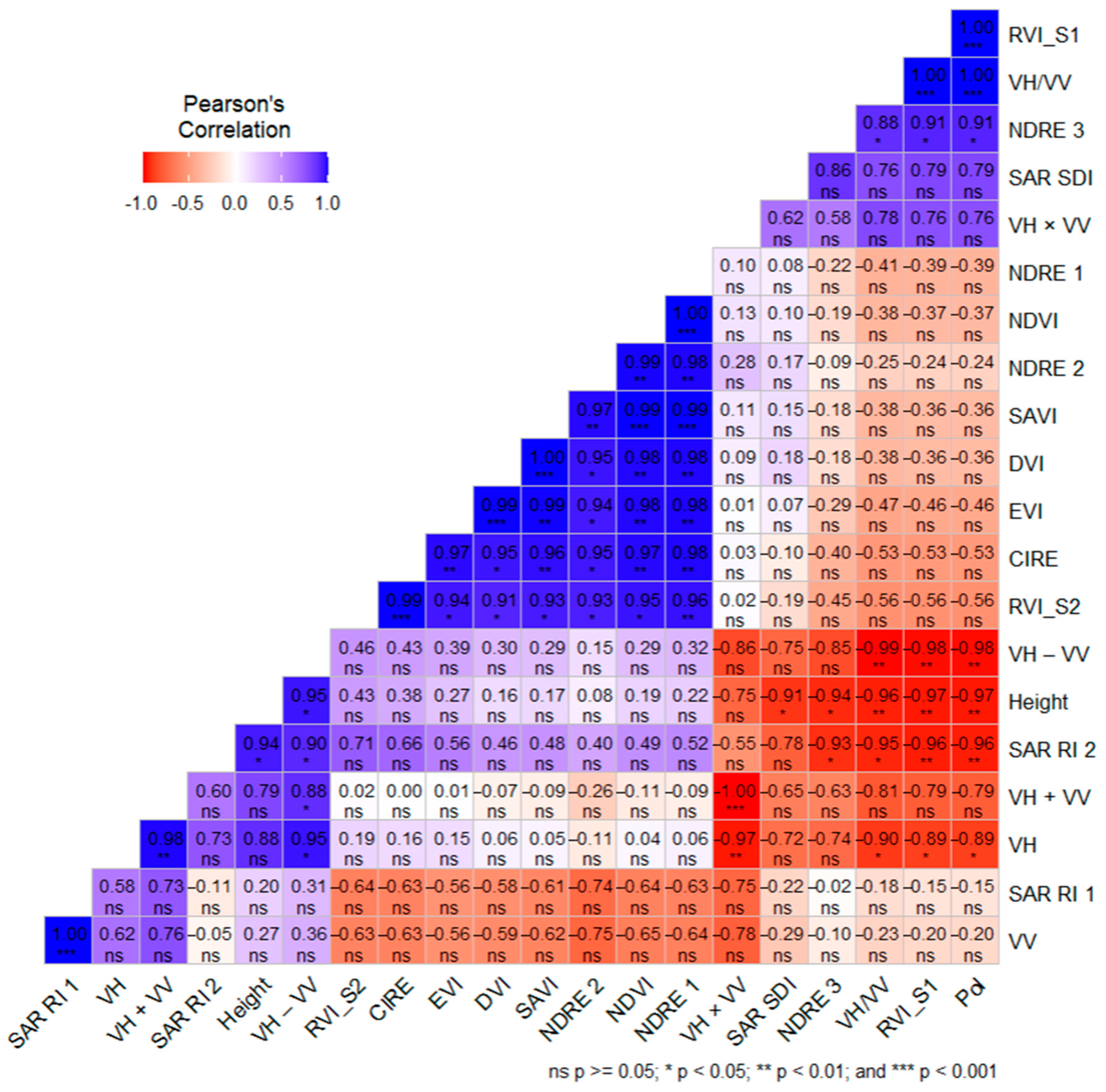
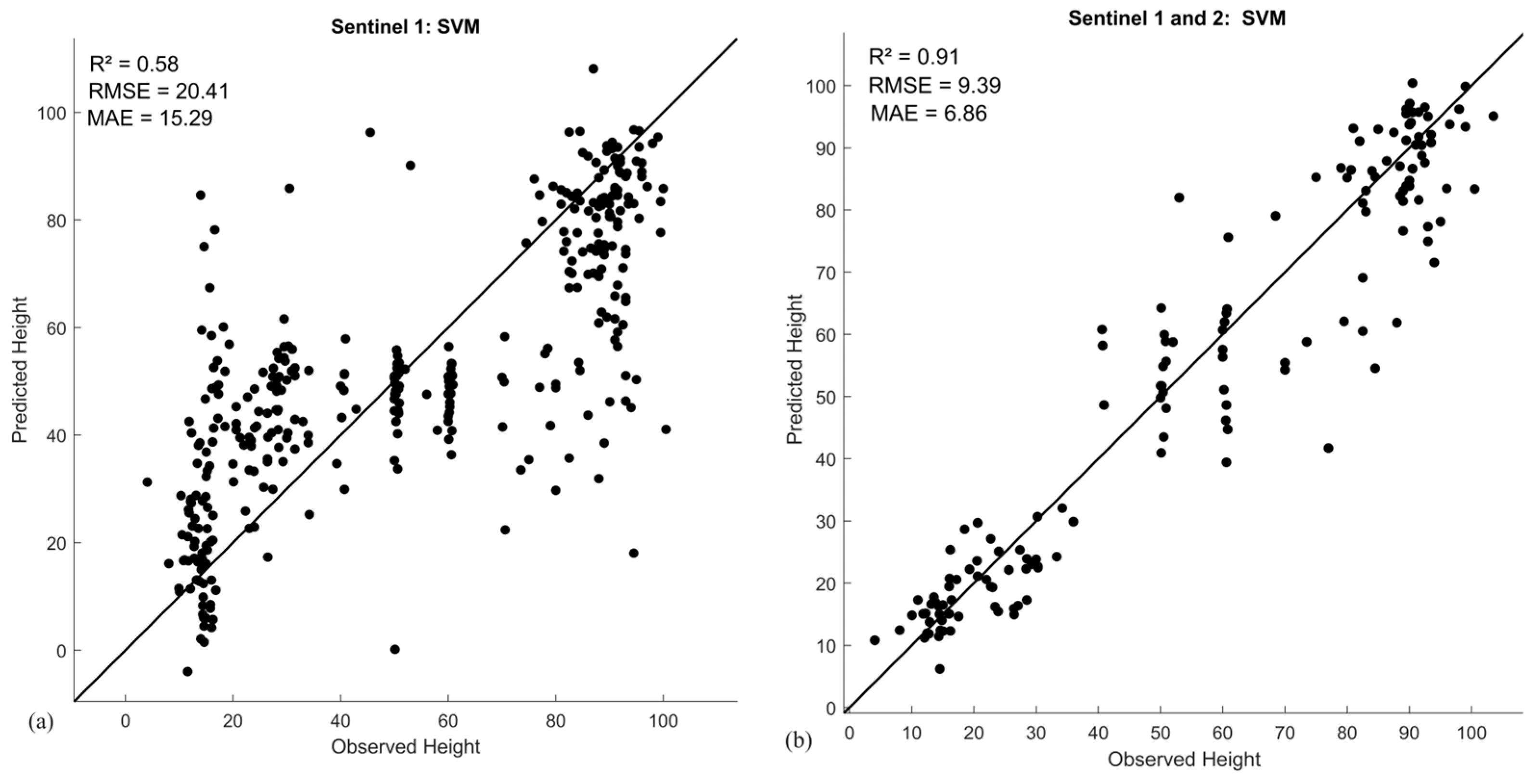
This study evaluated the feasibility of S-1 polarization backscatter bands, S-1 polarization indices, and data integration of S-1 and S-2 spectral indices for predicting intra-field and intra-season crop height variation in the wheat farm of Free State Clarens. Crop height was investigated for the different development stages. RFR, SVMR, NNR, and DTR machine-learning algorithm performances for this purpose were evaluated using SAR S-1 imagery separately and then utilizing a SAR S-1 and optical S-2 data fusion, respectively. The correlation matrix was used for determination, and predictions had significant correlation with actual crop height variation. The study also evaluated feature importance to assess the influence of each input feature on the evaluated models. The optimal machine learning regression algorithms’ estimation accuracies during the experiments were used to generate spatial distribution of crop height variation maps for the entire growing period. The findings revealed that the data integration of SAR S-1 and optical S-2 imagery has superior performance for estimating the actual intra-season crop height variability in comparison to S-1 satellite data only.
The crop height increase is expected because of wheat productivity over time. Furthermore, the correlation matrix indicates that the SARRI2 polarization index has a strong positive and significant correlation with the actual crop height variation in comparison to other features. Other features such as VV, VH, VH + VV, and SARRI1 were positively correlated with crop height at p > 0.05. Similar findings have demonstrated that VH backscatter is strongly correlated to the estimation of crop height in rice, forest, and mangrove in comparison to other polarizations [51,88,111]. Inversely, other studies revealed that maize, rice, wheat, and sunflower crop height estimation is well correlated with VV polarization over VH and VH/VV [41,42,112]. The contribution of each type of S-1 SAR polarization cannot be generalized and was inconstant in this study and with every other estimated crop height biophysical parameter. Overall, for the VV polarization, the higher attenuation of the signal in vertical structure crop stems often decreases as the crop grows, while VH backscatter increases as the crop grows [51,82,113,114]. This may suggest the superior performance of the VH polarization scenario over VV in actual crop height estimation.
The evaluation of the four non-parametric RFR, SVMR, NNR, and DTR analytical models for predicting the wheat-crop height showed that the RFR model outperformed SVMR, NNR, and DTR models with data integration of S-1 and S-2 satellite data. The reasonable performance of RFR for crop height estimation in the current study is consistent with and similar to findings from previous studies, which focused on global vegetation canopy-, rice-, and maize-crop height [24,41,82]. These results are frequently attributed to the higher capacity of RFR in predicting crop biophysical variables [82]. In addition, RFR can handle large datasets using regression tree average values, while preserving high accuracy and minimizing model overfitting risk [115]. This study attained an accuracy R2 of 0.93 and 8.43 cm RMSE with RFR as the superior model. These findings are similar to those of Ndikumana et al. [41], which revealed an accuracy of R2 = 0.92 and 7.9 cm RMSE during the prediction of rice-crop height using RFR with multitemporal S-1 SAR data. Additionally, Han et al. [116] used UAV imagery for estimating wheat growth and achieved R2 of 0.6 to 0.79 and 1.68 to 2.32 cm RMSE with RFR. Furthermore, RFR obtained an R2 of 0.96 for estimation of plant height in eucalyptus using the traditional measurement method (dendrometry) [117]. Contrary to the above results. SVMR performed better than RFR, NNR, and DTR for wheat-crop height estimation using S-1 SAR data though with unsatisfactory accuracy results. Ji et al. [118] found similar results that SVMR can enhance the precision of crop height prediction. The better performance of SVMR is usually aligned to the use of kernel functions that obtain optimal hyperparameter values and influence SVMR model accuracy [119]. The hyperparameter tuning, feature selection, dataset volume, and quality can also influence the performance of ML models. These alterations in model performance precision are associated with differences in the input variables and may vary across studies.
Variable importance ranking was conducted to show the contribution of each input predictor feature for predicting wheat-crop height. The findings showed that RVI_S1 and Pol have higher ranking in both RFR and SVMR when predicting crop height. However, other input variables were important during the training of the models, but their rankings were low and varied. These results are in contrast to other studies that found the VV backscatter band as more important than RVI and other S-1 SAR polarization indices [46,76,82,112,120]. The contrasting findings and differences existing in variable importance assessments are related to crop parameters and variations within the input features for model training in these studies. For instance, other studies focused on biomass of maize, grassland, barley, and wheat [82,120], while this current study focuses on crop height biophysical parameters for wheat growth.
The crop height estimations were compared using in situ measurement and RFR and SVMR machine-learning models. The findings showed that in situ measured crop height was similar to that measured using RFR at the early development stages. However, SVMR overestimated the crop height during development stages except during the maturity stage. The RFR model underestimated the crop height in the last two stages of crop development. Generally, both RFR and SVMR models overestimated crop height at late development stages. Our findings validate that RFR and SVMR can estimate plant height using satellite imagery, which is consistent with other previous studies [41,49,59,121]. The increase in crop height estimation was expected as the crop grew, and it reached maximum growth greater than 100 cm at the maturity stage before its decline at the senescence stage. Our findings are similar to other studies, which observed that crop height reaches up to 41.83, 53, 65, 75, 85, and greater than 90 cm for wheat at the maturity stage [22,42,55,112,113]. In general, wheat crops could have similar and different height observations at the maturity stage due to differences in growth conditions, which cause variations within regular phenology [42,122,123].
The spatial distribution of intra-field and intra-season crop height variability was mapped. In general, the crop height spatial distribution maps generated from RFR and SVMR MLA were similar, except during the first and last growth stages. These results demonstrated the feasibility of MLA to estimate intra-field and intra-season crop height variation. The crop height maps produced in this study can be used as a practical guide to identify real-time growth problems within the intra-field level and inform decision making for management zones. Additionally, agricultural research institutions and extension officers can also benefit from these crop height maps to make accurate recommendations that help wheat farmers avoid yield losses and customize wheat-crop insurance. Monitoring wheat-crop height throughout the growth cycle provides useful spatiotemporal information for crop management and could enhance crop yields to meet increasing demands in the global market [14,22]. The application of this study is the contribution to precision agriculture farming management, sustainable agriculture, and realization of SDG number 2 (Zero Huger) interventions to improve food security [5,124]. Also, it contributes to the SDG number 1 (No Poverty) initiative for eradicating hunger and reducing poverty. The limitations of this study, because of high fieldwork costs, include one planting season visited monthly for crop height measurements and the lack of yield data at the end of the planting season to compare with wheat-crop growth productivity. Future research may consider including seasonal crop growth datasets, meteorological data, identification of crop disease, and other crop structural parameters including leaf chlorophyll content (LCC), the leaf area index (LAI), and crop density for holistic understanding of crop growth monitoring. Such datasets will be useful to famers when identfying appropriate windows for early production assessment [64].

5. Conclusions

This study was aimed at investigating the sensitivity of S-1 polarization backscatter bands, S-1 SAR polarization indices, and synergetic use of SAR S-1 and optical S-2 data using monthly data for predicting intra-season wheat-crop height growth by applying MLA. The RFR and SVMR machine learning models showed high capability to estimate crop height with the combined use of SAR S-1 and optical S-2 datasets. The spatial distribution maps of intra-season crop height produced in this study can be used to guide real time intra-field crop management zones in affected areas to increase potential yield for wheat producers. The methods applied in the current study should be explored with other crop biophysical variables using high-resolution timely PlanetScope and UAV datasets to advance future research directions and developments.

Author Contributions

Conceptualization, L.N. and C.M.; methodology and data pre-processing, L.N., C.M. and Z.M.-M.; formal analysis, L.N., C.M. and Z.M.-M.; writing—original draft preparation, L.N., C.M., Z.M.-M. and P.E.R.; writing—review and editing, C.M., Z.M.-M., S.S. and J.G.C.; supervision J.G.C., C.M. and Z.M.-M. All authors have read and agreed to the published version of the manuscript.

Funding

This research was funded by the Council for Scientific and Industrial Research (CSIR) and the Department of Science and Innovation (DSI). Research support from the Agricultural Research Council-Natural Resources and Engineering (ARC-NRE), and National Research Foundation (NRF) (grant number: TTK200221506319), and the South African National Space Agency (SANSA) are acknowledged.

Data Availability Statement

Data used in this study will be made available upon request.

Acknowledgments

The authors would like to thank the Agricultural Research Council ARC-NRE and University of Pretoria for creating an enabling environment for research. We are very grateful to the anonymous reviewers for their valuable comments.

Conflicts of Interest

The authors declare no conflicts of interest.

Appendix A

Table A1. Statistical summary of the features as calculated from S-1 and S-2 satellite data.
DatePlatformMeanStandard DeviationCoefficient of Variation (%)
19 August 2021VH−26.002.9911.49
VV−15.052.4316.16
VH − VV−10.843.1729.25
VH/VV1.770.3519.75
VH + VV−40.844.4210.83
VH × VV389.8585.8422.02
SAR RI 1−15.002.3815.90
SAR RI 2−0.030.0143.25
SAR SDI446.2614.0532.06
RVI_S12.530.166.29
Pol0.270.0829.89
NDVI0.160.017.76
NDRE 10.100.0216.17
NDRE 20.060.0227.43
NDRE 30.020.0160.03
DVI0.070.0114.01
RVI_S21.390.042.63
CIRE0.220.0418.29
EVI0.090.0111.33
SAVI0.110.0110.65
14 September 2021VH−21.972.6912.27
VV−13.822.2816.52
VH − VV−8.213.0937.69
VH/VV1.630.2918.05
VH + VV−35.603.9211.02
VH × VV301.3971.5923.75
SAR RI 1−13.692.2516.45
SAR RI 2−0.030.0143.94
SAR SDI487.17129.4125.56
RVI_S12.460.176.90
Pol0.230.0936.69
NDVI0.380.0922.33
NDRE 10.270.0723.77
NDRE 20.090.0219.14
NDRE 30.030.0147.96
DVI0.180.0425.04
RVI_S22.290.4318.79
CIRE0.780.2431.36
EVI0.270.0725.91
SAVI0.280.0723.62
18 October 2021VH−21.022.2110.50
VV−14.782.2014.87
VH − VV−6.133.2152.31
VH/VV1.460.3020.46
VH + VV−35.583.2420.46
VH × VV307.2360.2119.60
SAR RI 1−14.732.3315.81
SAR RI 2−0.020.0165.74
SAR SDI439.8894.7721.54
RVI_S12.350.198.11
Pol0.170.1054.67
NDVI0.760.0911.49
NDRE 10.610.0813.21
NDRE 20.150.0317.62
NDRE 30.020.0189.37
DVI0.400.0614.10
RVI_S28.493.3339.24
CIRE3.291.0532.03
EVI0.680.1115.64
SAVI0.590.0712.67
15 November 2021VH−20.472.5812.60
VV−15.161.9713.01
VH − VV−5.203.1861.11
VH/VV1.370.2518.49
VH + VV−35.483.188.97
VH × VV308.0055.8418.13
SAR RI 1−15.141.9312.74
SAR RI 2−0.020.0162.89
SAR SDI187.28120.5264.36
RVI_S12.290.177.61
Pol0.150.0959.81
NDVI0.810.078.94
NDRE 10.640.0710.30
NDRE 20.170.0214.22
NDRE 30.010.0182.23
DVI0.330.039.72
RVI_S210.803.9836.88
CIRE3.781.0126.79
EVI0.590.0711.62
SAVI0.550.059.25
29 November 2021VH−17.742.0011.25
VV−13.031.9314.84
VH − VV−4.662.8561.09
VH/VV1.390.2618.57
VH + VV−30.952.788.98
VH × VV233.9841.7317.83
SAR RI 1−13.141.9014.46
SAR RI 2−0.020.0163.45
SAR SDI145.0093.5464.52
RVI_S12.300.187.83
Pol0.150.0959.60
NDVI0.0040.00366.18
NDRE 1−0.0160.00215.88
NDRE 20.0010.0034.07
NDRE 30.0110.00329.64
DVI0.0080.00565.85
RVI_S21.0080.0050.51
CIRE−0.0310.00515.67
EVI0.0600.05083.74
SAVI0.0050.00366.11

References

  1. El Sabagh, A.; Islam, M.S.; Skalicky, M.; Ali Raza, M.; Singh, K.; Anwar Hossain, M.; Arshad, A. Salinity Stress in Wheat (Triticum aestivum L.) in the Changing Climate: Adaptation and Management Strategies. Front. Agron. 2021, 3, 661932. [Google Scholar] [CrossRef]
  2. Wang, D.; Li, R.; Zhu, B.; Liu, T.; Sun, C.; Guo, W. Estimation of Wheat Plant Height and Biomass by Combining UAV Imagery and Elevation Data. Agriculture 2022, 13, 9. [Google Scholar] [CrossRef]
  3. Goffart, D.; Dvorakova, K.; Crucil, G.; Curnel, Y.; Limbourg, Q.; Van Oost, K.; van Wesemael, B. UAV Remote Sensing for Detecting Within-Field Spatial Variation of Winter Wheat Growth and Links to Soil Properties and Historical Management Practices. A Case Study on Belgian Loamy Soil. Remote Sens. 2022, 14, 2806. [Google Scholar] [CrossRef]
  4. United State Department Agriculture (USDA); Foreign Agricultural Service (FAS). World Agricultural Production. Circular Se-471 Series WAP. 2023; pp. 4–23. Available online: https://www.fas.usda.gov/data/world-agricultural-production (accessed on 4 September 2023).
  5. Sustainable Development Goals; United Nations: New York, NY, USA, 2019.
  6. Mohammadi, A.; Venkatesh, G.; Eskandari, S.; Rafiee, S. Eco-Efficiency Analysis to Improve Environmental Performance of Wheat Production. Agriculture 2022, 12, 1031. [Google Scholar] [CrossRef]
  7. Wang, W.; Wang, W.; Wang, K.; Zhao, Y.; Yu, R. Remote Sensing Application in Pure Premium Rate-Making of Winter Wheat Crop Insurance. Sustainability 2023, 15, 7133. [Google Scholar] [CrossRef]
  8. Hasan, M.M.; Alauddin, M.; Sarker, M.A.R.; Jakaria, M.; Alamgir, M. Climate Sensitivity of Wheat Yield in Bangladesh: Implications for the United Nations Sustainable Development Goals 2 and 6. Land Use Policy 2019, 87, 104023. [Google Scholar] [CrossRef]
  9. Alexandratos, N.; Bruinsma, J. World Agriculture towards 2030/2050: The 2012 Revision; ESAWorking Papers 12-03; FAO: Rome, Italy, 2012. [Google Scholar]
  10. Atzberger, C. Advances in remote sensing of agriculture: Context description, existing operational monitoring systems and major information needs. Remote Sens. 2013, 5, 949–981. [Google Scholar] [CrossRef]
  11. Gerland, P.; Raftery, A.E.; Ševčíková, H.; Li, N.; Gu, D.; Spoorenberg, T.; Alkema, L.; Fosdick, B.K.; Chunn, J.; Lalic, N. World population stabilization unlikely this century. Science 2014, 346, 234–237. [Google Scholar] [CrossRef]
  12. Ma, Q.; Han, W.; Huang, S.; Dong, S.; Li, G.; Chen, H. Distinguishing Planting Structures of Different Complexity from UAV Multispectral Images. Sensors 2021, 21, 1994. [Google Scholar] [CrossRef]
  13. Shew, A.M.; Tack, J.B.; Nalley, L.L.; Chaminuka, P. Yield Reduction under Climate Warming Varies among Wheat Cultivars 619 in South Africa. Nat. Commun. 2020, 11, 4408. [Google Scholar] [CrossRef]
  14. Nduku, L.; Munghemezulu, C.; Mashaba-Munghemezulu, Z.; Kalumba, A.M.; Chirima, G.J.; Masiza, W.; De Villiers, C. Global Research Trends for Unmanned Aerial Vehicle Remote Sensing Application in Wheat Crop Monitoring. Geomatics 2023, 3, 115–136. [Google Scholar] [CrossRef]
  15. Skendžić, S.; Zovko, M.; Lešić, V.; Pajač Živković, I.; Lemić, D. Detection and Evaluation of Environmental Stress in Winter Wheat Using Remote and Proximal Sensing Methods and Vegetation Indices—A Review. Diversity 2023, 15, 481. [Google Scholar] [CrossRef]
  16. Di Tommaso, S.; Wang, S.; Vajipey, V.; Gorelick, N.; Strey, R.; Lobell, D.B. Annual Field-Scale Maps of Tall and Short Crops at the Global Scale Using GEDI and Sentinel-2. Remote Sens. 2023, 15, 4123. [Google Scholar] [CrossRef]
  17. Nduku, L.; Munghemezulu, C.; Mashaba-Munghemezulu, Z.; Masiza, W.; Ratshiedana, P.E.; Kalumba, A.M.; Chirima, J.G. Modelling of Intra-Field Winter Wheat Crop Growth Variability Using in Situ Measurements, Unmanned Aerial Vehicle-Derived Vegetation Indices, Soil Properties, and Machine Learning Algorithms. Environ. Sci. Proc. 2024, 29, 24. [Google Scholar] [CrossRef]
  18. Skendžić, S.; Zovko, M.; Živković, I.P.; Lešić, V.; Lemić, D. The impact of climate change on agricultural insect pests. Insects 2021, 12, 440. [Google Scholar] [CrossRef]
  19. Yuan, W.; Li, J.; Bhatta, M.; Shi, Y.; Baenziger, P.S.; Ge, Y. Wheat Height Estimation Using LiDAR in Comparison to Ultrasonic Sensor and UAS. Sensors 2018, 18, 3731. [Google Scholar] [CrossRef] [PubMed]
  20. Hütt, C.; Bolten, A.; Hüging, H.; Bareth, G. UAV LiDAR Metrics for Monitoring Crop Height, Biomass and Nitrogen Uptake: A Case Study on a Winter Wheat Field Trial. PFG—J. Photogramm. Remote Sens. Geoinf. Sci. 2023, 91, 65–76. [Google Scholar] [CrossRef]
  21. Pask, A.J.D.; Pietragalla, J.; Mullan, D.M.; Reynolds, M.P. Physiological Breeding II: A Field Guide to Wheat Phenotyping; CIMMYT: Mexico, Mexico, 2012. [Google Scholar]
  22. Ziliani, M.G.; Parkes, S.D.; Hoteit, I.; McCabe, M.F. Intra-Season Crop Height Variability at Commercial Farm Scales Using a Fixed-Wing UAV. Remote Sens. 2018, 10, 2007. [Google Scholar] [CrossRef]
  23. Di Tommaso, S.; Wang, S.; Lobell, D.B. Combining GEDI and Sentinel-2 for Wall-to-Wall Mapping of Tall and Short Crops. Environ. Res. Lett. 2021, 16, 125002. [Google Scholar] [CrossRef]
  24. Lang, N.; Jetz, W.; Schindler, K.; Wegner, J.D. A High-Resolution Canopy Height Model of the Earth. Nat. Ecol. Evol. 2023, 7, 1778–1789. [Google Scholar] [CrossRef]
  25. Lu, N.; Zhou, J.; Han, Z.; Li, D.; Cao, Q.; Yao, X.; Cheng, T. Improved Estimation of Aboveground Biomass in Wheat from RGB Imagery and Point Cloud Data Acquired with a Low-Cost Unmanned Aerial Vehicle System. Plant Methods 2019, 15, 17. [Google Scholar] [CrossRef] [PubMed]
  26. Feng, H.; Tao, H.; Fan, Y.; Liu, Y.; Li, Z.; Yang, G.; Zhao, C. Comparison of Winter Wheat Yield Estimation Based on Near-Surface Hyperspectral and UAV Hyperspectral Remote Sensing Data. Remote Sens. 2022, 14, 4158. [Google Scholar] [CrossRef]
  27. Zhu, Y.; Liu, J.; Tao, X.; Su, X.; Li, W.; Zha, H.; Wu, W.; Li, X. A Three-Dimensional Conceptual Model for Estimating the Above-Ground Biomass of Winter Wheat Using Digital and Multispectral Unmanned Aerial Vehicle Images at Various Growth Stages. Remote Sens. 2023, 15, 3332. [Google Scholar] [CrossRef]
  28. Cai, Y.; Guan, K.; Lobell, D.; Potgieter, A.B.; Wang, S.; Peng, J.; Xu, T.; Asseng, S.; Zhang, Y.; You, L. Integrating Satellite and Climate Data to Predict Wheat Yield in Australia Using Machine Learning Approaches. Agric. For. Meteorol. 2019, 274, 144–159. [Google Scholar] [CrossRef]
  29. Messina, G.; Peña, J.M.; Vizzari, M.; Modica, G. A Comparison of UAV and Satellites Multispectral Imagery in Monitoring Onion Crop. An Application in the ‘Cipolla Rossa Di Tropea’ (Italy). Remote Sens. 2020, 12, 3424. [Google Scholar] [CrossRef]
  30. Zhou, W.; Liu, Y.; Ata-Ul-Karim, S.T.; Ge, Q.; Li, X.; Xiao, J. Integrating Climate and Satellite Remote Sensing Data for Predicting County-Level Wheat Yield in China Using Machine Learning Methods. Int. J. Appl. Earth Obs. Geoinf. 2022, 111, 102861. [Google Scholar] [CrossRef]
  31. Zheng, J.; Yuan, S.; Wu, W.; Li, W.; Yu, L.; Fu, H.; Coomes, D. Surveying Coconut Trees Using High-Resolution Satellite Imagery in Remote Atolls of the Pacific Ocean. Remote Sens. Environ. 2023, 287, 113485. [Google Scholar] [CrossRef]
  32. Zheng, J.; Fu, H.; Li, W.; Wu, W.; Yu, L.; Yuan, S.; Kanniah, K.D. Growing Status Observation for Oil Palm Trees Using Unmanned Aerial Vehicle (UAV) Images. ISPRS J. Photogramm. Remote Sens. 2021, 173, 95–121. [Google Scholar] [CrossRef]
  33. Valdivieso-Ros, C.; Alonso-Sarria, F.; Gomariz-Castillo, F. Effect of the Synergetic Use of Sentinel-1, Sentinel-2, LiDAR and Derived Data in Land Cover Classification of a Semiarid Mediterranean Area Using Machine Learning Algorithms. Remote Sens. 2023, 15, 312. [Google Scholar] [CrossRef]
  34. Drusch, M.; Del Bello, U.; Carlier, S.; Colin, O.; Fernandez, V.; Gascon, F.; Hoersch, B.; Isola, C.; Laberinti, P.; Martimort, P.; et al. Sentinel-2: ESA’s Optical High-Resolution Mission for GMES Operational Services. Remote Sens. Environ. 2012, 120, 25–36. [Google Scholar] [CrossRef]
  35. Veloso, A.; Mermoz, S.; Bouvet, A.; Le Toan, T.; Planells, M.; Dejoux, J.F.; Ceschia, E. Understanding the Temporal Behavior of Crops Using Sentinel-1 and Sentinel-2-like Data for Agricultural Applications. Remote Sens. Environ. 2017, 199, 415–426. [Google Scholar] [CrossRef]
  36. Alvarez-Vanhard, E.; Corpetti, T.; Houet, T. UAV & Satellite Synergies for Optical Remote Sensing Applications: A Literature Review. Sci. Remote Sens. 2021, 3, 100019. [Google Scholar] [CrossRef]
  37. Van Tricht, K.; Gobin, A.; Gilliams, S.; Piccard, I. Synergistic Use of Radar Sentinel-1 and Optical Sentinel-2 Imagery for Crop Mapping: A Case Study for Belgium. Remote Sens. 2018, 10, 1642. [Google Scholar] [CrossRef]
  38. Campbell, J.B.; Wynne, R.H. Introduction to Remote Sensing, 5th ed.; Guilford Press: New York, NY, USA, 2011; ISBN 9781609181765. [Google Scholar]
  39. Mashaba-Munghemezulu, Z.; Chirima, G.J.; Munghemezulu, C. Mapping Smallholder Maize Farms Using Multi-Temporal Sentinel-1 Data in Support of the Sustainable Development Goals. Remote Sens. 2021, 13, 1666. [Google Scholar] [CrossRef]
  40. Kaplan, G.; Fine, L.; Lukyanov, V.; Malachy, N.; Tanny, J.; Rozenstein, O. Using Sentinel-1 and Sentinel-2 Imagery for Estimating Cotton Crop Coefficient, Height, and Leaf Area Index. Agric. Water Manag. 2023, 276, 108056. [Google Scholar] [CrossRef]
  41. Ndikumana, E.; Ho Tong Minh, D.; Dang Nguyen, H.T.; Baghdadi, N.; Courault, D.; Hossard, L.; El Moussawi, I. Estimation of Rice Height and Biomass Using Multitemporal SAR Sentinel-1 for Camargue, Southern France. Remote Sens. 2018, 10, 1394. [Google Scholar] [CrossRef]
  42. Nasirzadehdizaji, R.; Balik Sanli, F.; Abdikan, S.; Cakir, Z.; Sekertekin, A.; Ustuner, M. Sensitivity Analysis of Multi-Temporal Sentinel-1 SAR Parameters to Crop Height and Canopy Coverage. Appl. Sci. 2019, 9, 655. [Google Scholar] [CrossRef]
  43. Kumar, P.; Prasad, R.; Gupta, D.K.; Mishra, V.N.; Vishwakarma, A.K.; Yadav, V.P.; Avtar, R. Estimation of Winter Wheat Crop Growth Parameters Using Time Series Sentinel-1A SAR Data. Geocarto Int. 2018, 33, 942–956. [Google Scholar] [CrossRef]
  44. Vreugdenhil, M.; Wagner, W.; Bauer-Marschallinger, B.; Pfeil, I.; Teubner, I.; Rüdiger, C.; Strauss, P. Sensitivity of Sentinel-1 Backscatter to Vegetation Dynamics: An Austrian Case Study. Remote Sens. 2018, 10, 1396. [Google Scholar] [CrossRef]
  45. Narin, O.G.; Bayik, C.; Sekertekin, A.; Madenoglu, S.; Pinar, M.O.; Abdikan, S.; Balik Sanli, F. Crop height estimation of wheat using sentinel-1 satellite imagery: Preliminary results. Int. Arch. Photogramm. Remote Sens. Spat. Inf. Sci. 2024, 48, 267–273. [Google Scholar] [CrossRef]
  46. Torbick, N.; Chowdhury, D.; Salas, W.; Qi, J. Monitoring Rice Agriculture across Myanmar Using Time Series Sentinel-1 Assisted by Landsat-8 and PALSAR-2. Remote Sens. 2017, 9, 119. [Google Scholar] [CrossRef]
  47. Qu, Y.; Zhao, W.; Yuan, Z.; Chen, J. Crop Mapping from Sentinel-1 Polarimetric Time-Series with a Deep Neural Network. Remote Sens. 2020, 12, 2493. [Google Scholar] [CrossRef]
  48. Chauhan, S.; Darvishzadeh, R.; Lu, Y.; Boschetti, M.; Nelson, A. Understanding Wheat Lodging Using Multi-Temporal Sentinel-1 and Sentinel-2 Data. Remote Sens. Environ. 2020, 243, 111804. [Google Scholar] [CrossRef]
  49. Abdikan, S.; Sekertekin, A.; Narin, O.G.; Delen, A.; Sanli, F.B. A Comparative Analysis of SLR, MLR, ANN, XGBoost and CNN for Crop Height Estimation of Sunflower Using Sentinel-1 and Sentinel-2. Adv. Space Res. 2023, 71, 3045–3059. [Google Scholar] [CrossRef]
  50. Tripathi, A.; Tiwari, R.K. Synergetic Utilization of Sentinel-1 SAR and Sentinel-2 Optical Remote Sensing Data for Surface Soil Moisture Estimation for Rupnagar, Punjab, India. Geocarto Int. 2022, 37, 2215–2236. [Google Scholar] [CrossRef]
  51. Yang, H.; Li, H.; Wang, W.; Li, N.; Zhao, J.; Pan, B. Spatio-Temporal Estimation of Rice Height Using Time Series Sentinel-1 Images. Remote Sens. 2022, 14, 546. [Google Scholar] [CrossRef]
  52. Kaplan, G.; Fine, L.; Lukyanov, V.; Manivasagam, V.S.; Tanny, J.; Rozenstein, O. Normalizing the Local Incidence Angle in Sentinel-1 Imagery to Improve Leaf Area Index, Vegetation Height, and Crop Coefficient Estimations. Land 2021, 10, 680. [Google Scholar] [CrossRef]
  53. Kaplan, G.; Fine, L.; Lukyanov, V.; Manivasagam, V.S.; Malachy, N.; Tanny, J.; Rozenstein, O. Estimating Processing Tomato Water Consumption, Leaf Area Index, and Height Using Sentinel-2 and VENµS Imagery. Remote Sens. 2021, 13, 1046. [Google Scholar] [CrossRef]
  54. Xi, Z.; Xu, H.; Xing, Y.; Gong, W.; Chen, G.; Yang, S. Forest Canopy Height Mapping by Synergizing ICESat-2, Sentinel-1, Sentinel-2 and Topographic Information Based on Machine Learning Methods. Remote Sens. 2022, 14, 364. [Google Scholar] [CrossRef]
  55. Fieuzal, R.; Baup, F.; Marais-Sicre, C. Monitoring Wheat and Rapeseed by Using Synchronous Optical and Radar Satellite Data—From Temporal Signatures to Crop Parameters Estimation. Adv. Remote Sens. 2013, 2, 162–180. [Google Scholar] [CrossRef]
  56. Nuthammachot, N.; Askar, A.; Stratoulias, D.; Wicaksono, P. Combined Use of Sentinel-1 and Sentinel-2 Data for Improving above Ground Biomass Estimation. Geocarto Int. 2022, 37, 366–376. [Google Scholar] [CrossRef]
  57. Ghosh, P.; Mandal, D.; Wilfling, S.; Hollberg, J.; Bargiel, D.; Bhattacharya, A. Synergy of Optical and Synthetic Aperture Radar Data for Early-Stage Crop Yield Estimation: A Case Study over a State of Germany. Geocarto Int. 2022, 37, 10743–10766. [Google Scholar] [CrossRef]
  58. Michalski, M.; Turos, P.; Buszke, B.; Malinowski, R.; Rybicki, M.; Stankiewicz, M. Field-Scale Winter Wheat Growth Monitoring and Yield Forecasting Using Combined SAR and Optical Data. Precis. Agric. 2023, 23, 723–730. [Google Scholar] [CrossRef]
  59. Sharifi, A.; Hosseingholizadeh, M. Application of Sentinel-1 Data to Estimate Height and Biomass of Rice Crop in Astaneh-Ye Ashrafiyeh, Iran. J. Indian Soc. Remote Sens. 2020, 48, 11–19. [Google Scholar] [CrossRef]
  60. Teodoro, P.E.; Teodoro, L.P.R.; Baio, F.H.R.; da Silva Junior, C.A.; dos Santos, R.G.; Ramos, A.P.M.; Shiratsuchi, L.S. Predicting Days to Maturity, Plant Height, and Grain Yield in Soybean: A Machine and Deep Learning Approach Using Multispectral Data. Remote Sens. 2021, 13, 4632. [Google Scholar] [CrossRef]
  61. Lamprecht, R. Dihlabeng Local Municipality Sewer Bridge and Pipeline Development, Paul Roux, Free State Province. Available online: https://sahris.sahra.org.za/sites/default/files/additionaldocs/PR%20Sewer%20Pipe%20Bridge%20FBAR.pdf (accessed on 30 June 2023).
  62. Moffett, R. A Field Guide to the Clarens Village Conservancy; University of the Free State: Bloemfontein, South Africa, 2018. [Google Scholar] [CrossRef]
  63. Sekhele, N.M. Assessing the Effects of Grazing on Vegetation Cover and Associated Socio-Economic Livelihoods in the Clarens Nature Reserve in the Free State, South Africa. 2018. Available online: http://scholar.ufs.ac.za/xmlui/handle/11660/10141 (accessed on 30 June 2022).
  64. Nduku, L.; Munghemezulu, C.; Mashaba-Munghemezulu, Z.; Masiza, W.; Ratshiedana, P.E.; Kalumba, A.M.; Chirima, J.G. Field-Scale Winter Wheat Growth Prediction Applying Machine Learning Methods with Unmanned Aerial Vehicle Imagery and Soil Properties. Land 2024, 13, 299. [Google Scholar] [CrossRef]
  65. Hensley, M.; Le Roux, P.; Du Preez, C.; Van Huyssteen, C.; Kotze, E.; Van Rensburg, L. Soils: The Free State agricultural base. S. Afr. Geogr. J. 2006, 88, 11–21. [Google Scholar] [CrossRef]
  66. Mashaba, Z. Modelling Dryland Winter Wheat Yield Using Remotely Sensed Imagery and Agrometeorological Parameters. Master’ Thesis, University of Pretoria, Pretoria, South Africa, 2017. Available online: https://repository.up.ac.za/handle/2263/60634 (accessed on 30 June 2023).
  67. Loke, P.F.; Schimper, J.J.; Kotzé, E.; du Preez, C.C. Long-Term Wheat Production Management Effects on Soil Fertility Indicators in the Semi-Arid Eastern Free State, South Africa. S. Afr. J. Plant Soil 2021, 38, 93–106. [Google Scholar] [CrossRef]
  68. Moeletsi, M.E.; Tongwane, M.; Tsubo, M. The Study of Frost Occurrence in Free State Province of South Africa. Adv. Meteorol. 2016, 2016, 9586150. [Google Scholar] [CrossRef]
  69. Mbiriri, M.; Mukwada, G.; Manatsa, D. Influence of Altitude on the Spatiotemporal Variations of Meteorological Droughts in Mountain Regions of the Free State Province, South Africa (1960–2013). Adv. Meteorol. 2018, 2018, 5206151. [Google Scholar] [CrossRef]
  70. Myeni, L.; Moeletsi, M.; Thavhana, M.; Randela, M.; Mokoena, L. Barriers Affecting Sustainable Agricultural Productivity of Smallholder Farmers in the Eastern Free State of South Africa. Sustainability 2019, 11, 3003. [Google Scholar] [CrossRef]
  71. Le Roux, A.; Van Niekerk, C.W.; Arnold, K.A.; Pieterse, A.; Davis, C.L. What to Adapt for? Climate Change Risk Profiles for South African Cities. Available online: https://researchspace.csir.co.za/dspace/bitstream/handle/10204/10670/LeRoux_20754_2018.pdf?Sequence=1 (accessed on 15 June 2023).
  72. Lamula, S.Q.N. Characterization of Wheat Nematodes from Cultivars in South Africa. Ph. D. Thesis, North-West University, Potchefstroom, South Africa, 2020. Available online: https://repository.nwu.ac.za/handle/10394/35175 (accessed on 30 June 2023).
  73. Veci, L.; Lu, J.; Foumelis, M.; Engdahl, M. ESA’s Multi-mission Sentinel-1 Toolbox. In Proceedings of the 19th EGU General Assembly, EGU2017, Vienna, Austria, 23–28 April 2017; p. 19398. [Google Scholar]
  74. Filipponi, F. Sentinel-1 GRD Preprocessing Workflow. Proceedings 2019, 18, 11. [Google Scholar] [CrossRef]
  75. Wagner, W.; Bauer-Marschallinger, B.; Navacchi, C.; Reuß, F.; Cao, S.; Reimer, C.; Schramm, M.; Briese, C. A Sentinel-1 Backscatter Datacube for Global Land Monitoring Applications. Remote Sens. 2021, 13, 4622. [Google Scholar] [CrossRef]
  76. Mascolo, L.; Lopez-Sanchez, J.M.; Cloude, S.R. Thermal Noise Removal from Polarimetric Sentinel-1 Data. IEEE Geosci. Remote Sens. Lett. 2022, 19, 4009105. [Google Scholar] [CrossRef]
  77. Yang, J.; Qiu, X.; Ding, C.; Lei, B. Identification of Stable Backscattering Features, Suitable for Maintaining Absolute Synthetic Aperture Radar (SAR) Radiometric Calibration of Sentinel-1. Remote Sens. 2018, 10, 1010. [Google Scholar] [CrossRef]
  78. Farr, T.G.; Kobrick, M. Shuttle Radar Topography Mission Produces a Wealth of Data. Eos Trans. Am. Geophys. Union 2000, 81, 583. [Google Scholar] [CrossRef]
  79. Farr, T.G.; Rosen, P.A.; Caro, E.; Crippen, R.; Duren, R.; Hensley, S.; Alsdorf, D. The Shuttle Radar Topography Mission. Rev. Geophys. 2007, 45, RG2004. [Google Scholar] [CrossRef]
  80. Twele, A.; Cao, W.; Plank, S.; Martinis, S. Sentinel-1-Based Flood Mapping: A Fully Automated Processing Chain. Int. J. Remote Sens. 2016, 37, 2990–3004. [Google Scholar] [CrossRef]
  81. Lee, J.S. Digital Image Smoothing and the Sigma Filter. Comput. Vis. Graph. Image Process. 1983, 24, 255–269. [Google Scholar] [CrossRef]
  82. Xu, C.; Ding, Y.; Zheng, X.; Wang, Y.; Zhang, R.; Zhang, H.; Xie, Q. A Comprehensive Comparison of Machine Learning and Feature Selection Methods for Maize Biomass Estimation Using Sentinel-1 SAR, Sentinel-2 Vegetation Indices, and Biophysical Variables. Remote Sens. 2022, 14, 4083. [Google Scholar] [CrossRef]
  83. Dos Santos, E.P.; da Silva, D.D.; do Amaral, C.H.; Fernandes-Filho, E.I.; Dias, R.L.S. A Machine Learning Approach to Reconstruct Cloudy Affected Vegetation Indices Imagery via Data Fusion from Sentinel-1 and Landsat 8. Comput. Electron. Agric. 2022, 194, 106753. [Google Scholar] [CrossRef]
  84. Gascon, F.; Cadau, E.; Colin, O.; Hoersch, B.; Isola, C.; Fernández, B.L.; Martimort, P. Copernicus Sentinel-2 Mission: Products, Algorithms and Cal/Val. In Proceedings of the Earth Observing Systems XIX, San Diego, CA, USA, 17–21 August 2014; p. 92181E. [Google Scholar] [CrossRef]
  85. ESA. Sentinel-2—Missions—Sentinel Online. Sentinel Online. Available online: https://copernicus.eu/missions/sentinel-2 (accessed on 12 July 2023).
  86. Müller-Wilm, U. Sentinel-2 MSI—Level 2A Products Algorithm Theoretical Basis Document; European Space Agency: Paris, France, 2012; 2p. [Google Scholar]
  87. Rouse, J.W.; Haas, R.H.; Schell, J.A.; Deering, D.W. Monitoring vegetation systems in the Great Plains with ERTS. In Proceedings of the Third ERTS Symposium, Washington, DC, USA, 10–14 December 1973. [Google Scholar]
  88. Liu, Y.; Gong, W.; Xing, Y.; Hu, X.; Gong, J. Estimation of the Forest Stand Mean Height and Aboveground Biomass in Northeast China Using SAR Sentinel-1B, Multispectral Sentinel-2A, and DEM Imagery. ISPRS J. Photogramm. Remote Sens. 2019, 151, 277–289. [Google Scholar] [CrossRef]
  89. Cortes, C.; Vapnik, V. Support-Vector Networks. Mach. Learn. 1995, 20, 273–297. [Google Scholar] [CrossRef]
  90. Breiman, L. Random Forests. Mach. Learn. 2001, 45, 5–32. [Google Scholar] [CrossRef]
  91. Vafaei, S.; Soosani, J.; Adeli, K.; Fadaei, H.; Naghavi, H.; Pham, T.D.; Tien Bui, D. Improving Accuracy Estimation of Forest Aboveground Biomass Based on Incorporation of ALOS-2 PALSAR-2 and Sentinel-2A Imagery and Machine Learning: A Case Study of the Hyrcanian Forest Area (Iran). Remote Sens. 2018, 10, 172. [Google Scholar] [CrossRef]
  92. Regression. MATLAB, Categories. Available online: https://www.mathworks.com/help/stats/regression-and-anova.html?s_tid=CRUX_lftnav (accessed on 27 October 2023).
  93. Li, H.B.; Wang, W.; Ding, H.W.; Dong, J. Trees Weighting Random Forest Method for Classifying High-Dimensional Noisy Data. In Proceedings of the 2010 IEEE 7th International Conference on E-Business Engineering, Shanghai, China, 10–12 November 2010; pp. 160–163. [Google Scholar] [CrossRef]
  94. Ok, A.O.; Akar, O.; Gungor, O. Evaluation of Random Forest Method for Agricultural Crop Classification. Eur. J. Remote Sens. 2012, 45, 421–432. [Google Scholar] [CrossRef]
  95. Fayyaz, Z.; Ebrahimian, M.; Nawara, D.; Ibrahim, A.; Kashef, R. Recommendation Systems: Algorithms, Challenges, Metrics, and Business Opportunities. Appl. Sci. 2020, 10, 7748. [Google Scholar] [CrossRef]
  96. Pal, M. Kernel methods in remote sensing: A review. ISH J. Hydraul. Eng. 2009, 15 (Suppl. 1), 194–215. [Google Scholar] [CrossRef]
  97. Murty, M.N.; Raghava, R. Support Vector Machines and Perceptrons: Learning, Optimization, Classification, and Application to Social Networks, 1st ed.; Springer: Cham, Switzerland, 2016. [Google Scholar]
  98. Fan, R.E.; Chen, P.H.; Lin, C.J. Working set selection using second order information for training support vector machines. J. Mach. Learn. Res. 2005, 6, 1889–1918. [Google Scholar]
  99. Kotsiantis, S.B.; Zaharakis, I.D.; Pintelas, P.E. Machine Learning: A Review of Classification and Combining Techniques. Artif. Intell. Rev. 2006, 26, 159–190. [Google Scholar] [CrossRef]
  100. Obaido, G.; Ogbuokiri, B.; Swart, T.G.; Ayawei, N.; Kasongo, S.M.; Aruleba, K.; Esenogho, E. An Interpretable Machine Learning Approach for Hepatitis B Diagnosis. Appl. Sci. 2022, 12, 11127. [Google Scholar] [CrossRef]
  101. Huang, T.; Kecman, V.; Kopriva, I. Kernel Based Algorithms for Mining Huge Data Sets; Springer: Berlin/Heidelberg, Germany, 2006; Volume 17. [Google Scholar] [CrossRef]
  102. Deka, P.C. Support Vector Machine Applications in the Field of Hydrology: A Review. Appl. Soft Comput. 2014, 19, 372–386. [Google Scholar] [CrossRef]
  103. Gevrey, M.; Dimopoulos, I.; Lek, S. Review and Comparison of Methods to Study the Contribution of Variables in Artificial Neural Network Models. Ecol. Model. 2003, 160, 249–264. [Google Scholar] [CrossRef]
  104. Tao, H.; Feng, H.; Xu, L.; Miao, M.; Yang, G.; Yang, X.; Fan, L. Estimation of the Yield and Plant Height of Winter Wheat Using UAV-Based Hyperspectral Images. Sensors 2020, 20, 1231. [Google Scholar] [CrossRef] [PubMed]
  105. Abu Al-Haija, Q.; Odeh, A.; Qattous, H. PDF Malware Detection Based on Optimizable Decision Trees. Electronics 2022, 11, 3142. [Google Scholar] [CrossRef]
  106. Raza, A.; Ali, M.; Ehsan, M.K.; Sodhro, A.H. Spectrum Evaluation in CR-Based Smart Healthcare Systems Using Optimizable Tree Machine Learning Approach. Sensors 2023, 23, 7456. [Google Scholar] [CrossRef]
  107. MATLAB. Estimates of Predictor Importance. Available online: https://www.mathworks.com/help/stats/compactregressionensemble.predictorimportance.html (accessed on 5 November 2023).
  108. Khabbazan, S.; Vermunt, P.; Steele-Dunne, S.; Ratering Arntz, L.; Marinetti, C.; van der Valk, D.; van der Sande, C. Crop Monitoring Using Sentinel-1 Data: A Case Study from The Netherlands. Remote Sens. 2019, 11, 1887. [Google Scholar] [CrossRef]
  109. Vavlas, N.C.; Waine, T.W.; Meersmans, J.; Burgess, P.J.; Fontanelli, G.; Richter, G.M. Deriving Wheat Crop Productivity Indicators Using Sentinel-1 Time Series. Remote Sens. 2020, 12, 2385. [Google Scholar] [CrossRef]
  110. Mercier, A.; Betbeder, J.; Rapinel, S.; Jegou, N.; Baudry, J.; Hubert-Moy, L. Evaluation of Sentinel-1 and -2 Time Series for Estimating LAI and Biomass of Wheat and Rapeseed Crop Types. J. Appl. Remote Sens. 2020, 14, 024512. [Google Scholar] [CrossRef]
  111. Cougo, M.F.; Souza-Filho, P.W.; Silva, A.Q.; Fernandes, M.E.; Santos, J.R.D.; Abreu, M.R.; Simard, M. Radarsat-2 Backscattering for the Modeling of Biophysical Parameters of Regenerating Mangrove Forests. Remote Sens. 2015, 7, 17097–17112. [Google Scholar] [CrossRef]
  112. Harfenmeister, K.; Spengler, D.; Weltzien, C. Analyzing Temporal and Spatial Characteristics of Crop Parameters Using Sentinel-1 Backscatter Data. Remote Sens. 2019, 11, 1569. [Google Scholar] [CrossRef]
  113. Le Toan, T.; Ribbes, F.; Wang, L.-F.; Floury, N.; Ding, K.-H.; Kong, J.A.; Fujita, M.; Kurosu, T. Rice Crop Mapping and Monitoring Using ERS-1 Data Based on Experiment and Modeling Results. IEEE Trans. Geosci. Remote Sens. 1997, 35, 41–56. [Google Scholar] [CrossRef]
  114. Lopez-Sanchez, J.M.; Vicente-Guijalba, F.; Erten, E.; Campos-Taberner, M.; Garcia-Haro, F.J. Retrieval of Vegetation Height in Rice Fields Using Polarimetric SAR Interferometry with TanDEM-X Data. Remote Sens. Environ. 2017, 192, 30–44. [Google Scholar] [CrossRef]
  115. Bai, T.; Sun, K.; Deng, S.; Li, D.; Li, W.; Chen, Y. Multi-Scale Hierarchical Sampling Change Detection Using Random Forest for High-Resolution Satellite Imagery. Int. J. Remote Sens. 2018, 39, 7523–7546. [Google Scholar] [CrossRef]
  116. Han, S.; Zhao, Y.; Cheng, J.; Zhao, F.; Yang, H.; Feng, H.; Yang, G. Monitoring Key Wheat Growth Variables by Integrating Phenology and UAV Multispectral Imagery Data into Random Forest Model. Remote Sens. 2022, 14, 3723. [Google Scholar] [CrossRef]
  117. Lima, E.D.S.; Souza, Z.M.D.; Oliveira, S.R.D.M.; Montanari, R.; Farhate, C.V. Random Forest model to predict the height of eucalyptus. Eng. Agrícola 2022, 42, e20210153. [Google Scholar] [CrossRef]
  118. Ji, Y.; Chen, Z.; Cheng, Q.; Liu, R.; Li, M.; Yan, X.; Yang, T. Estimation of Plant Height and Yield Based on UAV Imagery in Faba Bean (Vicia faba L.). Plant Methods 2022, 18, 26. [Google Scholar] [CrossRef] [PubMed]
  119. Cherkassky, V.; Ma, Y. Practical Selection of SVM Parameters and Noise Estimation for SVM Regression. Neural Netw. 2004, 17, 113–126. [Google Scholar] [CrossRef] [PubMed]
  120. Holtgrave, A.K.; Röder, N.; Ackermann, A.; Erasmi, S.; Kleinschmit, B. Comparing Sentinel-1 and -2 Data and Indices for Agricultural Land Use Monitoring. Remote Sens. 2020, 12, 2919. [Google Scholar] [CrossRef]
  121. Jiang, F.; Zhao, F.; Ma, K.; Li, D.; Sun, H. Mapping the Forest Canopy Height in Northern China by Synergizing ICESat-2 with Sentinel-2 Using a Stacking Algorithm. Remote Sens. 2021, 13, 1535. [Google Scholar] [CrossRef]
  122. Liao, C.; Wang, J.; Shang, J.; Huang, X.; Liu, J.; Huffman, T. Sensitivity Study of Radarsat-2 Polarimetric SAR to Crop Height and Fractional Vegetation Cover of Corn and Wheat. Int. J. Remote Sens. 2018, 39, 1475–1490. [Google Scholar] [CrossRef]
  123. Yorulmaz, L.; Akıncı, C.; Albayrak, Ö.; Öner, M. Effect of Drought Stress on Bread Wheat (Triticum aestivum L.) Genotypes. J. Agron. Technol. Eng. Manag. 2023, 6, 866–872. [Google Scholar] [CrossRef]
  124. FAO. Save and Grow in Practice: Maize, Rice and Wheat, a Guide to Sustainable Cereal Production; Food and Agriculture Organization: Rome, Italy, 2016. [Google Scholar]
Figure 1. Experimental site in South Africa (A), Free State Province (B) under Thabo Mofutsanyane district within Clarens farm (C). Sample points of wheat-crop height are indicated in red.
Agriengineering 06 00063 g001
Figure 2. Illustrates the field and crop conditions throughout different wheat phenological stages with (A) being the planting time, while (BE) shows the development stage and (FH) are the maturity and production stages.
Agriengineering 06 00063 g002
Figure 3. Research methodology summary.
Agriengineering 06 00063 g003
Figure 4. Boxplot of the measured wheat height during the growth stages. Inside line and open dot outside the boxplot show median and outlier for wheat height data, respectively. During the last two months of crop productivity, the height remains relatively the same.
Agriengineering 06 00063 g004
Figure 5. Correlation matrix between the input features of measured height, S-1 SAR, and S-2 MSI data used to develop RFR and SVMR models.
Agriengineering 06 00063 g005
Figure 6. The scatterplots depict the agreement between estimated and measured wheat-plant height using the RFR algorithm with S-1 satellite data (a) and S-1 + S-2 satellite data (b).
Agriengineering 06 00063 g006
Figure 7. The scatterplots depict the agreement between estimated and measured wheat-plant height using the SVMR algorithm with S-1 satellite data (a) and S-1 + S-2 satellite data (b).
Agriengineering 06 00063 g007
Figure 8. The ranking of variable importance of each feature for predicting crop height using the RFR algorithm with S-1 satellite data (a) and S-1 + S-2 satellite data (b).
Agriengineering 06 00063 g008
Figure 9. The ranking of variable importance of each feature for predicting crop height using the SVMR algorithm with S-1 satellite data (a) and S-1 + S-2 satellite data (b).
Agriengineering 06 00063 g009
Figure 10. Estimated and measured intra-season crop height variability with the SVMR and RFR models. Black dots next to all boxplot show outliers on the datasets.
Agriengineering 06 00063 g010
Figure 11. The spatial distribution of intra-field and intra-season crop height variability mapped with RFR (ae) and SVMR (fj) in model experiments.
Agriengineering 06 00063 g011
Table 1. Wheat phenological stages and concurrently available Sentinel data archives.
Phenological StagesDatesActivity
Seeding2 July 2021Planting
Early germination19 August 2021S-l and S-2
Early development14 September 2021S-l and S-2
Late development18 October 2021S-l and S-2
Maturity stage15 November 2021S-l and S-2
Senescence29 November 2021S-l and S-2
Table 2. List of Sentinel-1 polarization indices considered in this study.
Polarization IndicesEquationReference
Vertical transmit and vertical receiveVV
Vertical transmit and horizontal receiveVH
SAR simple difference index/(VH − VV)VH − VV[35,42,82]
Backscattering coefficient ratio (VH/VV) V H V V [42,82]
SAR simple additive index (VH + VV)VH + VV[42,82]
SAR multiplication index (VH × VV)VH × VV[82]
SAR ratio index (SAR RI 1) V H V H × V V [82]
SAR ratio index (SAR RI 2) V H V V V H × V V [82]
SAR square difference index (SAR SDI)VH × VH − VV × VV[82]
Radar vegetation index (RVI_S1) 4 σ O V H σ O V V + σ O V H [42,51]
Normalized polarization (Pol) σ O V H σ O V V σ O V H + σ O V V [42,83]
Table 3. Summary of optical S-2 spectral indices selected in this study.
Optical Spectral IndicesEquationReference
Normalized Difference Vegetation Index (NDVI) N I R R e d N I R + R e d [82,87]
Normalized Difference Red Edge Index (NDRE 1) N I R R e d   E d g e   1 N I R + R e d   E d g e   1 [54,88]
Normalized Difference Red Edge Index (NDRE 2) N I R R e d   E d g e   2 N I R + R e d   E d g e   2 [54,88]
Normalized Difference Red Edge Index (NDRE 3) N I R R e d   E d g e   3 N I R + R e d   E d g e   3 [54,88]
Difference Vegetation Index (DVI)NIR − Red[26,54]
Ratio Vegetation Index (RVI_S2) N I R R e d [26,54]
Chlorophyll Index Red Edge (CIRE) N I R R e d   E d g e 1 [26,89]
Enhanced Vegetation Index (EVI) 2.5 × N I R R e d N I R + 6 × R e d 7.5 × B l u e + 1 [15,26]
Soil adjusted vegetation index (SAVI) N I R R e d N I R + R e d + 0.5 × 1.5 [15,82]
Table 4. Data configuration input for the RF, SVM, NN, and DT regression model experiments.
ExperimentData ConfigurationInput DataNumber of Variables
1Time-series values of SAR S-1 polarization bands and spectral indicesVV, VH, VH − VV, VH/VV, VH + VV, VH × VV, SAR RI 1, SAR RI 2, SAR SDI, RVI_S1, and Pol11
2Time-series values of SAR S-1 and optical S-2 data fusionVV, VH, VH − VV, VH/VV, VH + VV, VH × VV, SAR RI 1, SAR RI 2, SAR SDI, RVI_S1, Pol, NDVI, NDRE 1, NDRE 2, NDRE 3, DVI, RVI_S2, CIRE, EVI, and SAVI.20
Table 5. Descriptive statistics of the measured wheat-crop height (cm) at different growth stages.
Phenological StagesNMeanStd. DevMinMax
Early germination10014.042.544.1026.50
Early development10026.195.358.0042.90
Late development10054.639.1320.9080.00
Maturity stage10086.507.7353.00103.50
Senescence10089.407.2645.5100.00
Table 6. RFR, SVMR, DTR, and NNR model evaluation statistics for experiment 1.
MethodsTrainingR2RMSE (cm)MAETestingR2RMSE (cm)MAE
RFR 70%0.5621.0115.5730%0.6917.1312.82
SVMR70%0.5820.4115.2930%0.6717.6913.82
DTR70%0.5221.9515.8730%0.6617.8212.69
NNR70%0.5720.7115.8330%0.6119.0314.51
Table 7. RFR, SVMR, DTR, and NNR model evaluation statistics for experiment 2.
MethodsTrainingR2RMSE (cm)MAETestingR2RMSE (cm)MAE
RFR 70%0.938.535.8730%0.898.576.94
SVMR70%0.919.206.6430%0.919.396.86
DTR70%0.8014.028.6230%0.8113.478.81
NNR70%0.8412.487.2230%0.938.575.99
Disclaimer/Publisher’s Note: The statements, opinions and data contained in all publications are solely those of the individual author(s) and contributor(s) and not of MDPI and/or the editor(s). MDPI and/or the editor(s) disclaim responsibility for any injury to people or property resulting from any ideas, methods, instructions or products referred to in the content.

