Article

Optimizing Convolutional Neural Networks, XGBoost, and Hybrid CNN-XGBoost for Precise Red Tilapia (Oreochromis niloticus Linn.) Weight Estimation in River Cage Culture with Aerial Imagery

by
Wara Taparhudee
1,
Roongparit Jongjaraunsuk
1,*,
Sukkrit Nimitkul
1,
Pimlapat Suwannasing
2 and
Wisit Mathurossuwan
3
1
Department of Aquaculture, Faculty of Fisheries, Kasetsart University, Bangkok 10900, Thailand
2
Research Information Division, Kasetsart University Research and Development Institute (KURDI), Kasetsart University, Bangkok 10900, Thailand
3
Fishbear Farm, Kanchanaburi 71110, Thailand
*
Author to whom correspondence should be addressed.
AgriEngineering 2024, 6(2), 1235-1251; https://doi.org/10.3390/agriengineering6020070
Submission received: 20 February 2024 / Revised: 25 April 2024 / Accepted: 30 April 2024 / Published: 2 May 2024

Abstract

:
Accurate feeding management in aquaculture relies on assessing the average weight of aquatic animals during their growth stages. The traditional method involves using a labor-intensive approach and may impact the well-being of fish. The current research focuses on a unique way of estimating red tilapia’s weight in cage culture via a river, which employs unmanned aerial vehicle (UAV) and deep learning techniques. The described approach includes taking pictures by means of a UAV and then applying deep learning and machine learning algorithms to them, such as convolutional neural networks (CNNs), extreme gradient boosting (XGBoost), and a Hybrid CNN-XGBoost model. The results showed that the CNN model achieved its accuracy peak after 60 epochs, showing accuracy, precision, recall, and F1 score values of 0.748 ± 0.019, 0.750 ± 0.019, 0.740 ± 0.014, and 0.740 ± 0.019, respectively. The XGBoost reached its accuracy peak with 45 n_estimators, recording values of approximately 0.560 ± 0.000 for accuracy and 0.550 ± 0.000 for precision, recall, and F1. Regarding the Hybrid CNN-XGBoost model, it demonstrated its prediction accuracy using both 45 epochs and n_estimators. The accuracy value was around 0.760 ± 0.019, precision was 0.762 ± 0.019, recall was 0.754 ± 0.019, and F1 was 0.752 ± 0.019. The Hybrid CNN-XGBoost model demonstrated the highest accuracy compared to using standalone CNN and XGBoost models and could reduce the time required for weight estimation by around 11.81% compared to using the standalone CNN. Although the testing results may be lower than those from previous laboratory studies, this discrepancy is attributed to the real-world testing conditions in aquaculture settings, which involve uncontrollable factors. To enhance accuracy, we recommend increasing the sample size of images and extending the data collection period to cover one year. This approach allows for a comprehensive understanding of the seasonal effects on evaluation outcomes.

1. Introduction

Tilapia, an aquaculture fish, is extensively cultivated in numerous countries worldwide due to its rapid growth, high production yield, and robust disease resistance [1]. Moreover, it commands a substantial market value in the global fish trade [2] and currently ranks second among the most farmed fish species worldwide [1]. In Thailand, the cultivation of tilapia, particularly red tilapia (Oreochromis niloticus Linn.), has experienced a surge in popularity in recent times. This fish variety exhibits rapid growth and adapts well to both freshwater and brackish water environments [3,4]. Consequently, there has been a noticeable uptick in both domestic and international market demands for live fish and fish meat. Additionally, the attractive red coloration of these fish species resembles that of more expensive sea-dwelling species [5].
In the context of aquaculture, the assessment of aquatic animals’ weight holds paramount importance [6]. This process entails strategic planning of production and the management of factors such as size selection for breeding and evaluation of feeding practices [7,8]. Conventionally, weight estimation involves random methods or the arbitrary capture of fish using nets or traps, followed by manual weighing by farm personnel [9]. However, this labor-intensive and time-consuming approach is prone to operational error [10,11], which can result in physical harm and stress being caused to the fish, adversely affecting their well-being and growth. In severe cases, mortalities have been reported as a consequence of substantial damage [12,13]. Furthermore, this method may yield inaccurate average weight measurements of the entire fish population as it involves weighing only a small number of randomly selected fish. To circumvent these challenges, a potential solution is the application of image analysis and a machine vision system (MVS) for fish weight estimation. Several studies have demonstrated a significant correlation between body area and fish weight, typically relying on measurements of length or body width from photographs. This approach has been successfully employed for various fish species, including Pacific bluefin tuna (Thunnus orientalis) [14], Jade perch (Scortum barcoo) [13], Asian sea bass (Lates calcarifer) [15], European catfish (Silurus glanis), African catfish (Clarias gariepinus) [16], and Nile tilapia (Oreochromis niloticus Linn.) [17].
Convolutional neural networks (CNNs) have become a prominent model choice for image classification tasks, contributing significantly to advancements in computer vision. These networks possess the inherent ability to autonomously identify crucial features essential for image classification, relying solely on raw pixel intensity data [18]. CNNs operate by extracting features from images through convolutional neural networks and recognizing objects through feature learning [19]. With an increase in the number of layers in a CNN, more complex features can be extracted. In recent years, CNNs have been used as the standard solution for image classification, consistently demonstrating strong performance and undergoing continuous optimization. They have been tested and applied in various studies such as species identification and weight estimation from images. For instance, Goodwin et al. [20] employed CNNs for mosquito species identification. Meckbach et al. [21] utilized CNNs to determine the live weight of pigs based on images. Rančić et al. [22] employed CNNs for the detection and counting of wild animals. In the context of fish weight estimation, CNNs have been utilized in studies focused on species such as Asian seabass [15] and tilapia [6].
Extreme gradient boosting (XGBoost), developed by Chen and Guestrin [23], is well regarded for its high performance in machine learning, demonstrating efficiency and speed, especially when dealing with large datasets. It operates within the gradient boosting framework by continually adding new decision trees to adjust for residual values in multiple iterations. This iterative process enhances the efficiency and performance of the learners, leading to continuous improvement in predictive accuracy [24]. Examples of using XGBoost in various fields include Tseng and Tang [25], who employed an optimized XGBoost technique for precise brain tumor detection, integrating feature selection and image segmentation. Kwenda et al. [26] utilized XGBoost to enhance the accuracy of forest image classification. In the realm of fisheries, Hamzaoui et al. [27] focused on optimizing XGBoost performance for predicting fish weight.
Moreover, there have been recent endeavors to leverage hybrid deep learning models to enhance predictive performance. For instance, in a study by Nurdin et al. [28], a Hybrid CNN-XGBoost approach was employed and compared with CNN-LightGBM for pneumonia detection. The study revealed that the Hybrid CNN-XGBoost yielded superior predictive results with an accuracy of 97.60%. In another study, conducted by Zivkovic et al. [29], a hybrid XGBoost model incorporating the arithmetic optimization algorithm (AOA) was utilized to improve classification accuracy in the detection of COVID-19 cases from chest X-ray scans.
However, research in the domain of estimating fish weight through image classification encounters a significant limitation associated with image acquisition, typically confined to restricted areas in real farm settings. This limitation has spurred investigation into the use of unmanned aerial vehicles (UAVs) as a potential solution to overcome these challenges. UAVs have previously been utilized for diverse purposes, such as agricultural area surveys [30], disease assessments in vegetable and cultivated fruit crops [31], terrestrial studies [22], marine research [32], and even aquaculture [33]. However, the application of UAVs equipped with deep learning, particularly hybrid deep learning and machine learning (CNN combined with XGBoost), for assessing the weight of farm-raised fish in real-world conditions remains unexplored. Therefore, this study aims to address this gap by identifying the most effective model for estimating the weight of red tilapia and fine-tuning it for our specific image classification task.

2. Materials and Methods

2.1. Ethical Statement and UAV Flight Permission

The study adhered to applicable guidelines and regulations, conducting all methods with approval from the Kasetsart University institutional animal care and use committee ACKU 66-FIS-005 under the project “application of machine learning with unmanned aerial vehicle (UAV) for weight estimation in river-based hybrid red tilapia cage culture”. Additionally, it followed the ARRIVE guidelines, which are accessible at https://arriveguidelines.org (accessed on 20 October 2023). The UAV used in this study was a DJI Air 2S (DJI 13 store authorized dealar Thailand Co., Ltd., Thailand) certified for the registration of radiocommunication equipment for unmanned aircraft. This certification was granted for research, trial, and testing purposes, in accordance with the announcement of the Office of the National Broadcasting and Telecommunications Commissions (certificate no. T040465013010), Thailand.

2.2. Study Site and Fish Sampling

Data were collected at Fishbear Farm, a red tilapia farm located in the Mae Klong River, Tha Muang district, Kanchanaburi province, Thailand (13°58′15″ N 99°34′46″ E) (Figure 1). The data were collected from 8 cages, each with dimensions of 5 × 5 × 2.5 m (width × length × depth), for one culture cycle (approximately 5 months during January 2023–May 2023). Fish with an average size of about 50 g each were released into each cage at a stocking density of 1500 fish/cage (24 fish/m3). The fish were raised until they reached an average size of approximately 800–900 g each.
The fish were fed with a pellet feed containing 30% protein (SPM 042R; S.P.M. Feedmill Co., Ltd., Bangkok, Thailand) until they were satiated. One day before the UAV flight, 20 fish in each cage were randomly selected and weighed using a digital scale (CST-CDR-3; CST Instruments Thailand Ltd.; Bangkok, Thailand), as illustrated in Figure 1. This is a general practice used by farmers to monitor growth rates and estimate feed requirements. However, this study utilized images from a UAV to perform these tasks.

2.3. Unmanned Aerial Vehicle (UAV)

The UAV or drone used in the study was a DJI Air 2S (Mavic). It was chosen because it is readily available, and its parts are easily accessible. Moreover, its flight time, obstacle avoidance feature, 4 MB photo resolution, and reasonable price were sufficient for the study conditions. All adjustments for the UAV and camera were set to ‘default’ (Table 1), and the internal storage of the UAV was 8 GB. The UAV was controlled by the pilot using a DJI Smart Controller (DJI 13 Store Authorized Dealer, Thailand Co., Ltd., Bangkok, Thailand). Images acquired by the UAV were processed using Python coding (version 3.9) in Google Colab and executed on an Intel (R) Core (TM) i7-9750H CPU @ 2.60 GHz 2.59 GHz, RAM 16 GB, 64-bit laptop workstation.
The UAV’s elevation above the water surface was 3.5 m, which was the lowest practical elevation that did not cause changes in fish swimming behavior when the UAV was used to capture animation in the morning before feeding [33], as illustrated in Figure 1.

2.4. Measurement of Water Quality and Wind Sampling

An hour prior to capturing aerial imagery using the UAV, several water quality parameters were evaluated, including dissolved oxygen (DO), water temperature (Temp), pH, transparency (Trans), alkalinity (ALK), and total ammonia nitrogen (TAN). The levels of DO and Temp were measured using a YSI Pro20i instrument (YSI, Yellow Springs, OH, USA), while the pH was determined using a YSI pH100A instrument (YSI, Yellow Springs, OH, USA). Trans was assessed using a 2-color disc (Secchi disc), while the levels of ALK and TAN were monitored in the laboratory following the guidelines outlined by the American Public Health Association (APHA) [34]. Additionally, wind speed was recorded using an anemometer (model AM-4836; Comcube Co., Ltd., Bangkok, Thailand) at a height not exceeding 3 m above the cage due to the limitation of the maximum cable length being 3 m. Water quality parameters were measured during the experiment because they can impact image quality, such as Trans. Moreover, if the values of DO, Temp, ALK, and TAN are not suitable for the fish species, they can affect fish behavior, making it difficult to obtain clear images. Wind is also one of the most critical factors to consider. The maximum wind speed resistance of this UAV is 10.7 m/s. Strong winds reduce stability and can suddenly cause unexpected changes in altitude and direction, potentially leading to a UAV crash.

2.5. Image Acquisition and Pre-Image Analysis

Throughout the entire cultivation cycle, the UAV was deployed for a total of 9 flights to capture images for creating a dataset from a total of 8 fish cages. During each flight, 50 images were taken per cage, resulting in a total of 400 images (8 cages × 50 images). Subsequently, after the 9 flights, a total of 3600 images (400 images × 9 flights) were obtained for further processing, as illustrated in Table 2.

2.6. Image Processing

Before image analysis, each picture was cropped from its center to a size of 2 × 2 m in comparison to the actual frame sizes to minimize peripheral distraction, as shown in Figure 2.

2.7. Model Development Pipeline

Data and library preparation: All images from the 9 flights were placed into 9 folders named class 1, class 2, class 3, class 4, class 5, class 6, class 7, class 8, and class 9. This is because at each weight class in one production cycle, the fish consume different amounts of feed. The quantity of feed is calculated based on the average body weight of the fish to fulfill their dietary requirements. This approach ensures optimal growth for the fish while also enabling cost control, particularly since feed is the main expense in fish production. Each folder contained 400 images taken from 8 cages. All folders were then uploaded to Google Drive to ensure accessibility and then mounted in Colab for seamless integration. Essential Python libraries such as NumPy, OS, CV2, Tensorflow, Seaborn, Matplotlib, and XGBoost were imported to facilitate various tasks. Notably, functions from sklearn.model_selection, including train_test_split, classification_report, and confusion_matrix, were specifically incorporated. The image transformation process involved converting all image files to grayscale and standardizing their size to 64 × 64 pixels. Furthermore, pixel values within the grayscale images were normalized to a scale between 0 and 1. To facilitate model training and evaluation, the original dataset was subdivided into three subsets: 80% for training, 10% for validation, and 10% for testing purposes.
Model training: Keras’ image data generators were used for data loading and preprocessing, ensuring efficient handling of the image data. CNN model was created using Keras for feature extraction from the images. Additionally, an XGBoost model was established as part of the individual model training process. In a novel approach, a hybrid CNN-XGBoost model was developed, wherein a CNN model was defined within Keras for feature extraction, and these features were subsequently extracted from the model for the training, validation, and testing datasets. Finally, an XGBoost model was built and trained using the extracted features, combining the strengths of both CNN and XGBoost for improved model performance and robustness. The specifications of the models used are detailed in Table 3. All models were fine-tuned to enhance prediction efficiency. CNN was adjusted for epochs, XGBoost for the number of estimators (n_estimators), and Hybrid CNN-XGBoost for both epochs and n_estimators, starting at 10 and incremented by 5 until they reached the highest accuracy level. At each tuning level for each model, the processing was repeated 5 times. The adjustment of the number of epochs and the number of estimators aims to balance complexity, prevent overfitting, and optimize computational efficiency, ultimately resulting in improved performance. This process was repeated five times at each tuning level for each model. Furthermore, this study utilized ChatGPT version 3.5 to enhance the quality of coding generated by the authors.
Model evaluation: The trained models were employed to generate predictions on the dataset. A comprehensive classification report was then generated, presenting precision, recall, and F1 score metrics for each class. Additionally, a confusion matrix was created to visually assess model performance, offering insights into true positives, true negatives, false positives, and false negatives.

2.8. Performance Evaluation

In this experiment, we evaluated the performance of fish postures through the assessment of accuracy, precision, recall, and F1 score. Accuracy quantifies the ratio of accurately identified samples to the total number of samples. A higher accuracy indicates superior model performance in discerning distinct fish postures. Precision denotes the proportion of correctly identified positive samples among all identified positive samples. Recall quantifies the ratio of correctly identified positive samples to the entirety of positive samples. The F1 score, often referred to as the balanced score, represents the harmonic mean of precision rate and recall rate. The estimation metrics are defined as:
Accuracy = (TP + TN)/(TP + TN + FP + FN)
Precision = TP/(TP + FP)
Recall = TP/(TP + FN)
F1 score = (2 × Precision × Recall)/(Precision + Recall)
where TP (true positive) signifies the number of fish correctly identified as positive samples that are indeed positive samples; TN (true negative) denotes the number of fish accurately identified as negative samples that are actually negative samples; FP (false positive) corresponds to the number of fish erroneously identified as positive samples when they are, in fact, negative samples; and FN (false negative) represents the number of fishes identified as negative samples that are actually positive samples. Additionally, the processing time for each image was measured.

3. Results

3.1. Fish Weight, Water Quality, and Wind Speed

The fish weights in the nine classes from the nine UAV flights ranged from 119.38 to 170.28 g/fish, 180.65 to 237.19 g/fish, 234.33 to 310.31 g/fish, 308.76 to 391.24 g/fish, 404.07 to 496.41 g/fish, 474.59 to 568.17 g/fish, 564.53 to 662.61 g/fish, 625.92 to 741.06 g/fish, and 695.91 to 830.29 g/fish, respectively. Regarding water quality parameters, DO ranged between 3.40 ± 0.19 and 4.43 ± 0.10 mg/L; Temp ranged from 25.20 ± 0.00 to 29.69 ± 0.05 °C; pH fluctuated between 7.44 ± 0.00 and 7.60 ± 0.02; ALK was between 105.67 ± 10.84 and 126.00 ± 5.66 mg/L; the average minimum TAN was 0.09 ± 0.01 and the maximum was 0.20 ± 0.04 mg/L; and for Trans, the lowest was 70 and the highest was 105 cm. During the UAV flights, the average maximum wind speed was 2.27 ± 0.77 m/s, and the average minimum was 0.66 ± 0.11 m/s (estimated at a height of approximately 3 m due to the limitation of the equipment cable length) as illustrated in Table 4.

3.2. Model Performance

After fine-tuning, the CNN model obtained the best result after running for 60 epochs. The accuracy, precision, recall, and F1 were 0.748 ± 0.019, 0.750 ± 0.019, 0.740 ± 0.014, and 0.740 ± 0.019, respectively, with a processing time of 2.540 s/image. The optimal results of the XGBoost model were obtained at an n_estimators value of 45. The model revealed rather medium values of accuracy, precision, recall, and F1, which were 0.560 ± 0.000, 0.550 ± 0.000, 0.550 ± 0.000, and 0.550 ± 0.000, compared to the other models. The processing time was about 0.720 s/image. The Hybrid CNN-XGBoost model was the best, with n_estimator and epoch values of 45 each, which generated an average accuracy of 0.760 ± 0.019, precision of 0.762 ± 0.019, recall of 0.754 ± 0.019, and F1 of 0.752 ± 0.019. On average, it took around 2.240 s to process each image. These results are summarized in Table 5.
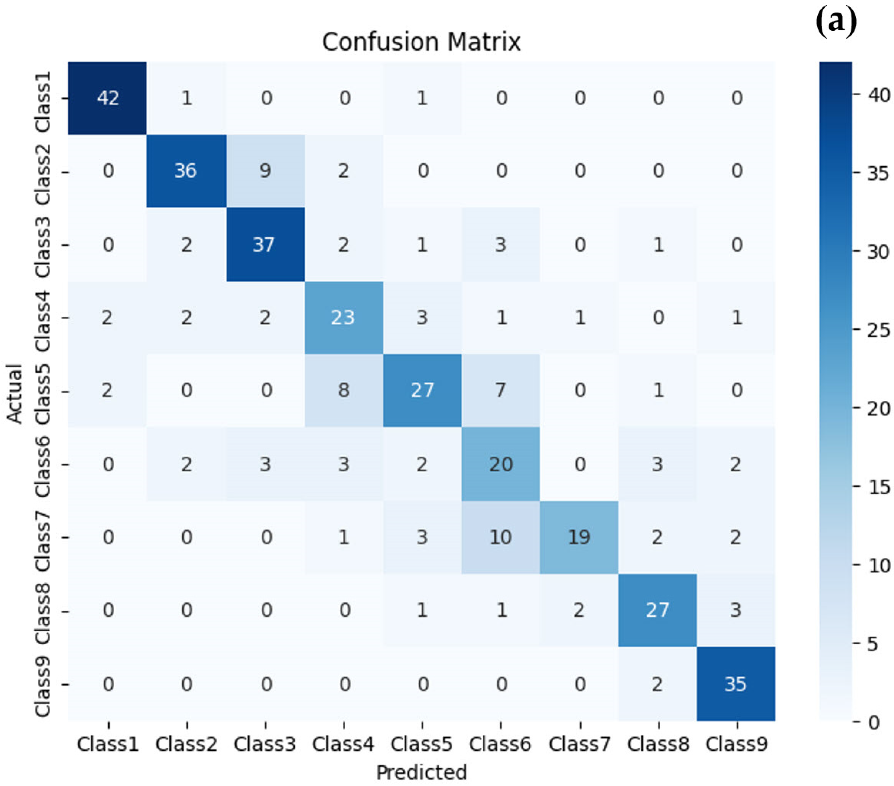
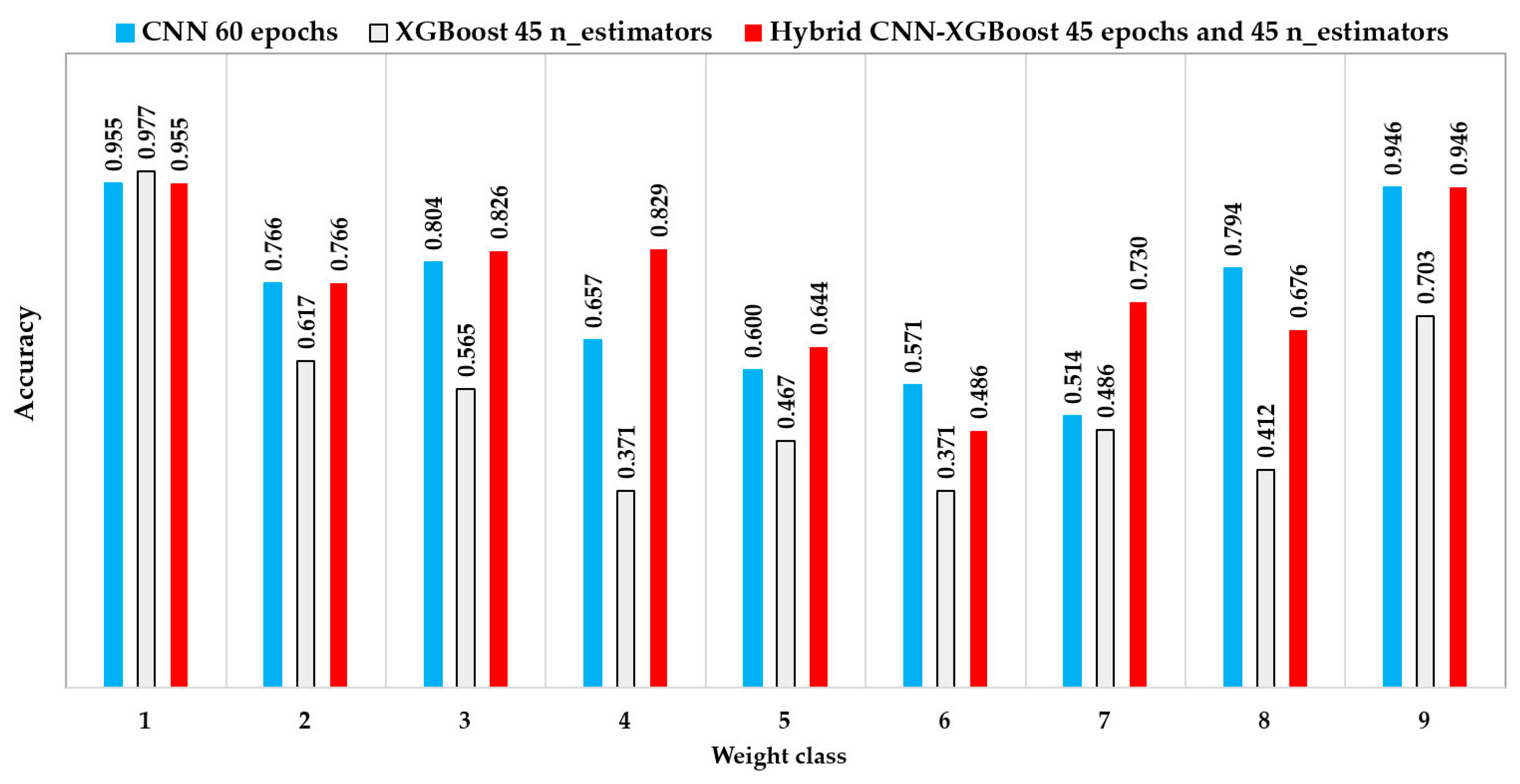
The confusion matrices for all three model types (Figure 3), derived from the best fine-tuning results, revealed consistent accuracy in predicting class 1 weight, accompanied by a notable decrease in accuracy for predicting weights in other classes. Figure 4 shows that the CNN model (60 epochs) revealed accuracy in weights prediction for classes 1–9 at the rate of 0.955, 0.766, 0.804, 0.657, 0.600, 0.571, 0.514, 0.794, and 0.946, respectively. Moreover, the XGBoost model (45 n_estimators) showed accuracies of 0.977, 0.617, 0.565, 0.371, 0.467, 0.371, 0.486, 0.412, and 0.703, respectively. In the meantime, the hybrid model CNN-XGBoost (with epochs and n_estimators of 45) achieved accuracies equivalent to 0.955, 0.766, 0.826, 0.829, 0.644, 0.486, 0.730, 0.676, and 0.946, respectively. These results highlighted the varying degrees of accuracy across different weight classes for each model.

4. Discussion

The average water quality parameters were considered suitable for tilapia culture based on the following criteria: DO concentration > 3 mg/L [35], Temp in the range of 26–32 °C, pH in the range of 6.5–8, ALK in the range of 10–400 [36], TAN < 1 mg/L [37], and Trans in a range that had no apparent negative impact on tilapia feeding behavior or growth. There was no published consensus among the specialized literature regarding the ideal Trans range.
Selecting an appropriate distance and period for using the UAV is essential and should remain fixed throughout the experiment. In our study, the distance between the UAV and the water surface was set at 3.5 m. This distance allowed the flight to cover the 5 × 5 m internal cage surface dimensions and the area around the cage. It was the closest distance that could be easily maintained, as the pilot could still see the UAV from the control point and was sufficiently above the water surface to avoid affecting fish behavior. Additionally, it increased the ground sample distance (GSD, measured in cm pixel−1) in the image, allowing for more effective image analysis [33,38,39]. The best time for taking images was reported to be in the morning, before the first feeding, to avoid any impact from sun glare. This, combined with tilapia normally having an average digestion time of 4–5 h before entering the empty stomach state, made the fish ready to eat the floating pellets about 1 h before feeding. This caused them to swim near the water surface.
In the evaluation of fish weight estimation, the Hybrid CNN-XGBoost model demonstrates higher accuracy compared to using standalone CNN and XGBoost models. This superiority arises from the ability of the Hybrid model to blend the strengths of the sub-models used together. CNNs excel in extracting hierarchical features from data through convolutional layers, effectively processing complex image patterns. On the other hand, XGBoost excels in handling tabular data and decision-making using boosted decision trees, making it adept at capturing non-linear relationships in the data. This proves beneficial in dealing with complex data patterns, especially in situations where the relationships between features are intricate and non-linear, as observed in this study. This result is supported by the studies conducted by Ren et al. [40] and Jiao et al. [24]. Moreover, the Hybrid CNN-XGBoost model runs fewer epochs for the CNN component compared to a standalone CNN model. This may be because the CNN component focuses on feature extraction, and the integration of XGBoost complements it, optimizing overall model performance. However, the accuracy of all models was low in classes 5–8. This could be because the farmer conducted partial harvesting, which altered the total number of fish in the cages and could have affected the accuracy of weight estimation using the models. Another finding from this study is that the hybrid model not only achieved the highest accuracy but also reduced the time required for weight estimation compared to using the standalone CNN. This reduction was approximately 11.81%.
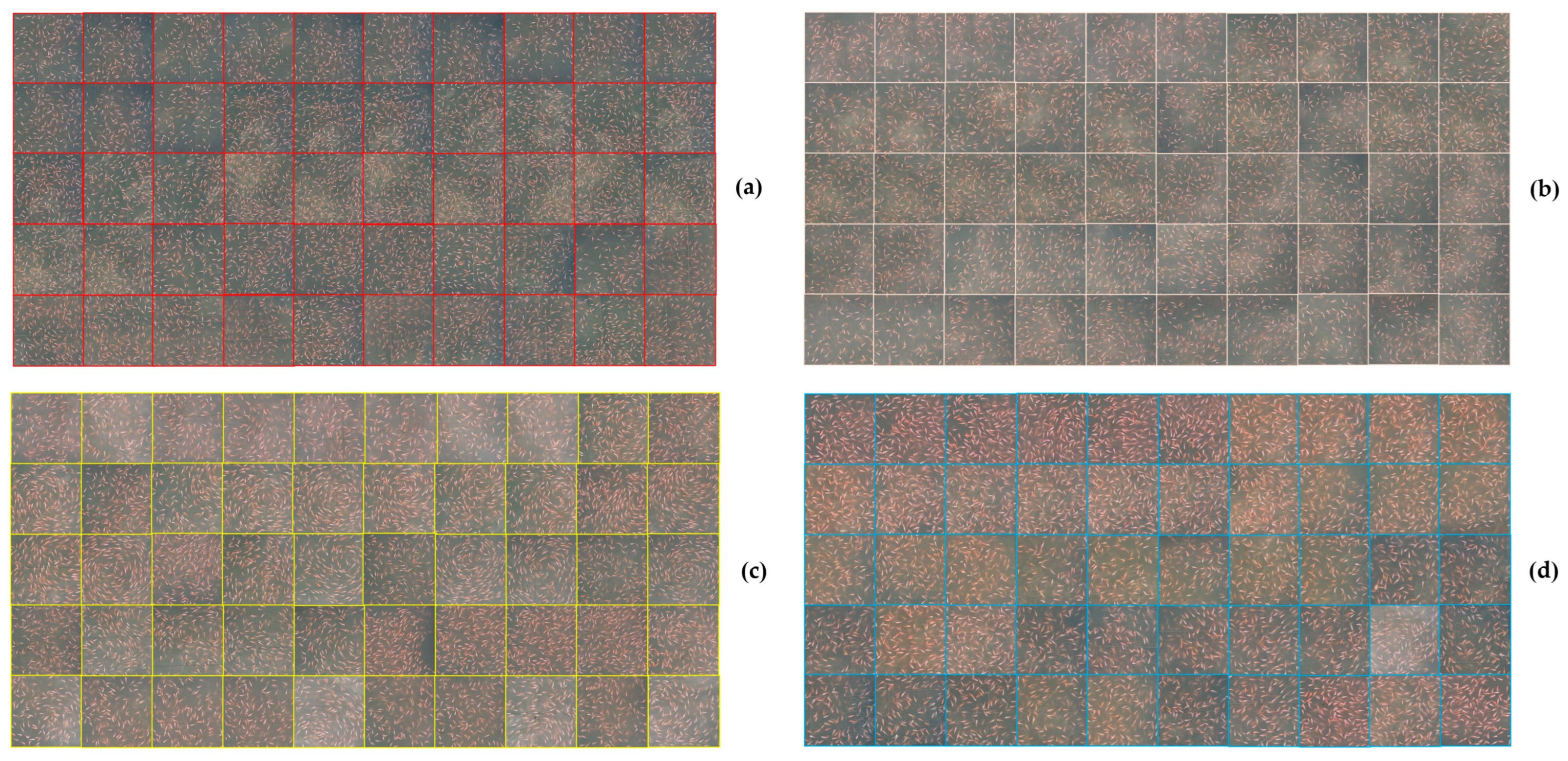
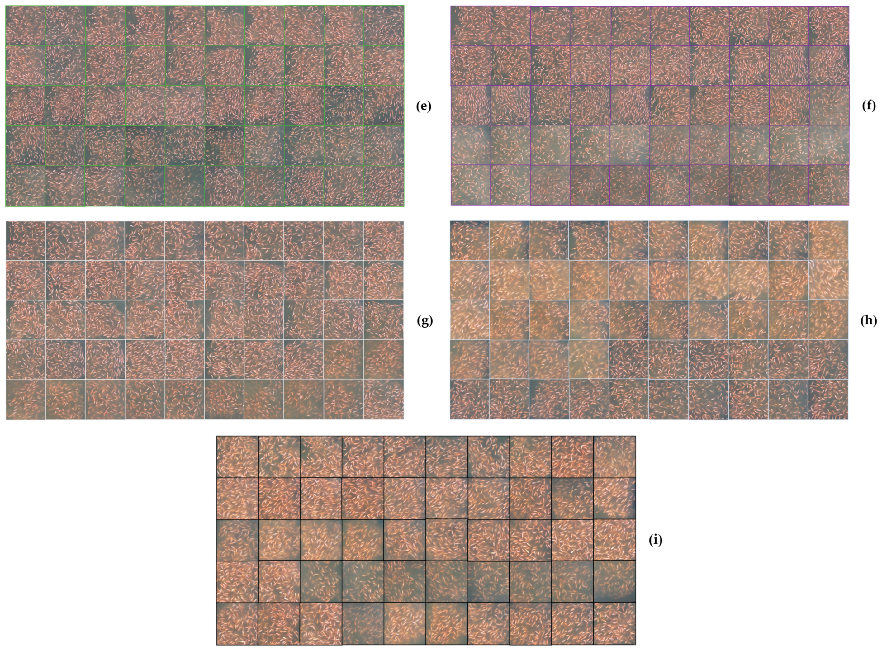
In the testing process, a comparison with previous studies that utilized other deep learning algorithms revealed that our experimental results (0.760 ± 0.019 or 76.00 ± 1.90% true class prediction) were less accurate. For instance, Konovalov et al. [15] applied a segmentation CNN model to estimate the mass of harvested Asian seabass (Lates calcarifer) in motionless specimens. The CNN prediction used the fish body to fit the mass area estimation models during validation. The single-factor model had a coefficient of determination (R2) value of 0.98, and the two-factor model had an R2 value of 0.98. Zhang et al. [41] used a principal component analysis calibration factor and a backpropagation neural network algorithm to estimate the weight of Crucian carp (Carassius carassius) under laboratory conditions (motionless specimens), achieving a testing R2 value of 0.90. Tengtrairat et al. [6] utilized a deep neural network (Mask R-CNN) with transfer learning for tilapia weight estimation in turbid water under laboratory conditions (individuals swimming freely in glass aquaria). Their proposed method produced experimental results with a mean absolute error of 42.54 g, an R2 of 0.70 (70% testing results), and an average weight error of 30.30 ± 23.09 g in a turbid water environment. Although our test results were less accurate than those conducted in laboratories due to uncontrollable field conditions, this study’s findings can be applied in the field. This variability contributes to diverse representations of fish across different sizes, as depicted in Figure 5.
To enhance accuracy, we recommend increasing the sample size of images and extending the data collection period to cover one year, enabling the observation of seasonal effects on the evaluation outcomes. Furthermore, incorporating image extraction is recommended, as studies indicate its potential to improve accuracy [42]. Our case study highlighted the potential of an affordable and mobile approach that combines UAV survey data with MVS to identify variations in the sizes of freely moving red tilapia within culture habitats. This methodology could serve as an alternative to prevailing techniques, which are often time-consuming. The conventional method typically involves randomly capturing and weighing fish, requiring 20–30 min per cage (around 20 fish/cage) and the efforts of two to four workers. Nevertheless, there remains a need for improving the accuracy percentage of the testing process in future research endeavors.
The current limitation of this study was the inability to measure fish size in real time. Next, a fish weight estimation program using UAV-captured images needs to be developed to provide real-time results.

5. Conclusions

The utilization of a UAV offers a solution for rapid and effortless image acquisition. These vehicles can be moved freely to capture images, rendering the process more cost-effective for scenarios involving extensive farming, as demonstrated in our study. In addition, this approach substantially reduces the time required for image acquisition. However, based on our study results, the Hybrid CNN-XGBoost model achieved accuracy levels of only 0.76, slightly below the common threshold of 0.90 frequently surpassed in most research studies. This discrepancy in accuracy can be attributed to the real-world nature of our study, where a multitude of environmental factors, ranging from fish characteristics to weather conditions and water quality, vary significantly and cannot be controlled uniformly or maintained consistently, as in laboratory settings. Therefore, to enhance the accuracy of the model in future implementations, we recommend increasing the number of images used, optimizing the hybrid model, or incorporating automated image extraction processes.

Author Contributions

Conceptualization, W.T. and R.J.; methodology, R.J., S.N., P.S. and W.M.; software, W.T., R.J. and P.S.; validation, W.T., R.J. and P.S.; formal analysis, W.T. and R.J.; investigation, W.T. and R.J.; resources, R.J. and W.M.; data curation, R.J. and P.S.; writing—original draft preparation, W.T. and R.J.; writing—review and editing, W.T. and R.J.; visualization, W.T. and R.J.; supervision, W.T.; project administration, R.J.; funding acquisition, R.J. and W.M. All authors have read and agreed to the published version of the manuscript.

Funding

This work (Grant No. RGNS 65-036) was supported by the Office of the Permanent Secretary, Ministry of Higher Education, Science, Research and Innovation (OPS MHESI), Thailand Science, Research and Innovation (TSRI), Fishbear Farm, and Kasetsart University, Bangkok, Thailand.

Data Availability Statement

The data presented in this study are available on request from the corresponding author.

Acknowledgments

The authors appreciate the assistance provided by staff at Fishbear Farm and aquacultural engineering laboratory. The authors acknowledge using ChatGPT (GPT-3.5, OpenAI) for text editing to improve the fluency of the English language in the preparation of this manuscript. The authors affirm that the original intent and meaning of the content remained unaltered during editing, and that ChatGPT had no involvement in shaping the intellectual content of this work. The authors assume full responsibility for upholding the integrity of the content presented in this study.

Conflicts of Interest

The authors declare no conflicts of interest.

References

  1. Food & Agricultural Organization. The State of World Fisheries and Aquaculture 2020; FAO: Rome, Italy, 2020; Available online: https://www.fao.org/documents/card/en/c/ca9229en (accessed on 28 September 2023).
  2. Dey, M.M.; Gupta, M.V. Socioeconomics of disseminating genetically improved Nile tilapia in Asia: An introduction. Aquac. Econ. Manag. 2000, 4, 5–11. [Google Scholar] [CrossRef]
  3. Ansari, F.A.; Nasr, M.; Guldhe, A.; Gupta, S.K.; Rawat, I.; Bux, F. Techno-economic feasibility of algal aquaculture via fish and biodiesel production pathways: A commercial-scale application. Sci. Total Environ. 2020, 704, 135259. [Google Scholar] [CrossRef] [PubMed]
  4. Sgnaulin, T.; Durigon, E.G.; Pinho, S.M.; Jerônimo, T.; de Alcantara Lopes, D.L.; Emerenciano, M.G.C. Nutrition of genetically improved farmed tilapia (GIFT) in biofloc technology system: Optimization of digestible protein and digestible energy levels during nursery phase. Aquaculture 2020, 521, 734998. [Google Scholar] [CrossRef]
  5. Pongthana, N.; Nguyen, N.H.; Ponzoni, R.W. Comparative performance of four red tilapia strains and their crosses in fresh- and saline water environments. Aquaculture 2010, 308, S109–S114. [Google Scholar] [CrossRef]
  6. Tengtrairat, N.; Woo, W.L.; Parathai, P.; Rinchumphu, D.; Chaichana, C. Non-intrusive fish weight estimation in Turbid water using deep learning and regression models. Sensors 2022, 22, 5161. [Google Scholar] [CrossRef] [PubMed]
  7. Zion, B. The use of computer vision technologies in aquaculture—A review. Comput. Electron. Agric. 2012, 88, 125–132. [Google Scholar] [CrossRef]
  8. Li, D.; Hao, Y.; Duan, Y. Nonintrusive methods for biomass estimation in aquaculture with emphasis on fish: A review. Rev. Aquac. 2019, 12, 1390–1411. [Google Scholar] [CrossRef]
  9. Rodríguez Sánchez, V.; Rodríguez-Ruiz, A.; Pérez-Arjona, I.; Encina-Encina, L. Horizontal target strength-size conversion equations for sea bass and gilt-head bream. Aquaculture 2018, 490, 178–184. [Google Scholar] [CrossRef]
  10. Petrell, R.J.; Shi, X.; Ward, R.K.; Naiberg, A.; Savage, C.R. Determining fish size and swimming speed in cages and tanks using simple video techniques. Aquac. Eng. 1997, 16, 63–84. [Google Scholar] [CrossRef]
  11. Silva, T.S.D.C.; Santos, L.D.D.; Silva, L.C.R.D.; Michelato, M.; Furuya, V.R.B.F.; Furuya, W.M. Length-weight relationship and prediction equations of body composition for growing-finishing cage-farmed Nile tilapia. Rev. Bras. Zootec. 2015, 44, 133–137. [Google Scholar] [CrossRef]
  12. Ashley, P.J. Fish welfare: Current issue in aquaculture. Appl. Anim. Behav. Sci. 2007, 104, 199–235. [Google Scholar] [CrossRef]
  13. Viazzi, S.; Van Hoestenberghe, S.; Goddeeris, B.M.; Berckmans, D. Automatic mass estimation of Jade perch Scortum barcoo by computer vision. Aquac. Eng. 2015, 64, 42–48. [Google Scholar] [CrossRef]
  14. Torisawa, S.; Kadota, M.; Komeyama, K.; Suzuki, K.; Takagi, T. A digital stereo-video camera system for three-dimensional monitoring of free-swimming Pacific bluefin tuna, Thunnus orientalis, cultured in a net cage. Aquat. Living. Resour. 2011, 24, 107–112. [Google Scholar] [CrossRef]
  15. Konovalov, D.A.; Saleh, A.; Domingos, J.A.; White, R.D.; Jerry, D.R. Estimating mass of harvested Asian seabass Lates calcarifer from Images. World J. Eng. Technol. 2018, 6, 15–23. [Google Scholar] [CrossRef]
  16. Gümüş, E.; Yılayaz, A.; Kanyılmaz, M.; Gümüş, B.; Balaban, M.O. Evaluation of body weight and color of cultured European catfish (Silurus glanis) and African catfish (Clarias gariepinus) using image analysis. Aquac. Eng. 2021, 93, 102147. [Google Scholar] [CrossRef]
  17. Taparhudee, W.; Jongjaraunsuk, R. Weight estimation of Nile tilapia (Oreochromis niloticus Linn.) using image analysis with and without fins and tail. J. Fish. Environ. 2023, 47, 19–32. [Google Scholar]
  18. LeCun, Y.; Bengio, Y.; Hinton, G. Deep learning. Nature 2015, 521, 436–444. [Google Scholar] [CrossRef]
  19. Jiang, X.; Wang, Y.; Liu, W.; Li, S.; Liu, J. CapsNet, CNN, FCN: Comparative performance evaluation for image classification. Int. J. Mach. Learn. 2019, 9, 840–848. [Google Scholar] [CrossRef]
  20. Goodwin, A.; Padmanabhan, S.; Hira, S.; Glancey, M.; Slinowsky, M.; Immidisetti, R.; Scavo, L.; Brey, J.; Sudhakar, B.M.M.S.; Ford, T.; et al. Mosquito species identification using convolutional neural networks with a multitiered ensemble model for novel species detection. Sci. Rep. 2021, 11, 13656. [Google Scholar] [CrossRef]
  21. Meckbach, C.; Tiesmeyer, V.; Traulsen, I. A promising approach towards precise animal weight monitoring using convolutional neural networks. Comput. Electron. Agric. 2021, 183, 106056. [Google Scholar] [CrossRef]
  22. Rančić, K.; Blagojević, B.; Bezdan, A.; Ivošević, B.; Tubić, B.; Vranešević, M.; Pejak, B.; Crnojević, V.; Marko, O. Animal detection and counting from UAV images using convolutional neural networks. Drone 2023, 7, 179. [Google Scholar] [CrossRef]
  23. Chen, T.Q.; Guestrin, C. XGboost: A scalable tree boosting system. In Proceedings of the 22nd ACM SIGKDD International Conference on Knowledge Discovery and Data Mining, San Francisco, CA, USA, 13–17 August 2016; pp. 785–794. [Google Scholar]
  24. Jiao, W.; Hao, X.; Qin, C. The image classification method with CNN-XGBoost model based on adaptive particle swarm optimization. Information 2021, 12, 156. [Google Scholar] [CrossRef]
  25. Tseng, C.J.; Tang, C. An optimized XGBoost techinique for accurate brain tumor detection using feature selection and image segmentation. Healthc. Anal. 2023, 4, 100217. [Google Scholar] [CrossRef]
  26. Kwenda, C.; Gwetu, M.V.; Fonou-Dombeu, J.V. Forest image classification based on deep learning and XGBoost algorithm. In Lecture Notes in Computer Science; Springer: Cham, Switzerland, 2023. [Google Scholar]
  27. Hamzaoui, M.; Aoueileyine, M.O.E.; Romdhani, L.; Bouallegue, R. Optimizing XGBoost performance for fish weight prediction through parameter pre-selection. Fishes 2023, 8, 505. [Google Scholar] [CrossRef]
  28. Nurdin, Z.; Hidayat, T.; Irvanizam, I. Performance comparison of hybrid CNN-XGBoost and CNN-LightGBM methods in pneumonia detection. In Proceedings of the International Conference on Electrical Engineering and Informatics (ICELTICs), Banda Aceh, Indonesia, 27–28 September 2022; pp. 31–36. [Google Scholar]
  29. Zivkovic, M.; Bacanin, N.; Antonijevic, M.; Nikolic, B.; Kvascev, G.; Marjanovic, M.; Savanovic, N. Hybrid CNN and XGBoost model tuned by modified arithmetic optimization algorithm for COVID-19 early diagnostics from X-ray images. Electronics 2022, 11, 3798. [Google Scholar] [CrossRef]
  30. Murugan, D.; Garg, A.; Singh, D. Development of an adaptive approach for precision agriculture monitoring with drone and satellite data. IEEE J. Sel. Top. Appl. Earth Obs. Remote Sens. 2017, 10, 5322–5328. [Google Scholar] [CrossRef]
  31. Shahi, T.B.; Xu, C.Y.; Neupane, A.; Guo, W. Recent advances in crop disease detection using UAV and deep learning techniques. Remote Sens. 2023, 15, 2450. [Google Scholar] [CrossRef]
  32. Fong, V.; Hoffmann, S.L.; Pate, J.H. Using drones to assess volitional swimming kinematics of manta ray behaviors in the wild. Drones 2022, 6, 111. [Google Scholar] [CrossRef]
  33. Taparhudee, W.; Jongjaraunsuk, R.; Nimitkul, S.; Mathurossuwan, W. Application of unmanned aerial vehicle (UAV) with area image analysis of red tilapia weight estimation in river-based cage culture. J. Fish. Environ. 2023, 47, 119–130. [Google Scholar]
  34. APHA. Standard Methods for the Examination of Water and Wastewater, 20th ed.; American Public Health Association, American Water Works Association, Water Environment Federation: Washington, DC, USA, 2005. [Google Scholar]
  35. Tran-Duy, A.; Van Dam, A.A.; Schrama, J.W. Feed intake, growth and metabolism of Nile tilapia (Oreochromis niloticus) in relation to dissolved oxygen concentration. Aquac. Res. 2012, 43, 730–744. [Google Scholar] [CrossRef]
  36. Lawson, T.B. Fundamentals of Aquacultural Engineering; Chapman & Hall: New York, NY, USA, 1995. [Google Scholar]
  37. Sriyasak, P.; Chitmanat, C.; Whangchai, N.; Promya, J.; Lebel, L. Effect of water de-stratification on dissolved oxygen and ammonia in tilapia ponds in Northern Thailand. Int. Aquat. Res. 2012, 7, 287–299. [Google Scholar] [CrossRef]
  38. Wallace, L.; Lucieer, A.; Watson, C.; Turner, D. Development of a UAV-LiDAR system with application to forest inventory. Remote Sens. 2012, 4, 1519–1543. [Google Scholar] [CrossRef]
  39. Seifert, E.; Seifert, S.; Vogt, H.; Drew, D.; Aardt, J.V.; Kunneke, A.; Seifert, T. Influence of drone altitude, image overlap, and optical sensor resolution on multi-view reconstruction of forest images. Remote Sens. 2019, 11, 1252. [Google Scholar] [CrossRef]
  40. Ren, X.; Guo, H.; Li, S.; Wang, S.; Li, J. A Novel image classification method with CNN-XGBoost Model. In Digital Forensics and Watermarking, Proceedings of the 6th International Workshop, IWDW 2017, Magdeburg, Germany, 23–25 August 2017; Lecture Notes in Computer Science; Kraetzer, C., Shi, Y.Q., Dittmann, J., Kim, H., Eds.; Springer: Cham, Switzerland, 2017; Volume 10431. [Google Scholar]
  41. Zhang, J.; Zhuang, Y.; Ji, H.; Teng, G. Pig weight and body size estimation using a multiple output regression convolutional neural network: A fast and fully automatic method. Sensor 2021, 21, 3218. [Google Scholar] [CrossRef]
  42. Suwannasing, P.; Jongjaraunsuk, R.; Yoonpundh, R.; Taparhudee, W. A comparison of Image segmentation and image non-segmentation to classify average weight of red tilapia using machine learning techniques (Thai). Burapha Sci. J. 2023, 28, 208–222. [Google Scholar]
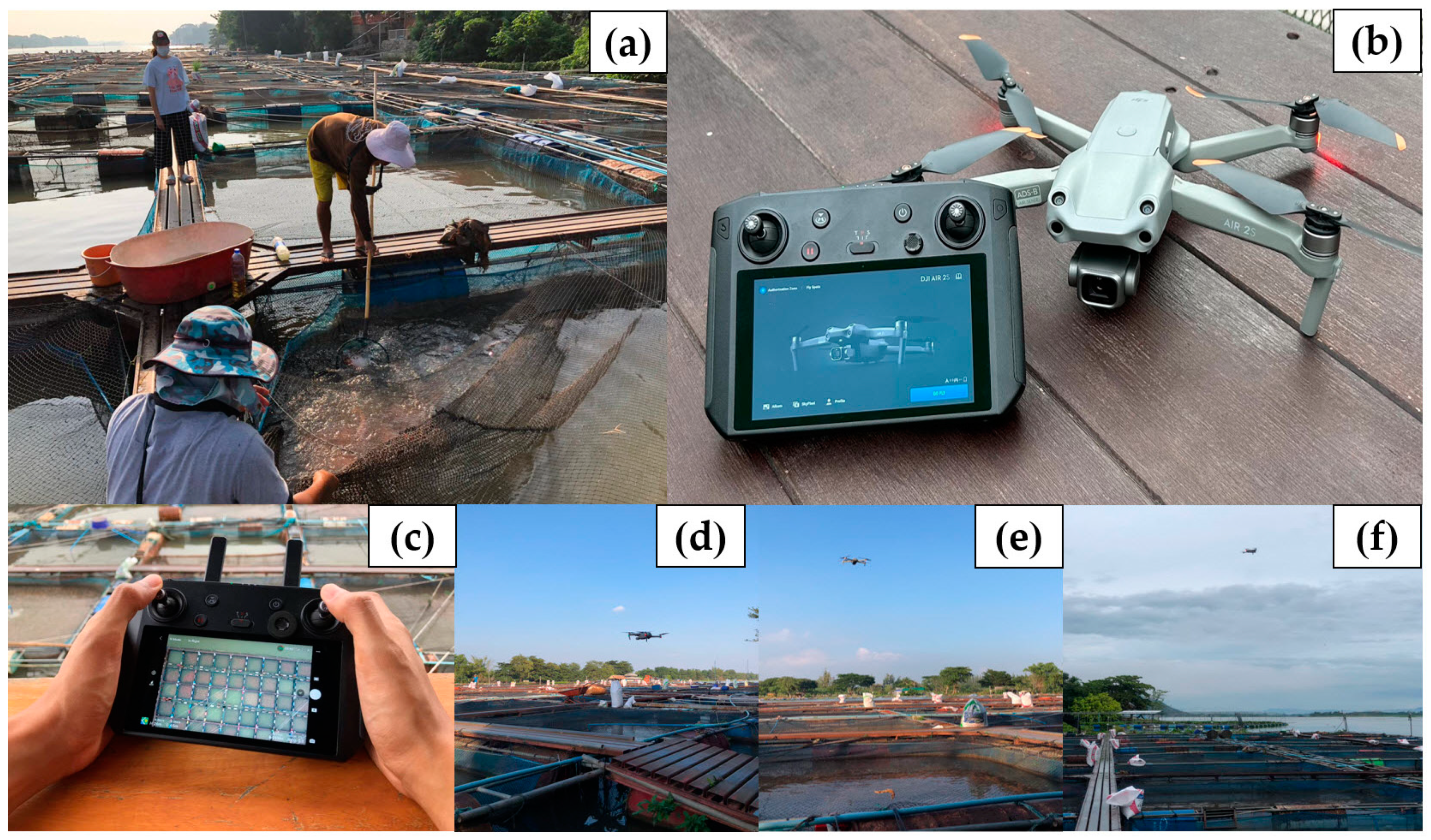
Figure 1. Twenty fish in each cage were randomly selected and weighed using a digital scale 1 day before the UAV flight (a); UAV, DJI Air 2S (Mavic) (b); DJI Smart Controller (c); UAV taking off from the landing station (d); and UAV flying over fish cages (e,f).
Agriengineering 06 00070 g001
Figure 2. Example of image used after preprocessing.
Agriengineering 06 00070 g002
Figure 3. Details of confusion matrices for the testing results of weight classification using CNN with 60 epochs (a), XGBoost with 45 n_estimators (b), and Hybrid CNN-XGBoost with 45 epochs and 45 n_estimators (c).
Agriengineering 06 00070 g003aAgriengineering 06 00070 g003b
Figure 4. Details of the average accuracy for fish weight prediction in each class obtained from the confusion matrices of the 3 best fine-tuning models: CNN with 60 epochs, XGBoost with 45 n_estimators, and Hybrid CNN-XGBoost with 45 epochs and 45 n_estimators.
Agriengineering 06 00070 g004
Figure 5. Fifty sample images from a set of four hundred images per class used in the analysis, where (ai) represent sample fish images in classes 1 through 9, respectively.
Agriengineering 06 00070 g005aAgriengineering 06 00070 g005b
Table 1. Specifications of DJI Air 2S (Mavic).
SpecificationValue and Description
Flight time34 min
Max service ceiling above sea level5000 m
Transmission systemOcuSync 2.0
Weight595 g
Folded size180 × 97 × 77 mm (length × width × height)
Max speed6 m/s (standard mode)
Maximum wind speed resistance10.7 m/s
Obstacle avoidance3-Direction cameras and IR
Special features4 K/60, HDR, 48 MP Photos
Phone chargingAvailable
Takeoff and landing lightAvailable
Internal storage8 GB
Note: OcuSync 2.0 is a transmission system developed by DJI, the manufacturer of the DJI Air 2S (Mavic). It is designed to provide a stable and reliable communication link between the UAV and its remote controller, as well as between the UAV and any connected devices such as smartphones or tablets. “IR” stands for infrared, “HDR” stands for high dynamic range, and “MP” stands for megapixels.
Table 2. Images captured during each UAV flight.
FlightDateNumber of CagesNumber of Images/CagesTotal Number of Images
122 January 2023850400
23 February 2023850400
318 February 2023850400
44 March 2023850400
517 March 2023850400
61 April 2023850400
722 April 2023850400
86 May 2023850400
920 May 2023850400
3600
Table 3. Developed structures of CNN, XGBoost, and Hybrid CNN-XGBoost models.
ModelStructure
CNN# Define the CNN model
Model = tf.keras.sequential([
Tf.keras.layers.conv2D (32, (3, 3), input_shape = (64, 64, 1), activation = ‘relu’),
Tf.keras.layers.maxpooling2D (pool_size = (2, 2)),
Tf.keras.layers.conv2D (64, (3, 3), activation = ‘relu’),
Tf.keras.layers.maxpooling2D (pool_size = (2, 2)),
Tf.keras.layers.flatten(),
Tf.keras.layers.dense (64, activation = ‘relu’),
Tf.keras.layers.dense (len(classes), activation = ‘softmax’)
])
# Compile the model
Model.compile (optimizer = ‘adam’, loss = ‘sparse_categorical_crossentropy’, metrics = [‘accuracy’])
# Train the model
History = model.fit (x_train, y_train, epochs = fine-tuned, validation_data = (x_val, y_val))
XGBoost# Define the XGBoost model
Model = xgb.xgbClassifier (objective = ‘multi:softmax’, num_class = len (classes), eval_metric = ‘mlogloss’, n_estimators = fine-tuned)
# Train the model
Model.fit (x_train, y_train)
CNN-XGBoost# Define the CNN model
# Extract features using the CNN model
CNN_features _train = CNN_model.predict (x_train)
CNN_features_val = CNN_model.predict (x_val)
CNN_features_test = CNN_model.predict (x_test)
# Train the CNN model (epochs = fine-tuned)
# Combine CNN features with original features
X_train_combined = np. concatenate ((x_train.reshape ((x_train.shape [0], −1)),
CNN_features_train)), axis = 1)
X_val_combined = np. concatenate ((x_val.reshape ((x_val.shape [0], −1)),
CNN_features_val), axis = 1)
X_test_combined = np. concatenate ((x_test.reshape ((x_test.shape [0], −1)),
CNN_features_test), axis = 1)
# Define the XGBoost model (n_estimators = fine-tuned)
# Train the model
Model.fit (x_train_combined, y_train)
Table 4. Details of 9 UAV flights, including fish weight range (minimum–maximum), water quality, and wind speed (mean ± SD).
Weight ClassFish Weight (g/Fish)DO (mg/L)Temp (°C)pHALK (mg/L)TAN (mg/L)Trans
(cm)
Wind Speed (m/s)
1119.38–170.284.26 ± 0.0425.90 ± 0.007.47 ± 0.01122.34 ± 6.130.09 ± 0.0170 ± 01.32 ± 0.04
2180.65–237.193.73 ± 0.0725.20 ± 0.007.44 ± 0.00126.00 ± 5.660.10 ± 0.0280 ± 00.89 ± 0.07
3234.33–310.313.80 ± 0.0926.20 ± 0.007.46 ± 0.00112.00 ± 2.830.12 ± 0.0370 ± 01.26 ± 0.08
4308.76–391.244.43 ± 0.1026.05 ± 0.217.52 ± 0.01110.00 ± 1.410.11 ± 0.0470 ± 01.06 ± 0.47
5404.07–496.413.95 ± 0.1127.13 ± 0.047.53 ± 0.01114.34 ± 3.300.10 ± 0.03100 ± 00.66 ± 0.11
6474.59–568.173.48 ± 0.0828.35 ± 0.217.53 ± 0.01122.00 ± 2.830.15 ± 0.0190 ± 00.78 ± 0.01
7564.53–662.613.66 ± 0.0829.27 ± 0.047.52 ± 0.01109.43 ± 4.850.17 ± 0.0298 ± 51.98 ± 0.17
8625.92–741.063.40 ± 0.1929.69 ± 0.057.59 ± 0.10105.67 ± 10.840.20 ± 0.0390 ± 00.81 ± 0.34
9695.91–830.293.82 ± 0.2029.60 ± 0.427.60 ± 0.02107.00 ± 4.240.20 ± 0.04105 ± 02.27 ± 0.77
Note: Dates of sample collection flights for each class are shown in Table 2.
Table 5. Performance comparison of CNN, XGBoost, and Hybrid CNN-XGBoost.
ModelAdjustedAccuracyPrecisionRecallF1 ScoreProcessing Time/Image
CNN10 epochs0.520 ± 0.0370.542 ± 0.0380.506 ± 0.0340.490 ± 0.0510.840 s
15 epochs0.544 ± 0.0550.558 ± 0.0630.538 ± 0.0540.516 ± 0.0630.920 s
20 epochs0.620 ± 0.0420.628 ± 0.0510.614 ± 0.0450.608 ± 0.0460.980 s
25 epochs0.666 ± 0.0430.692 ± 0.0340.662 ± 0.0480.656 ± 0.0431.120 s
30 epochs0.702 ± 0.0360.716 ± 0.0380.698 ± 0.0330.694 ± 0.0361.280 s
35 epochs0.692 ± 0.0220.706 ± 0.0210.684 ± 0.0260.680 ± 0.0251.560 s
40 epochs0.710 ± 0.0270.720 ± 0.0250.708 ± 0.0290.708 ± 0.0291.660 s
45 epochs0.720 ± 0.0290.728 ± 0.0330.716 ± 0.0340.716 ± 0.0321.900 s
50 epochs0.678 ± 0.0450.688 ± 0.0430.674 ± 0.0440.670 ± 0.0432.000 s
55 epochs0.730 ± 0.0070.730 ± 0.0160.722 ± 0.0110.720 ± 0.0072.260 s
60 epochs0.748 ± 0.0190.750 ± 0.0190.740 ± 0.0140.740 ± 0.0192.540 s
65 epochs0.742 ± 0.0160.748 ± 0.0130.738 ± 0.0180.738 ± 0.0182.880 s
70 epochs0.730 ± 0.0400.736 ± 0.0290.728 ± 0.0340.724 ± 0.0372.980 s
XGBoost10 n_estimators0.480 ± 0.0000.470 ± 0.0000.470 ± 0.0000.470 ± 0.0000.420 s
15 n_estimators0.500 ± 0.0000.490 ± 0.0000.490 ± 0.0000.490 ± 0.0000.440 s
20 n_estimators0.510 ± 0.0000.500 ± 0.0000.500 ± 0.0000.500 ± 0.0000.500 s
25 n_estimators0.530 ± 0.0000.520 ± 0.0000.520 ± 0.0000.520 ± 0.0000.560 s
30 n_estimators0.530 ± 0.0000.520 ± 0.0000.510 ± 0.0000.510 ± 0.0000.600 s
35 n_estimators0.540 ± 0.0000.530 ± 0.0000.520 ± 0.0000.520 ± 0.0000.660 s
40 n_estimators0.550 ± 0.0000.540 ± 0.0000.540 ± 0.0000.540 ± 0.0000.700 s
45 n_estimators0.560 ± 0.0000.550 ± 0.0000.550 ± 0.0000.550 ± 0.0000.720 s
50 n_estimators0.560 ± 0.0000.550 ± 0.0000.550 ± 0.0000.540 ± 0.0000.760 s
55 n_estimators0.560 ± 0.0000.540 ± 0.0000.540 ± 0.0000.540 ± 0.0000.780 s
60 n_estimators0.560 ± 0.0000.550 ± 0.0000.550 ± 0.0000.540 ± 0.0000.820 s
Hybrid CNN-XGBoost10 epochs/10 n_estimators0.722 ± 0.0300.716 ± 0.0310.716 ± 0.0310.714 ± 0.0290.920 s
15 epochs/15 n_estimators0.720 ± 0.0240.714 ± 0.0210.712 ± 0.0220.712 ± 0.0221.040 s
20 epochs/20 n_estimators0.750 ± 0.0190.750 ± 0.0190.744 ± 0.0170.740 ± 0.0191.220 s
25 epochs/25 n_estimators0.734 ± 0.0210.736 ± 0.0230.728 ± 0.0200.726 ± 0.0181.540 s
30 epochs/30 n_estimators0.746 ± 0.0190.744 ± 0.0170.738 ± 0.0220.740 ± 0.0211.740 s
35 epochs/35 n_estimators0.758 ± 0.0230.754 ± 0.0220.750 ± 0.0230.750 ± 0.0231.800 s
40 epochs/40 n_estimators0.748 ± 0.0110.752 ± 0.0150.742 ± 0.0150.742 ± 0.0151.980 s
45 epochs/45 n_estimators0.760 ± 0.0190.762 ± 0.0190.754 ± 0.0190.752 ± 0.0192.240 s
50 epochs/50 n_estimators0.746 ± 0.0270.746 ± 0.0270.740 ± 0.0240.742 ± 0.0262.440 s
55 epochs/55 n_estimators0.734 ± 0.0210.736 ± 0.0220.728 ± 0.0220.726 ± 0.0222.480 s
60 epochs/60 n_estimators0.746 ± 0.0170.750 ± 0.0210.744 ± 0.0170.744 ± 0.0172.740 s
Note: Bold indicates the best-performing model for precise estimation of red tilapia weight class.
Disclaimer/Publisher’s Note: The statements, opinions and data contained in all publications are solely those of the individual author(s) and contributor(s) and not of MDPI and/or the editor(s). MDPI and/or the editor(s) disclaim responsibility for any injury to people or property resulting from any ideas, methods, instructions or products referred to in the content.