Hierarchically Coupled Ornstein–Uhlenbeck Processes for Transient Anomalous Diffusion


Department of Mathematics and Statistics, Washington State University, Pullman, WA 99164, USA
*
Author to whom correspondence should be addressed.
Physics 2024, 6(2), 645-658; https://doi.org/10.3390/physics6020042
Submission received: 15 January 2024
/
Revised: 6 March 2024
/
Accepted: 9 March 2024
/
Published: 24 April 2024
(This article belongs to the Section Statistical Physics and Nonlinear Phenomena)
Abstract
:The nonlinear dependence of the mean-squared displacement (MSD) on time is a common characteristic of particle transport in complex environments. Frequently, this anomalous behavior only occurs transiently before the particle reaches a terminal Fickian diffusion. This study shows that a system of hierarchically coupled Ornstein–Uhlenbeck equations is able to describe both transient subdiffusion and transient superdiffusion dynamics, as well as their sequential combinations. To validate the model, five distinct experimental, molecular dynamics simulation, and theoretical studies are successfully described by the model. The comparison includes the transport of particles in random optical fields, supercooled liquids, bedrock, soft colloidal suspensions, and phonons in solids. The model’s broad applicability makes it a convenient tool for interpreting the MSD profiles of particles exhibiting transient anomalous diffusion.
1. Introduction
Standard Brownian motion (BM) theory, as established by Albert Einstein, Marian Smoluchowski, and Paul Langevin in the early last century, cannot adequately describe the transport properties of active or passive particles in complex environments [1,2,3,4,5,6]. One of the primary discrepancies arises from the anomalous diffusion patterns frequently observed in these systems. In these instances, the mean-squared displacement (MSD) of the particles (tracers) does not increase linearly with time, t, as predicted by standard BM (Fickian diffusion). Instead, it is observed that
where the exponent deviates from unity. In cases where , the particle diffuses slower than BM (subdiffusion), whereas, for cases with , the diffusion is faster (superdiffusion). Quite often, the anomalous behavior is only transient, meaning the MSD is diffusive or ballistic at relatively short times, then it transitions to anomalous diffusion (subdiffusion or superdiffusion) and entails entirely Fickian diffusion at longer time scales. Anomalous diffusion in passive BM has been observed in soft biological systems [7,8,9,10,11,12], supercooled and ionic liquids [13,14,15,16,17,18], granular and glassy materials [19,20,21,22,23,24,25,26,27], colloidal suspensions [28,29], as well as diffusion under random external fields [30,31]. In active motion, anomalous diffusion has been reported in cell motion [32], chemically powered nanomotors [33], and even mammal movement [34].
Theoretical frameworks often employ continuous-time random walks (CTRWs) as a general method for modeling anomalous diffusion [17,35,36,37,38,39,40]. This stochastic process is based on a random walk (RW) that moves in independent directions with steps and waiting times drawn from specific distributions. Transient anomalous diffusion becomes feasible when employing truncated power law distributions [41]. The continuous counterparts of CTRW, represented by fractional diffusion and fractional Fokker–Planck equations, are also regularly implemented to describe transport properties in complex environments [42,43]. Fractional BM is another established stochastic process that effectively characterizes anomalous diffusion [44,45]. Notably, fractional BM captures Equation (1) while being a Gaussian process. Studies based on the Langevin equation and its generalization, whether involving scaled Brownian motion, fractional derivatives, or with or without tempered memory kernels, form a major category for modeling anomalous diffusion [46,47,48,49,50,51,52,53,54,55,56].
This study demonstrates that a mathematical model based on a hierarchical implementation of the kinetic theory [57] effectively captures various aspects of transient anomalous diffusion. This model can be mathematically formulated either as an RW coupled to n independent noise sources or by a system of hierarchically coupled Ornstein–Uhlenbeck (OU) processes. Following the results in [57,58], it is shown here that, for , the model can capture a wide range of transient super- and subdiffusive dynamics, regardless of whether the initial behavior is ballistic or diffusive. The analytical and numerical results are in exceptional qualitative agreement with a broad range of experimental, molecular dynamics (MD) simulation, and other numerical and theoretical studies. Interestingly, by incorporating more than two noise sources, the model describes a series of alternating super- and subdiffusion dynamics, a result that has been observed in soft colloids and cell motion in embryonic tissue [28,59]. The model predictions were validated by comparing them to five experimental and theoretical studies [28,30,60,61,62]. Similar to the aforementioned theoretical studies, the present model is also characterized by its simplicity since it admits analytical solutions. Besides, its potential to also describe both transient superdiffusion and subdiffusion, as well as multiple layers of different diffusion phases, offers a convenient description of transient anomalous diffusion. It should be noted that active OU models are capable of modeling transient superdiffusion [63,64,65,66]. As we show below, such models qualitatively agree with our approach when and .
The paper is organised as follows. The model recently proposed in Ref. [57] is briefly discussed in Section 2. Section 3 describes four different cases of transient anomalous diffusion that can be captured by the system of hierarchically coupled OU equations. Section 4 directly compares the model predictions with experimental, MD simulation, and theoretical studies. Lastly, Section 5 briefly summarizes the study.
2. Hierarchically Coupled OU Equations
Consider a particle moving through a complex one-dimensional environment characterized by the presence of n independent white noise sources, , where , denote the BM paths, denote the diffusivities, and are independent Wiener increments. In a recent study [57], it was suggested that the position, , of the particle can be described by the following equation:
where each is a positive constant and represents the relaxation rates at each noise level. Any state with is described by the same equation as if only the first i noise sources were considered. Since the jth state affects the ith state only if , Equation (2) describes a series of hierarchically coupled processes. By introducing the change of variables:
Equation (2) reduces to a system of hierarchically coupled OU processes:
where . A similar change of variables has also been used in Ref. [63]. Equation (4) admits an analytical solution that describes a non-equilibrium stationary state distribution [57]. Therefore, the particle’s velocity, as expressed by Equation (2):
is well-defined and also exhibits a stationary distribution.
In the special case of , both the Langevin equation and Equation (4) have the same solution after suitable parameter rescaling, as shown in Ref. [57]. However, the key difference lies in the way they address random fluctuations in the equations of motion. The Langevin equation introduces random fluctuations as stochastic forces, while this model assumes that the particle is trapped around a BM path () by a linear force of constant . Thus, in the long enough term, the particle follows the BM with diffusivity . In line with the kinetic theory, Equation (2) describes a ballistic motion at quite short times, and after a characteristic timescale of , the motion becomes diffusive [57]. The resulting motion matches the BM of the Langevin equation. Thus, for , one can add external force fields to perform standard Langevin dynamics simulations for the model. However, here, we argue that the introduction of extra noise sources () in Equation (2) can mimic both sub- and superdiffusion. Specifically, if the particle is subsequently influenced by a second noise source, one can similarly assume that the Brownian particle is trapped around an additional BM path () with its own distinct elastic constant, . In this case, the tracer is still influenced by the first noise source, but eventually, follows the trajectory of . If , then the particle significantly slows down, thus mimicking the structural or dynamics heterogeneity traps that are observed in nature. The generalization for any number of noise sources, n, leads to Equation (2). A more detailed interpretation of the proposed model and its connection to the kinetic theory can be found in Ref. [57].
In what follows, the vector is used to define the diffusivities and relaxation parameters when necessary.
3. Transient Anomalous Diffusion
Equation (2) was initially developed to study transient subdiffusion dynamics [57]. However, it can also effectively model transient superdiffusion, as well as more complex dynamics involving multiple anomalous diffusion regimes. The standard way to characterize diffusion is through the MSD of the tracer’s position from the initial condition, i.e., . Here, the MSD is defined as , where denotes the ensemble average. The computation can be achieved by solving Equation (4) and, then, using Equation (3) to compute . The can be computed using Ito’s integral properties.
This Section presents four different MSD profiles that the model can describe. The profiles have been reported in either experimental, MD simulation, numerical or theoretical studies. A comparison of our model with the studies listed is given in Section 3.1, Section 3.2, Section 3.3 and Section 3.4 just below.
3.1. Case A: Ballistic to Diffusive Crossover
By utilizing the analytical solution of Equation (4) [57], it is straightforward to show that, when , the MSD is expressed as
The asymptotic analysis of this equation demonstrates the transition from ballistic to diffusive behavior:
It is noteworthy that, when , Equation (2) produces results consistent with Langevin dynamics by setting and , where m is the mass of the tracer, represents the fluid friction, while and T are Boltzmann’s constant and the temperature of the system, respectively. This ballistic to diffusive crossover can also be described by active OU models.
3.2. Case B: Ballistic to Anomalous to Fickian Diffusion
Two interesting cases are worth noting. First, Equation (8) exhibits the following asymptotic behavior:
Second, when , the MSDs for and are approximately the same, i.e.,
With these assumptions, Equations (9) and (10) suggest that the particle always moves ballistically for a quite short time, and its subsequent diffusive behavior is controlled by the ratio . Specifically, the particle motion undergoes a transition from transient sub-diffusion when to normal diffusion when and transient superdiffusion when .
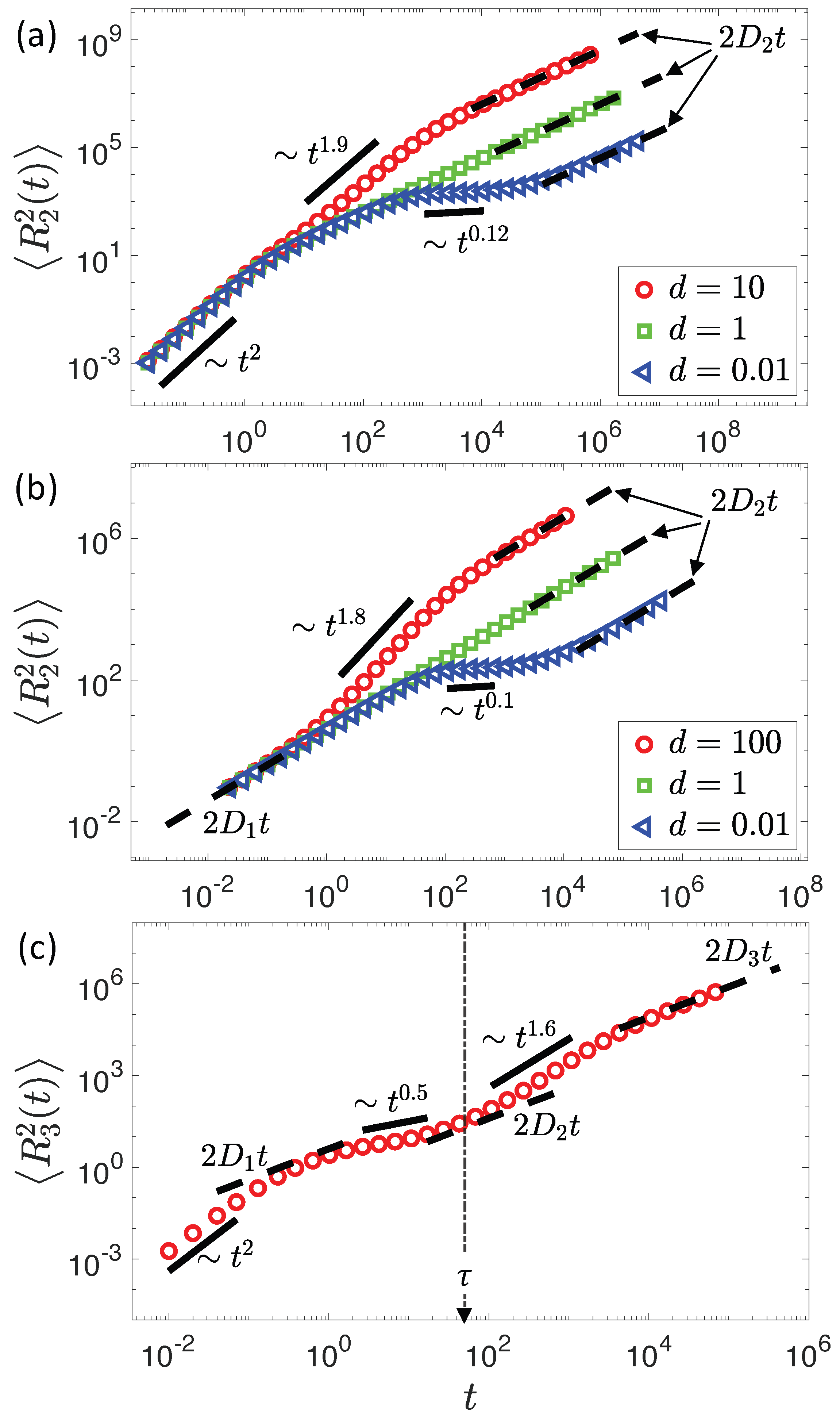
This behavior is illustrated in Figure 1a. In all three cases, the system begins with ballistic motion and ends with normal diffusion with diffusivity . The transient subdiffusive dynamics for is shown in Figure 1a with blue triangles. For this parameter set, the exponent of the transient subdiffusion is . The transient superdiffusion is shown with red circles, corresponding to . Here, the superdiffusion occurs with an exponent . Additionally, for , one has , demonstrating a direct transition from ballistic to diffusive dynamics.
3.3. Case C: Fickian to Anomalous Back to Fickian Diffusion
One can show that the MSD has the following asymptotic behavior for any value of :
Furthermore, when , the diffusion becomes Fickian, i.e.,
Similar to case B, Equations (12) and (13) provide two essential insights into the particle’s dynamics. First, the motion is always diffusive for relatively short and long enough times. Second, the nature of the motion between the two diffusive regimes is also controlled by the ratio . Specifically, the particle experiences transient subdiffusion when , normal diffusion when , and transient superdiffusion when . This transition is demonstrated in Figure 1b.
3.4. Case D: Multilayered Transient Anomalous Diffusion
For , the MSD is
where
and for , . Here, represent the entries of the equilibrium covariance matrix that is given in Appendix A.2. It must be underlined that the analysis is restricted to the cases with . This condition enables the particle to interact with each noise source in a sequential manner. Thus, the relative order of , , and ultimately determines the nature of the transient anomalous diffusion.
Let us discuss a typical case of with , as shown in Figure 1c. It is apparent that the MSD profile reveals a pattern of alternating diffusive behaviors. The motion exhibits ballistic behavior at relatively short times, followed by a brief period of normal diffusion (). Subsequently, it undergoes subdiffusion with before entering another brief diffusive phase (). Afterwards, the MSD becomes superdiffusive with and returns to a final diffusive regime () after a longer period of time.
The entire MSD profile can be viewed as a combination of cases B and C discussed above. Notably, there is a characteristic time that separates two distinct transient anomalous dynamics. For , given , the system exhibits standard ballistic to subdiffusive () to diffusive behavior as discussed in case B. For , since , the system transitions to superdiffusive () back to diffusive dynamics associated with case C. As a different example, if a quite large (overdamped limit) is used and is set, the particle would undergo sequential diffusive → superdiffusive → diffusive dynamics for and diffusion → subdiffusion → diffusion for . For any value of , our model can describe several different types of anomalous diffusive behavior. This scenario will be detailed in a forthcoming paper.
4. Comparison with Experimental and MD Results
The results from Section 3 can help to understand the possible picture behind the various noise levels and the physical interpretation of their parameters and . First of all, the first noise level, , represents the collisions with the surrounding fluid molecules, similar to the white noise present in the Langevin equation. All other noise levels () represent random forces that may be attributed to interparticle interactions or external fields. Let us discuss the case where . As shown in Section 3, in the relatively long run, the tracer follows the dynamics of . This happens because it is restricted around the stochastic path of by a harmonic potential with an elastic constant of (refer to Equation (2)). If the diffusivity of the second noise source is , then the tracer slows down (see the blue triangles in Figure 1a,b). In this case, the second noise source represents trapping events due to dynamic or spatial heterogeneity that have been observed, for instance, in supercooled liquids or colloidal suspensions in optical fields [30,31,61]. If , the tracer experiences faster superdiffusive dynamics, as depicted in Figure 1a,b (red circles). In this case, the tracer undergoes quite long runs until it intersects the stochastic path of . These long runs are typical in active motion, powered by internal or external force fields, such as temperature gradients, electric potentials, or water flows. In more complicated systems, such as soft colloidal suspensions, the tracer may experience both subdiffusion due to dynamic and structural heterogeneity and superdiffusion due to stress propagation (see, for example, [28]). In some cases, such as polymers diffusing close to chemically heterogeneous surfaces, the MSD exhibits a prolonged subdiffusive behavior [67]. The duration of anomalous diffusion and the transition to Fickian dynamics is determined by the corresponding relaxation parameter .
The different cases described in Section 3 have been reported in experiments and numerical simulations [28,30,60,61,62]. This Section compares the predictions of Equation (2) with the outcomes from five such studies. The purpose of this comparison is only to demonstrate the model’s ability to describe MSD profiles in different settings. Thus, other interesting aspects of these studies are not discussed in the current paper.
To provide more accurate fitting, the MSD is defined as
where are the MSD profiles for parameters and are the corresponding statistical weights. To keep the fitting procedure as simple as possible, this paper only considered cases where or 2. Often, there is a relatively high number of fitting parameters to be considered. However, the initial estimate for the parameter values is straightforward. All diffusivities can be obtained by independently fitting the one-parameter function to the corresponding linear MSD regimes. Additionally, the times correspond to the beginning of the transition from one ballistic or diffusive regime to the next diffusive regime. These initial estimates are often close to the values obtained by standard linear optimization techniques.
The comparison of our model with other approaches is demonstrated in Figure 2 and is described in Section 4.1, Section 4.2, Section 4.3, Section 4.4 and Section 4.5. The optimally fit parameters are given in Appendix A.1. Note that indicates that Equation (11) was used to fit the data. All data were extracted using the WebPlotDigitizer software [68].
4.1. Transient Subdiffusion of Colloidal Suspensions in Optical Speckle Fields
In a recent study, the motion of quasi-two-dimensional suspensions of colloidal particles under the influence of spatially random optical force fields were investigated [30,31]. It was found that the strength of the optical field () significantly influences the tracers’ diffusive behavior. Specifically, without an external field, the motion exhibited Fickian dynamics. However, the presence of an optical field led to transient subdiffusive motion, similar to the blue backward triangles in Figure 1b. Interestingly, the motion became increasingly more subdiffusive (i.e., lower ) as the optical field strengthened. This transition from a diffusive to a transient subdiffusive process resembles case C from Section 3.3. Equation (11) can successfully reproduce the experimental MSD profiles by decreasing the ratio d starting from 1. The direct comparison of the model with the results of Refs. [30,31] is presented in Figure 2a. The optimal parameters can be found in Table A1 in Appendix A.1.
4.2. Transient Anomalous Diffusion in Bedload Tracers
The movement of bedload tracers exhibits both super- and subdiffusion characteristics, which are typically modeled using the CTRW. In a recent study, in Ref. [60], the Exner-based master equation was implemented to show, for the first time, that the anomalous diffusion of bedload tracers is transient, and over time, the system returns to a Fickian phase. Additionally, by adjusting the Peclet number, Pe, from high to low values, it was predicted that the motion shifts from transient subdiffusion to Fickian diffusion and, then, to transient superdiffusion. This transition is detailed in case C (Figure 1b) of Section 3.3 and can also be successfully modeled by adjusting the ratio d in Equation (11) from to to . The exceptionally good fitting of Equations (11) and (15) with the MSD profiles reported in Ref. [60] is illustrated in Figure 2b. The optimally fit parameters are given in Table A2 in Appendix A.1.
4.3. Transient Subdiffusion in Supercooled Liquids
The Stokes–Einstein relation breaks down in supercooled liquids. This phenomenon is commonly attributed to the emergence of dynamic heterogeneity at low temperatures [69]. Typically, in dynamic heterogeneity, particles continuously jump between traps temporarily formed by neighboring molecules [70]. This entrapment leads to a subdiffusive behavior at intermediate time scales. Overall, the MSD in supercooled liquids is ballistic at relatively short times, changes to subdiffusive at intermediate scales, and eventually resembles standard Fickian dynamics. The subdiffusive phase becomes more pronounced with decreasing temperature. This transition resembles case B from Section 3.2 and can be captured by decreasing the ratio d departing from unity.
Figure 2c demonstrates a direct comparison of Equation (8) with the MD results of a supercooled binary Lennard–Jones mixture [61]. The fitting is good enough at the moderate temperatures (, 2, and 1), but it becomes less precise for considerably low temperatures (not shown in Figure 2c). This deviation may be due to the existence of numerous relaxation time scales in the limit of strong dynamic heterogeneity. If this is true, Equation (2) must consider a larger number of noise sources. It would also be helpful to consider a more appropriate superstatistical approach of the MSD as compared to quite a simple equation (15). This hypothesis is planned to be tested in future. The best-fit parameters for the temperatures , 2, and 1 are given in Table A3 in Appendix A.1.
4.4. Transient Superdiffusion in Semiconductor Alloys
In solids, the transfer of heat typically occurs through the harmonic vibrations of the atoms. Such vibrations are described by quasiparticles known as phonons. Despite significant differences in the underlying physical mechanisms, phonon transport is generally modeled by the stochastic trajectories of Brownian particles. This picture is certainly sufficient at the macroscale, where Fourier’s equation of heat transport coincides with the diffusion equation of Brownian particles. However, on the microscopic scale, phonon transport substantially deviates from Fickian diffusion and exhibits superdiffusive (quasi-ballistic) behavior. Instead of standard BM, CTRWs are typically employed to capture this phenomenon. In Ref. [62], the authors used the Boltzmann transport equation (PTE) with ab initio phonon dispersions and scattering rates to study thermal conductivity in semiconductor alloys. Through a combination of numerical and analytical results, it was revealed that heat transport exhibits an intermediate superdiffusive regime. In SiGe, specifically, the authors showed that the MSD of thermal energy is ballistic at short time scales, superdiffusive at intermediate scales, and diffusive at longer time scales. This transient anomalous diffusion can be described by Equation (8) with , as shown in Figure 1a (red circles). The exceptionally good agreement of our model predictions the PTE solution is presented in Figure 2d. The optimal parameters are given in Table A4 in Appendix A.1.
4.5. Multilayer Transient Anomalous Diffusion in Highly Packed Soft Colloids
The recent study [28] used MD simulations to investigate the impact of deformation on the transport properties of soft colloids. It was found that, when the packing fraction is high enough, the interplay between deformation and dynamic heterogeneity results in intermediate superdiffusive behaviors. The reported MSD for a packing fraction of also indicated a preceding phase of ballistic to subdiffusive behavior. Overall, the motion of highly packed soft colloids exhibits multiple diffusive phases that are similar to case D from Section 3.4. The successful reproduction of Equation (2) in the MD simulations of highly packed soft colloids () [28] is presented in Figure 2e. It is quite evident that the MSD profile is ballistic at relatively short times, gradually progresses to subdiffusive with , then switches to superdiffusive with before it reaches the terminal diffusive phase with diffusivity . The optimally fit parameters are presented in Table A5 of Appendix A.1.
5. Conclusions
This study briefly demonstrated that quite a simple system of hierarchically coupled OU processes effectively models a diverse range of transient anomalous diffusion MSD profiles. Although initially developed for transient subdiffusion, its applicability extends to transient superdiffusion dynamics and, equally significant, mixtures of transient anomalous diffusion. This note may be useful in an effort to unify the diffusion of active and passive Brownian particles in complex environments. To demonstrate the capability of the proposed stochastic process, this paper directly compared the predictions of Equation (2) with other experimental and numerical studies. Equation (4) can be straightforwardly extended to any spatial dimension to model more realistic settings. It can also be generalized by incorporating different types of noise sources with or without fluctuating diffusivities. The latter is crucial in describing non-Gaussian features that are often observed in transport phenomena in complex environments [57].
Author Contributions
Conceptualization, N.K.V.; methodology, N.K.V.; software, N.K.V.; validation, J.W. and N.K.V.; formal analysis, J.W. and N.K.V.; investigation, J.W. and N.K.V.; supervision, N.K.V. All authors have read and agreed to the published version of the manuscript.
Funding
This work was funded by the National Science Foundation under Grant No. 1951583.
Data Availability Statement
Data are contained within the article.
Conflicts of Interest
The authors declare no conflicts of interest.
Appendix A
Appendix A.1. Fitting Parameters
This Appendix provides the optimal values of the fit parameters used in the five different cases of Section 4 and Figure 2. As a reminder, the vector gives the statistical weights for the corresponding set of parameters used in Equation (15). Each vector provides the diffusivities and relaxation parameters used in Equation (2).

Table A1.
Fit parameters for Section 4.1 and Figure 2a.
Table A1.
Fit parameters for Section 4.1 and Figure 2a.
| p | ||||
|---|---|---|---|---|
Table A2.
Fit parameters for Section 4.2 and Figure 2b.
Table A2.
Fit parameters for Section 4.2 and Figure 2b.
| Pe | p | |||
|---|---|---|---|---|
| 10 | ||||
| 200 | ||||
| 500 | ||||
| 1000 | - |
Table A3.
Fit parameters for Section 4.3 and Figure 2c.
Table A3.
Fit parameters for Section 4.3 and Figure 2c.
| T | p | |||
|---|---|---|---|---|
| 1 | - | |||
| 2 | - | |||
| 5 |
Table A4.
Fit parameters for Section 4.4 and Figure 2d.
Table A4.
Fit parameters for Section 4.4 and Figure 2d.
| p | |||
|---|---|---|---|
Table A5.
Fit parameters for Section 4.5 and Figure 2e.
Table A5.
Fit parameters for Section 4.5 and Figure 2e.
| p | |||
|---|---|---|---|
| - |
Appendix A.2. Equilibrium Covariance Matrix
The covariance matrix is defined as
where each entry is found as follows:
Taking the limit of gives the entries of the equilibrium covariance matrix .
References
- Sokolov, I.M. Models of anomalous diffusion in crowded environments. Soft Matter 2012, 8, 9043–9052. [Google Scholar] [CrossRef]
- Metzler, R.; Jeon, J.H.; Cherstvy, A.G.; Barkai, E. Anomalous diffusion models and their properties: Non-stationarity, non-ergodicity, and ageing at the centenary of single particle tracking. Phys. Chem. Chem. Phys. 2014, 16, 24128–24164. [Google Scholar] [CrossRef] [PubMed]
- Romanczuk, P.; Bär, M.; Ebeling, W.; Lindner, B.; Schimansky-Geier, L. Active Brownian particles: From individual to collective stochastic dynamics: From individual to collective stochastic dynamics. Eur. Phys. J. Spec. Top. 2012, 202, 1–162. [Google Scholar] [CrossRef]
- Bechinger, C.; Di Leonardo, R.; Löwen, H.; Reichhardt, C.; Volpe, G.; Volpe, G. Active particles in complex and crowded environments. Rev. Mod. Phys. 2016, 88, 045006. [Google Scholar] [CrossRef]
- Bouchaud, J.P.; Georges, A. Anomalous diffusion in disordered media: Statistical mechanisms, models and physical applications. Phys. Rep. 1990, 195, 127–293. [Google Scholar] [CrossRef]
- Oliveira, F.A.; Ferreira, R.M.S.; Lapas, L.C.; Vainstein, M.H. Anomalous diffusion: A basic mechanism for the evolution of inhomogeneous systems. Front. Phys. 2019, 7, 18. [Google Scholar] [CrossRef]
- Wang, B.; Anthony, S.M.; Sung, C.B.; Granick, S. Anomalous yet Brownian. Proc. Natl. Acad. Sci. USA 2009, 106, 15160–15164. [Google Scholar] [CrossRef]
- Wang, B.; Kuo, J.; Bae, S.C.; Granick, S. When Brownian diffusion is not Gaussian. Nat. Mater. 2012, 11, 481–485. [Google Scholar] [CrossRef] [PubMed]
- Hwang, J.; Kim, J.; Sung, B.J. Dynamics of highly polydisperse colloidal suspensions as a model system for bacterial cytoplasm. Phys. Rev. E 2016, 94, 022614. [Google Scholar] [CrossRef]
- Di Rienzo, C.; Piazza, V.; Gratton, E.; Beltram, F.; Cardarelli, F. Probing short-range protein Brownian motion in the cytoplasm of living cells. Nat. Commun. 2014, 5, 5891. [Google Scholar] [CrossRef] [PubMed]
- Grady, M.E.; Parrish, E.; Caporizzo, M.A.; Seeger, S.C.; Composto, R.J.; Eckmann, D.M. Intracellular nanoparticle dynamics affected by cytoskeletal integrity. Soft Matter 2017, 13, 1873–1880. [Google Scholar] [CrossRef] [PubMed]
- Guan, J.; Wang, B.; Granick, S. Even hard-sphere colloidal suspensions display Fickian yet non-Gaussian diffusion. ACS Nano 2014, 8, 3331–3336. [Google Scholar] [CrossRef] [PubMed]
- Eaves, J.D.; Reichman, D.R. Spatial dimension and the dynamics of supercooled liquids. Proc. Natl. Acad. Sci. USA 2009, 106, 15171–15175. [Google Scholar] [CrossRef] [PubMed]
- Sengupta, S.; Karmakar, S. Distribution of diffusion constants and Stokes-Einstein violation in supercooled liquids. J. Chem. Phys. 2014, 140, 224505. [Google Scholar] [CrossRef] [PubMed]
- Sciortino, F.; Gallo, P.; Tartaglia, P.; Chen, S.-H. Supercooled water and the kinetic glass transition. Phys. Rev. E 1996, 54, 6331–6343. [Google Scholar] [CrossRef] [PubMed]
- Overduin, S.D.; Patey, G.N. An analysis of fluctuations in supercooled TIP4P/2005 water. J. Chem. Phys. 2013, 138, 184502. [Google Scholar] [CrossRef] [PubMed]
- Song, S.; Park, S.J.; Kim, M.; Kim, J.S.; Sung, B.J.; Lee, S.; Kim, J.-H.; Sung, J. Transport dynamics of complex fluids. Proc. Natl. Acad. Sci. USA 2019, 116, 12733–12742. [Google Scholar] [CrossRef] [PubMed]
- Hu, Z.; Margulis, C.J. Heterogeneity in a room-temperature ionic liquid: Persistent local environments and the red-edge effect. Proc. Natl. Acad. Sci. USA 2006, 103, 831–836. [Google Scholar] [CrossRef] [PubMed]
- Berthier, L.; Biroli, G. Theoretical perspective on the glass transition and amorphous materials. Rev. Mod. Phys. 2011, 83, 587–645. [Google Scholar] [CrossRef]
- Berthier, L.; Kob, W. The Monte Carlo dynamics of a binary Lennard-Jones glass-forming mixture. J. Phys. Condens. Matter 2007, 19, 205130. [Google Scholar] [CrossRef]
- Chaudhuri, P.; Berthier, L.; Kob, W. Universal nature of particle displacements close to glass and jamming transitions. Phys. Rev. Lett. 2007, 99, 060604. [Google Scholar] [CrossRef]
- Charbonneau, P.; Jin, Y.; Parisi, G.; Zamponi, F. Hopping and the Stokes-Einstein relation breakdown in simple glass formers. Proc. Natl. Acad. Sci. USA 2014, 111, 15025–15030. [Google Scholar] [CrossRef]
- Orpe, A.V.; Kudrolli, A. Velocity correlations in dense granular flows observed with internal imaging. Phys. Rev. Lett. 2007, 98, 238001. [Google Scholar] [CrossRef] [PubMed]
- Weeks, E.R.; Crocker, J.C.; Levitt, A.C.; Schofield, A.; Weitz, D.A. Three-dimensional direct imaging of structural relaxation near the colloidal glass transition. Science 2000, 287, 627–631. [Google Scholar] [CrossRef] [PubMed]
- Rusciano, F.; Pastore, R.; Greco, F. Fickian non-Gaussian diffusion in glass-forming liquids. Phys. Rev. Lett. 2022, 128, 168001. [Google Scholar] [CrossRef] [PubMed]
- Kegel, W.K. Direct observation of dynamical heterogeneities in colloidal hard-sphere suspensions. Science 2000, 287, 290–293. [Google Scholar] [CrossRef] [PubMed]
- Rusciano, F.; Pastore, R.; Greco, F. Universal evolution of Fickian non-Gaussian diffusion in two- and three-dimensional glass-forming liquids. Int. J. Mol. Sci. 2023, 24, 7871. [Google Scholar] [CrossRef] [PubMed]
- Gnan, N.; Zaccarelli, E. The microscopic role of deformation in the dynamics of soft colloids. Nat. Phys. 2019, 15, 683–688. [Google Scholar] [CrossRef]
- Li, H.; Zheng, K.; Yang, J.; Zhao, J. Anomalous diffusion inside soft colloidal suspensions investigated by variable length scale fluorescence correlation spectroscopy. ACS Omega 2020, 5, 11123–11130. [Google Scholar] [CrossRef]
- Pastore, R.; Ciarlo, A.; Pesce, G.; Greco, F.; Sasso, A. Rapid Fickian yet non-Gaussian diffusion after subdiffusion. Phy. Rev. Lett. 2021, 126, 158003. [Google Scholar] [CrossRef] [PubMed]
- Pastore, R.; Ciarlo, A.; Pesce, G.; Sasso, A.; Greco, F. A model-system of Fickian yet non-Gaussian diffusion: Light patterns in place of complex matter. Soft Matter 2022, 18, 351–364. [Google Scholar] [CrossRef] [PubMed]
- Berg, H.C.; Brown, D.A. Chemotaxis in Escherichia coli analysed by three-dimensional tracking. Nature 1972, 239, 500–504. [Google Scholar] [CrossRef] [PubMed]
- Sánchez, S.; Soler, L.; Katuri, J. Chemically powered micro- and nanomotors. Angew. Chem. Int. Ed. 2015, 54, 1414–1444. [Google Scholar] [CrossRef] [PubMed]
- Viswanathan, G.M.; Raposo, E.P.; da Luz, M.G.E. Lévy flights and superdiffusion in the context of biological encounters and random searches. Phys. Life Rev. 2008, 5, 133–150. [Google Scholar] [CrossRef]
- Montroll, E.W.; Weiss, G.H. Random walks on lattices. II. J. Math. Phys. 1965, 6, 167–181. [Google Scholar] [CrossRef]
- Chaudhuri, P.; Gao, Y.; Berthier, L.; Kilfoil, M.; Kob, W. A random walk description of the heterogeneous glassy dynamics of attracting colloids. J. Phys. Condens. Matter 2008, 20, 244126. [Google Scholar] [CrossRef]
- Hidalgo-Soria, M.; Barkai, E.; Burov, S. Cusp of non-Gaussian density of particles for a diffusing diffusivity model. Entropy 2021, 23, 231. [Google Scholar] [CrossRef] [PubMed]
- Rubner, O.; Heuer, A. From elementary steps to structural relaxation: A continuous-time random-walk analysis of a supercooled liquid. Phys. Rev. E 2008, 78, 011504. [Google Scholar] [CrossRef] [PubMed]
- Helfferich, J.; Ziebert, F.; Frey, S.; Meyer, H.; Farago, J.; Blumen, A.; Baschnagel, J. Continuous-time random-walk approach to supercooled liquids. II. Mean-square displacements in polymer melts. Phys. Rev. E 2014, 89, 042604. [Google Scholar] [CrossRef] [PubMed]
- Jeon, J.H.; Barkai, E.; Metzler, R. Noisy continuous time random walks. J. Chem. Phys. 2013, 139, 121916. [Google Scholar] [CrossRef] [PubMed]
- Song, M.S.; Moon, H.C.; Jeon, J.-H.; Park, H.Y. Neuronal messenger ribonucleoprotein transport follows an aging Lévy walk. Nat. Commun. 2018, 9, 344. [Google Scholar] [CrossRef] [PubMed]
- Barkai, E.; Metzler, R.; Klafter, J. From continuous time random walks to the fractional Fokker–Planck equation. Phys. Rev. E 2000, 61, 132–138. [Google Scholar] [CrossRef] [PubMed]
- Barkai, E. CTRW pathways to the fractional diffusion equation. Chem. Phys. 2002, 284, 13–27. [Google Scholar] [CrossRef]
- Mandelbrot, B.B.; Ness, J.W.V. Fractional Brownian motions, fractional noises and applications. SIAM Rev. 1968, 10, 422–437. [Google Scholar] [CrossRef]
- Wang, W.; Cherstvy, A.G.; Chechkin, A.V.; Thapa, S.; Seno, F.; Liu, X.; Metzler, R. Fractional Brownian motion with random diffusivity: Emerging residual nonergodicity below the correlation time. J. Phys. A Math. Theor. 2020, 53, 474001. [Google Scholar] [CrossRef]
- Bodrova, A.S.; Chechkin, A.V.; Cherstvy, A.G.; Safdari, H.; Sokolov, I.M.; Metzler, R. Underdamped scaled Brownian motion: (non-)existence of the overdamped limit in anomalous diffusion. Sci. Rep. 2016, 6, 30520. [Google Scholar] [CrossRef] [PubMed]
- Safdari, H.; Cherstvy, A.G.; Chechkin, A.V.; Bodrova, A.; Metzler, R. Aging underdamped scaled Brownian motion: Ensemble- and time-averaged particle displacements, nonergodicity, and the failure of the overdamping approximation. Phys. Rev. E 2017, 95, 012120. [Google Scholar] [CrossRef] [PubMed]
- Joo, S.; Durang, X.; Lee, O.C.; Jeon, J.H. Anomalous diffusion of active Brownian particles cross-linked to a networked polymer: Langevin dynamics simulation and theory. Soft Matter 2020, 16, 9188–9201. [Google Scholar] [CrossRef]
- Zwanzig, R. Memory effects in irreversible thermodynamics. Phys. Rev. 1961, 124, 983. [Google Scholar] [CrossRef]
- Mori, H. Transport, collective motion, and Brownian motion. Prog. Theor. Phys. 1965, 33, 423–455. [Google Scholar] [CrossRef]
- McKinley, S.A.; Nguyen, H.D. Anomalous diffusion and the generalized Langevin equation. SIAM J. Math. Anal. 2018, 50, 5119–5160. [Google Scholar] [CrossRef]
- Um, J.; Song, T.; Jeon, J.-H. Langevin dynamics driven by a telegraphic active noise. Front. Phys. 2019, 7, 143. [Google Scholar] [CrossRef]
- Malakar, K.; Jemseena, V.; Kundu, A.; Kumar, K.V.; Sabhapandit, S.; Majumdar, S.N.; Redner, S.; Dhar, A. Steady state, relaxation and first-passage properties of a run-and-tumble particle in one-dimension. J. Stat. Mech. Theory Exp. 2018, 2018, 043215. [Google Scholar] [CrossRef]
- ten Hagen, B.; van Teeffelen, S.; Löwen, H. Brownian motion of a self-propelled particle. J. Phys. Condens. Matter 2011, 23, 194119. [Google Scholar] [CrossRef] [PubMed]
- Peruani, F.; Morelli, L.G. Self-propelled particles with fluctuating speed and direction of motion in two dimensions. Phys. Rev. Lett. 2007, 99, 010602. [Google Scholar] [CrossRef] [PubMed]
- Fortuna, I.; Perrone, G.C.; Krug, M.S.; Susin, E.; Belmonte, J.M.; Thomas, G.L.; Glazier, J.A.; de Almeida, R.M. CompuCell3D simulations reproduce mesenchymal cell migration on flat substrates. Biophys. J. 2020, 118, 2801–2815. [Google Scholar] [CrossRef] [PubMed]
- Voulgarakis, N.K. Multilayered noise model for transport in complex environments. Phys. Rev. E 2023, 108, 064105. [Google Scholar] [CrossRef] [PubMed]
- Toman, K.; Voulgarakis, N.K. Stochastic pursuit-evasion curves for foraging dynamics. Phys. A Stat. Mech. Appl. 2022, 597, 127324. [Google Scholar] [CrossRef]
- Kim, S.; Pochitaloff, M.; Stooke-Vaughan, G.A.; Campàs, O. Embryonic tissues as active foams. Nat. Phys. 2021, 17, 859–866. [Google Scholar] [CrossRef] [PubMed]
- Wu, Z.; Singh, A.; Fu, X.; Wang, G. Transient anomalous diffusion and advective slowdown of bedload tracers by particle burial and exhumation. Water Resour. Res. 2019, 55, 7964–7982. [Google Scholar] [CrossRef]
- Kob, W.; Andersen, H.C. Testing mode-coupling theory for a supercooled binary Lennard-Jones mixture. II. Intermediate scattering function and dynamic susceptibility. Phys. Rev. E 1995, 52, 4134. [Google Scholar] [CrossRef] [PubMed]
- Vermeersch, B.; Carrete, J.; Mingo, N.; Shakouri, A. Superdiffusive heat conduction in semiconductor alloys. I. Theoretical foundations. Phys. Rev. B 2015, 91, 085202. [Google Scholar] [CrossRef]
- Caprini, L.; Marini Bettolo Marconi, U. Active particles under confinement and effective force generation among surfaces. Soft Matter 2018, 14, 9044–9054. [Google Scholar] [CrossRef] [PubMed]
- Martin, D.; de Pirey, T.A. AOUP in the presence of Brownian noise: A perturbative approach. J. Stat. Mech. Theory Exp. 2021, 2021, 043205. [Google Scholar] [CrossRef]
- Caprini, L.; Ldov, A.; Gupta, R.K.; Ellenberg, H.; Wittmann, R.; Löwen, H.; Scholz, C. Emergent memory from tapping collisions in active granular matter. Commun. Phys. 2024, 7, 52. [Google Scholar] [CrossRef]
- Sprenger, A.R.; Caprini, L.; Löwen, H.; Wittmann, R. Dynamics of active particles with translational and rotational inertia. J. Phys. Condens. Matter 2023, 35, 305101. [Google Scholar] [CrossRef] [PubMed]
- Pastore, R.; Raos, G. Glassy dynamics of a polymer monolayer on a heterogeneous disordered substrate. Soft Matter 2015, 11, 8083–8091. [Google Scholar] [CrossRef]
- Rohatgi, A. Webplotdigitizer. Version 4.7; Automeris LLC: Dublin, CA, USA, 2024; Available online: https://automeris.io/WebPlotDigitizer.html (accessed on 7 March 2024).
- Debenedetti, P.G.; Stillinger, F.H. Supercooled liquids and the glass transition. Nature 2001, 410, 259–267. [Google Scholar] [CrossRef] [PubMed]
- Pastore, R.; Pesce, G.; Sasso, A.; Ciamarra, M.P. Many facets of intermittent dynamics in colloidal and molecular glasses. Colloids Surf. A Physicochem. Eng. Asp. 2017, 532, 87–96. [Google Scholar] [CrossRef]
Figure 1.
MSD versus time. Symbols correspond to analytical results; solid lines show the indicated power laws, and dashed lines are exact diffusion profiles (. (a) Ballistic to transient anomalous diffusion for three different values of the ratio . In all three cases, , , and . (b) Fickian to transient anomalous diffusion, also for three different values of the ratio , where , , and . (c) Ballistic to multilevel transient anomalous diffusion. For , the MSD profile resembles that in (a), while for , the MSD profile is similar to that in (b). Here, . See text for details.

Figure 2.
Comparison of the MSD analytical Formulas (6), (8), (11) and (14) (solid lines) with other approaches (symbols) such as: (a) transient subdiffusion of colloidal particles in the optical Speckle field of the strength, (see Section 4.1; inset: zoom on large t values), (b) transient anomalous diffusion of bedload tracers with the Peclet number, Pe (Section 4.2), transient subdiffusion in (c) supercooled liquids of the temperature, T (Section 4.3), and in (d) semiconductor alloys (Section 4.4), and (e) multilayer transient anomalous diffusion in highly packed soft colloids (Section 4.5). Dashed lines show the indicated power laws. The arrows point in a direction of increasing values of the corersponding parameters as listed and then displayed by different symbols. The length and time units can be found in the corresponding references. The optimally fit values are given in Appendix A.1.

Disclaimer/Publisher’s Note: The statements, opinions and data contained in all publications are solely those of the individual author(s) and contributor(s) and not of MDPI and/or the editor(s). MDPI and/or the editor(s) disclaim responsibility for any injury to people or property resulting from any ideas, methods, instructions or products referred to in the content. |
© 2024 by the authors. Licensee MDPI, Basel, Switzerland. This article is an open access article distributed under the terms and conditions of the Creative Commons Attribution (CC BY) license (https://creativecommons.org/licenses/by/4.0/).
Share and Cite
MDPI and ACS Style
Wang, J.; Voulgarakis, N.K. Hierarchically Coupled Ornstein–Uhlenbeck Processes for Transient Anomalous Diffusion. Physics 2024, 6, 645-658. https://doi.org/10.3390/physics6020042
AMA Style
Wang J, Voulgarakis NK. Hierarchically Coupled Ornstein–Uhlenbeck Processes for Transient Anomalous Diffusion. Physics. 2024; 6(2):645-658. https://doi.org/10.3390/physics6020042
Chicago/Turabian StyleWang, Jingyang, and Nikolaos K. Voulgarakis. 2024. "Hierarchically Coupled Ornstein–Uhlenbeck Processes for Transient Anomalous Diffusion" Physics 6, no. 2: 645-658. https://doi.org/10.3390/physics6020042