Abstract
We employ another approach to quantize electromagnetic fields in the coordinate space, instead of the mode (or Fourier) space, such that local features of photons can be efficiently, physically, and more intuitively described. To do this, coordinate-ladder operators are defined from mode-ladder operators via the unitary transformation of systems involved in arbitrary inhomogeneous dielectric media. Then, one can expand electromagnetic field operators through the coordinate-ladder operators weighted by non-orthogonal and spatially-localized bases, which are propagators of initial quantum electromagnetic (complex-valued) field operators. Here, we call them QEM-CV-propagators. However, there are no general closed form solutions available for them. This inspires us to develop a quantum finite-difference time-domain (Q-FDTD) scheme to numerically time evolve QEM-CV-propagators. In order to check the validity of the proposed Q-FDTD scheme, we perform computer simulations to observe the Hong-Ou-Mandel effect resulting from the destructive interference of two photons in a 50/50 quantum beam splitter.
1. Introduction
The standard method to solve quantum Maxwell’s equations [1,2,3,4,5] is via canonical quantization where electromagnetic (EM) fields in the vacuum are quantized in the mode (or Fourier) space [6], inspired by the motion of uncoupled harmonic oscillators and Hamiltonian mechanics, and many textbooks [4,7,8,9,10,11,12,13,14,15] explain the process in detail. Similarly, based on the theory of macroscopic quantum electrodynamics [5,16,17], EM fields can be also quantized in inhomogeneous and anisotropic lossless media once normal modes of the systems are properly found [2,17,18]. In more recent works, various quantization methods have been proposed for even dispersive and lossy media, keeping the commutator relations [5,19,20,21,22,23,24,25].
The fundamental assumption in the above is that photon is treated as the smallest energy lump, which is carried in the form of EM fields, having a definite value of while being spatially indeterministic (for example, the expectation value of the energy density for a monochromatic photon in the vacuum is uniform over all space due to the characteristics of a plane wave). As a consequence, these formulations correctly account for the anomalous observations including black-body radiation and photoelectric effects; however, it is possible, though, inefficient and, more importantly, physically less intuitive to characterize local features of photons observed in many quantum optics experiments. Basically, this difficulty comes from the wave-particle duality principle, which has been one of the bizarre properties of quantum physics. In a word, canonical quantization is not a universal formulation to describe the behaviors of photons; but one way to characterize photons from the viewpoint of waves, that is, deterministic momentum and indeterministic position.
In this report, we (1) employ another approach to quantize EM fields in the coordinate space [1,26], instead of the conventional mode space, and (2) develop a quantum finite-difference time-domain scheme to numerically time evolve EM field operators such that it is best suited for capturing the local features of photons. To do this, we define coordinate-ladder (CL) operators from mode-ladder (ML) operators via the unitary transformation of the systems involved in arbitrary inhomogeneous dielectric media. Then, EM field operators are expanded by the CL operators weighted by non-orthogonal and spatially-localized bases, which can be interpreted as propagators of initial quantum electromagnetic (complex-valued) field operators (QEM-CV-propagators); however, unlike the classical propagator [27,28] there are no closed form solutions available for general QEM-CV-propagators. This inspires us to develop a quantum finite-difference time-domain (Q-FDTD) scheme which can numerically time evolve QEM-CV-propagators. In order to test the validity of the proposed Q-FDTD scheme, we perform computer simulations to observe the Hong-Ou-Mandel effect [29], which is widely utilized in many quantum optics experiments [30,31], resulting from the destructive interference of two photons in a 50/50 quantum beam splitter.
It is to be mentioned that there are some previous works adopting the coordinate space to describe coupled-resonator optical waveguide based on the tight-binding model or nearest hopping terms [32,33]. But, the present work provides the specific computational framework by fully taking into account the long-range characteristics of the hopping terms to accurately describe the quantum information propagation in arbitrary non-medium-dispersive and lossless EM environments.
It should be also emphasized that the classical FDTD method [34,35] is one of the most popular and powerful numerical solvers widely used in a variety of research areas. This is due to the simplicity w.r.t. both formulation and implementation with a high reliability on simulation results. Hence, the proposed Q-FDTD scheme would be a useful and accessible tool for theoretical/experimental scientists/laboratories in quantum optics.
2. Numerical Canonical Quantization
Many previous theoretical works [2,17,18] showed that, in principle, the concept of the standard canonical quantization in the vacuum can be extended to that of inhomogeneous and anisotropic lossless media once normal modes of the systems are properly found even though their closed form solutions are often restricted due to the geometrical complexity. As an effective solution to such difficulty, for the first time, we recently proposed in Reference [36] the so-called numerical canonical quantization in which normal modes are numerically obtained by solving the Helmholtz wave equations for arbitrary inhomogeneous dielectric media through computational electromagnetic (CEM) tools such as finite-difference or -element methods.
Suppose that an arbitrary inhomogeneous dielectric object is present in the vacuum. We assume that a finite-sized periodic vacuum box includes the inhomogeneous dielectric object, as illustrated in Figure 1. To extract traveling-wave normal modes, one should employ Bloch-periodic boundary conditions instead of periodic boundary conditions that only permit the existence of standing-wave normal modes. Thus, the local dynamics of photons can be correctly captured within a proper time window. Consider a given number of grid points evenly-spaced by , that is, that discretizes the primitive cell of the periodic media [37], as depicted in Figure 1.
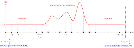
Figure 1.
Example 2-D problem geometry. In a periodic vacuum box, there is an arbitrarily-shaped inhomogeneous dielectric object. To extract traveling-wave normal modes of the system, we use Bloch-periodic boundary condition instead of periodic boundary condition under which only standing-wave normal modes can exist [36].
Using a countably-finite set ( number) of numerical normal modes, one can quantize a vector potential operator [36] as
where , , and are Bloch wavenumber, eigenfrequency, and mode-annihilation operator for m-th numerical normal mode, denoted by , respectively. The corresponding electric field operator becomes (based on gauge or generalized radiation or transverse gauge [38])
For convenience, we employ the linear algebra notation to represent the positive frequency component of (2) as
where , , , and Note that, in what follows, a boldface letter stands for a column vector and a boldface letter with a bar represents a matrix and a dimensionless quantity is measured in the unit of [one]. The numerical normal modes satisfy the orthonormal condition [2,39] as
where is the identity matrix, is a mass matrix, incorporating medium and metric properties, and is the Cholesky decomposition of , that is, ; hence, becomes a unitary matrix. It should be mentioned that both and are diagonal matrices when using a finite-difference method and their elements are given by and where . Consequently, the Hamiltonian operator can be diagonalized as
where and denotes the zero-point energy. One can think of numerical normal modes as uncoupled harmonic oscillators. Therefore, there is no energy coupling between different uncoupled harmonic oscillators; consequently, the Hamiltonian operator in the mode space becomes diagonalizable.
3. Quantization of Electromagnetic Fields in the Coordinate Space
3.1. Relation between Mode- and Coordinate-Ladder Operators
One can define coordinate-ladder (CL) operators, denoted by or , from mode-ladder (ML) operators via the unitary transformation or matrix shown in (4) as
where for n-th grid point. Inversely, one can also write
Note that CL operators still hold the commutator relation as
and the lowering and raising process as
Note that, in what follows, the index n is reserved to indicate n-th grid point (i.e., ) for CL operators.
3.2. Hamiltonian Operator in the Coordinate Space
By substituting (8) and (9) into (5), one finds that the Hamiltonian operator in the coordinate space becomes non-diagonalizable as
where is called hopping terms taking the form of
The hopping terms basically dictate the extent of energy coupling between different coupled harmonic oscillators. Unlike to the nearest hopping terms often used to model electron tunneling, Ising model, or coupled-resonator optical waveguides [32,33,40,41], the present hopping terms have the relatively long-range characteristics. These long-range hopping terms of the Hamiltonian operator play a key role in having the equivalence of solutions from Schrödinger-like quantum state equations (parabolic) and quantum Maxwell’s equations (hyperbolic). In other words, over-truncation of hopping terms for arbitrary EM environments may cause the significant amount of artificial dispersion errors to the quantum information propagation.
3.3. Electric Field Operator in the Coordinate Space
The new basis, denoted by , can be thought as a propagator for n-th CL operator (QEM-CV-propagator). For more intuitive understanding, consider n-th QEM-CV-propagator for the vacuum which can be simplified as
for . Except for the existence of , QEM-CV-propagators look quite similar to the classical counterpart (CEM-CV-propagator) [27,28] of which continuum expression can be defined by
In other words, the resultant classical (real-valued) fields are given by the sum of two convolutions which are equivalent to (1) the delta function sifting property and (2) the Hilbert transform w.r.t. as
where denotes the 1-D problem domain and is a complex-valued intial field scalar value at . Note that the Hilbert transform plays a key role to model one-way wave propagations, provided that a set of describes the phasor form of one-way traveling waves. This formulation is particularly feasible to deal with a wave equation (for a single-species unknown variable) rather than Maxwell’s curl equations. It should be noted that previous classical 1-D Maxwell-curl-propagators [27,28,42] consist of the time-derivative of retard and advanced time-domain Green’s functions and are supposed to carry real-valued initial electric and magnetic field values as
where and are real-valued initial electric and magnetic field values at and is a unit time-step function. As seen in (22), the underlying principle of one-way wave propagations is to cancel one of the two delta functions by controlling the initial electric or magnetic field values. In the quantum realm, positive- and negative-frequency components of QEM-CV-propagators become bases of annihilation and creation operators of which actions on quantum states have their own physical meaning such as annihilation and creation of photons, respectively. Thus, one has to treat positive- and negative-frequency propagators individually for quantum electromagnetics. The discrete representation of (20) can be written as
for .
One can think of QEM-CV-propagators as the convolution between the inverse Fourier transform of (band-limited) and CEM-CV-propagators (see Figure 2). Furthermore, employing the concept of fractional derivatives, one can associate CEM-CV-propagator with QEM-CV-propagator as
where denotes the half derivative w.r.t. time. As implied in (24), the vector space of the expectation value of the energy in the quantum regime becomes the subset of that of the classical EM energy. This results from the restriction to field amplitudes of quantum EM fields so as to enforce the energy of N number of photons in a monochromatic wave to be whereas there is no restriction in classical field amplitudes, hence, classical EM energy can take any positive real value. Figure 2 depicts an example of the temporal behaviors of a CEM-/QEM-CV-propagators. It is worth noting that the factor in (23) prevents to arrive at the correspondence principle between classical and quantum propagators even for the vacuum, that is, (23) and (20). This is a consequence of non-covariant normalization of the plane wave basis [43]. The invariant normalization approach [43,44] can be used to eliminate the factor. We will investigate the invariant normalization approach for our future work.
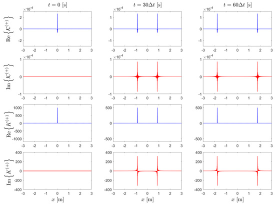
Figure 2.
Example of the temporal behaviors of quantum electromagnetic (complex-valued) (QEM-CV)-propagator and computational electromagnetic (complex-valued) (CEM-CV)-propagator when .
It should be emphasized that the concept of propagators for classical EM fields has been already discussed in References [27,28]. Their propagators are designed to carry real-valued initial field (scalar) values. However, propagators shown here can carry arbitrary complex-valued initial fields. Thus, it is suited to analyze the quantum nature of EM fields wherein probability amplitudes of quantum state can be arbitrary complex values as long as the normalization condition is satisfied.
Then, let us initialize a single photon spatially-localized at whose initial quantum state is given by . The expectation value of the electric energy operator, denoted by , for the single photon can be evaluated as
which corresponds to the half of the average value of all possible eigenenergies of the systems. Hence, we can say that QEM-CV-propagators describe how EM field operators are time evolving when a single photon is initialized at a certain grid, having its energy expectation value as . In other words, a single photon described in the coordinate space becomes more (and less) deterministic w.r.t. position (and energy). Note that the opposite situation happens in the mode space.
4. Quantum Finite-Difference Time-Domain Scheme
We have seen in the previous section that electric field operators could be expanded by CL operators weighted by QEM-CV-propagators which are given by the summation of numerical normal modes. However, there are no closed form solutions for general QEM-CV-propagators due to the energy scaling factor, viz., . Hence, we develop a quantum finite-difference time-domain scheme to numerically time evolve QEM-CV-propagators.
Here, we discretize the continuum of (16) and (23), that is, is the variable to be discretized in the present Q-FDTD scheme whereas denotes the position of initializing -th QEM-CV propagator. In other words, one can think of and . The Hamilton’s equations of motion (or wave equations) for the positive frequency component of electric field operators can be written as
Since coordinate-annihilation operators do not rely on space and time, the equation (27) can be further simplified by
It is to be noted that there should be no coupling between different QEM-CV-propagators; hence, one can independently find the time evolution of QEM-CV-propagators as
for . Applying a finite difference method to (29) w.r.t. space and time, one can derive the discrete counterpart of (29), called a quantum finite-difference time-domain (Q-FDTD) scheme, for n-th QEM-CV-propagator as
for where superscript l denotes time step and
Note that the above Q-FDTD scheme is embarrassingly-parallel due to the independence of index n while marching-on in time. Finally, numerical solutions of the electric field operator can be found as
5. Initial Quantum States for Few Photons
In the mode space, an initial quantum state for a single photon spatially localized in the form of Gaussian wavepacket is given by
where is a probability amplitude for , which corresponds to a spectral amplitude of the Gaussian wavepacket. Substituting (9) into (33), one can rewrite the initial quantum state in the coordinate space as
where and , , and are localization center position, localization degree, and carrier wavenumber of the Gaussian wavepacket, respectively, while satisfying the normalization condition . Note that one can also model wavepackets using Lorentzian or sinc functions.
An initial composite quantum state for non-entangled two (indistinguishable) photons can be given by the tensor product of each photon’s quantum state as
It is to be noted that (35) is invariant under the swapping process, viz., , since photons are assumed to be indistinguishable.
6. Initial Conditions of Quantum Finite-Difference Time-Domain Scheme
To run the Q-FDTD scheme, one needs initial values of QEM-CV-propagators and their time derivatives. Again, due to the non-existence of the closed form solutions for general QEM-CV-propagators, in order to get the initial values, one has to know numerical normal modes by solving the Helmholtz wave equations before running the Q-FDTD scheme, but, this becomes redundant.
Here, we show an alternative way of the initialization of the Q-FDTD scheme devoid of solving for the normal modes. First, assume that an initialized photon is spatially localized around in the vacuum. This allows one to only take into account some of QEM-CV-propagators that significantly affect the quantum information propagation. For example, one can select QEM-CV-propagators defined over grid point index where . Second, assume that the photon initialized in the vacuum is spatially far away from dielectric objects. In other words, the photon cannot recognize the presence of dielectric objects before touching them. As a result, QEM-CV-propagators can be approximated by analytic plane wave solutions as
for . Thus, the Q-FDTD scheme can be initialized by letting
7. Numerical Simulations of Quantum Beam Splitter
The Hong-Ou-Mandel effect [29] refers to a two-photon destructive interference effect in a 50/50 quantum beam splitter [45] and widely used in quantum optics experiments. Specifically, when a pair of photons is impinging on the beam splitter with the perfect temporal overlap, that is, , the two photons will always exit through a same output port while being bunched, having 50:50 chance of exiting from either one or the other output port. This is often measured through the degree of intensity coherence, called second order correlation, denoted as , originally related to the Hanbury Brown and Twiss (HBT) effect [46]. The quantum version of the second order correlation [47] is defined by
In our computer simulation, we set and , as illustrated in Figure 3, and . We used same simulation parameters used in Reference [36]. Also, One can evaluate (40) in the same way explained in Reference [36], which is the crucial part of creating quantum effects.
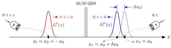
Figure 3.
Schematic of computer simulations for a quantum beam splitter to observe Hong-Ou- Mandel effect.
Figure 4 depicts versus for three different cases: (1) numerical canonical quantization, (2) Q-FDTD with exact initialization (with numerical normal modes obtained from solving the Helmholtz wave equation), and (3) Q-FDTD with approximate initialization by using from (36) to (39). There are excellent agreement in all cases, thus, the Q-FDTD scheme with approximate initialization is correctly validated. Furthermore, as expected, there are the HOM dips in all cases when since the destructive interference of the pair of photons occurs.
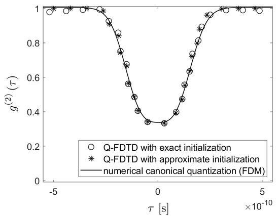
Figure 4.
The Hong-Ou-Mandel effects are numerically evaluated by using (1) numerical canonical quantization (solid line), (2) Quantum finite-difference time-domain (Q-FDTD) with exact initialization (round markers), and (3) Q-FDTD with approximate initialization (asterisk markers).
8. Conclusions
We have employed another approach to quantize electromagnetic (EM) fields in the coordinate space, instead of the mode space. In the coordinate space, EM field operators were expanded by coordinate-ladder operators weighted by non-orthogonal and spatially-localized bases, which were propagators of quantum electromagnetic initial field operators (QEM-CV-propagator). Due to the property of QEM-CV-propagators, the present formulation is suited to describe local features of photons. Since there were no closed form solutions available for them in arbitrary EM environments, we developed a quantum finite-difference time-domain method to numerically time evolve QEM-CV-propagators. In order to check the validity of the proposed quantum finite-difference time-domain scheme, we performed computer simulations to observe the two-photon indistinguishability in quantum beam splitters, known as the Hong-Ou-Mandel effect.
Author Contributions
Conceptualisation, D.-Y.N. and W.C.C.; Formal analysis, D.-Y.N. and W.C.C.; Funding acquisition, W.C.C.; Investigation D.-Y.N. and W.C.C.; Methodology, D.-Y.N. and W.C.C.; Project Administration, W.C.C.; Supervision, W.C.C. All authors have read and agreed to the published version of the manuscrip. All authors have read and agreed to the published version of the manuscript.
Funding
This research was funded by the National Science Foundation 1818910 award and a start up fund at Purdue University. W.C.C. was supported by DVSS Hong Kong University during the summer of 2019.
Acknowledgments
The work is funded by NSF 1818910 award and a startup fund at Purdue university.
Conflicts of Interest
The authors declare no conflict of interest.
References
- Chew, W.C.; Liu, A.Y.; Salazar-Lazaro, C.; Sha, W.E.I. Quantum electromagnetics: A new look-Part I. IEEE J. Multiscale Multiphys. Comput. Tech. 2016, 1, 73–84. [Google Scholar] [CrossRef]
- Chew, W.C.; Liu, A.Y.; Salazar-Lazaro, C.; Sha, W.E.I. Quantum electromagnetics: A new look-Part II. IEEE J. Multiscale Multiphys. Comput. Tech. 2016, 1, 85–97. [Google Scholar] [CrossRef]
- Cohen-Tannoudji, C.; Dupont-Roc, J.; Grynberg, G. Atom-Photon Interactions: Basic Processes and Applications; Wiley-VCH: New York, NY, USA, 1988. [Google Scholar]
- Mandel, L.; Wolf, E. Optical Coherence and Quantum Optics; Cambridge University Press: Cambridge, UK, 1995. [Google Scholar]
- Scheel, S.; Buhmann, S.Y. Macroscopic Quantum Electrodynamics. Acta Phys. Slov. 2008, 58, 675–809. [Google Scholar]
- Dirac, P.A.M.; Bohr, N.H.D. The quantum theory of the emission and absorption of radiation. Proc. R. Soc. Lond. Ser. A Contain. Pap. Math. Phys. Character 1927, 114, 243–265. [Google Scholar]
- Scully, M.O.; Zubairy, M.S. Quantum Optics; American Association of Physics Teachers (AAPT): College Park, MD, USA, 1999. [Google Scholar]
- Loudon, R. The Quantum Theory of Light; OUP Oxford: Oxford, UK, 2000. [Google Scholar]
- Gerry, C.; Knight, P. Introductory Quantum Optics; Cambridge University Press: Cambridge, UK, 2004. [Google Scholar]
- Vogel, W.; Welsch, D.G. Quantum Optics; John Wiley & Sons: Hoboken, NJ, USA, 2006. [Google Scholar]
- Walls, D.F.; Milburn, G.J. Quantum Optics; Springer Science & Business Media: Berlin, Germany, 2007. [Google Scholar]
- Garrison, J.; Chiao, R. Quantum Optics; Oxford University Press: Oxford, UK, 2008. [Google Scholar]
- Grynberg, G.; Aspect, A.; Fabre, C.; Cohen-Tannoudji, C. Introduction to Quantum Optics: From the Semi-Classical Approach to Quantized Light; Cambridge University Press: Cambridge, UK, 2010. [Google Scholar]
- Chew, W.C. Quantum Mechanics Made Simple: Lecture Notes; CreateSpace Independent Publishing Platform: Scotts Valley, CA, USA, 2015. [Google Scholar]
- Milonni, P. An Introduction to Quantum Optics and Quantum Fluctuations; Oxford Graduate Texts; Oxford University Press: Oxford, UK, 2019. [Google Scholar]
- Jauch, J.M.; Watson, K.M. Phenomenological Quantum-Electrodynamics. Phys. Rev. 1948, 74, 950–957. [Google Scholar] [CrossRef]
- Glauber, R.J.; Lewenstein, M. Quantum optics of dielectric media. Phys. Rev. A 1991, 43, 467–491. [Google Scholar] [CrossRef]
- Knöll, L.; Vogel, W.; Welsch, D.G. Action of passive, lossless optical systems in quantum optics. Phys. Rev. A 1987, 36, 3803–3818. [Google Scholar] [CrossRef]
- Huttner, B.; Barnett, S.M. Quantization of the electromagnetic field in dielectrics. Phys. Rev. A 1992, 46, 4306–4322. [Google Scholar] [CrossRef]
- Gruner, T.; Welsch, D.G. Green-function approach to the radiation-field quantization for homogeneous and inhomogeneous Kramers-Kronig dielectrics. Phys. Rev. A 1996, 53, 1818–1829. [Google Scholar] [CrossRef]
- Dalton, B.J.; Guerra, E.S.; Knight, P.L. Field quantization in dielectric media and the generalized multipolar Hamiltonian. Phys. Rev. A 1996, 54, 2292–2313. [Google Scholar] [CrossRef]
- Dung, H.T.; Knöll, L.; Welsch, D.G. Three-dimensional quantization of the electromagnetic field in dispersive and absorbing inhomogeneous dielectrics. Phys. Rev. A 1998, 57, 3931–3942. [Google Scholar] [CrossRef]
- Crenshaw, M.E. Comparison of quantum and classical local-field effects on two-level atoms in a dielectric. Phys. Rev. A 2008, 78, 053827. [Google Scholar] [CrossRef]
- Philbin, T.G. Canonical quantization of macroscopic electromagnetism. New J. Phys. 2010, 12, 123008. [Google Scholar] [CrossRef]
- Sha, W.E.I.; Liu, A.Y.; Chew, W.C. Dissipative Quantum Electromagnetics. J. Multiscale Multiphys. Comput. Tech. 2018, 3, 198–213. [Google Scholar] [CrossRef]
- Smith, B.J.; Raymer, M.G. Photon wave functions, wave-packet quantization of light, and coherence theory. New J. Phys. 2007, 9, 414. [Google Scholar] [CrossRef]
- Barton, G. Elements of Green’s Functions and Propagation: Potential, Diffusion, and Waves; Clarendon Press: Oxford, UK, 1989. [Google Scholar]
- Nevels, R.; Jeong, J. The time domain Green’s function and propagator for Maxwell’s equations. IEEE Trans. Antennas Propag. 2004, 52, 3012–3018. [Google Scholar] [CrossRef]
- Hong, C.K.; Ou, Z.Y.; Mandel, L. Measurement of subpicosecond time intervals between two photons by interference. Phys. Rev. Lett. 1987, 59, 2044–2046. [Google Scholar] [CrossRef]
- Santori, C.; Fattal, D.; Vuckovic, J.; Solomon, G.S.; Yamamoto, Y. Indistinguishable photons from a single-photon device. Nature 2002, 419, 594–597. [Google Scholar] [CrossRef]
- Beugnon, J.; Jones, M.P.A.; Dingjan, J.; Darquié, B.; Messin, G.; Browaeys, A.; Grangier, P. Quantum interference between two single photons emitted by independently trapped atoms. Nature 2006, 440, 779–782. [Google Scholar] [CrossRef]
- Zhou, L.; Gong, Z.R.; Liu, Y.X.; Sun, C.P.; Nori, F. Controllable Scattering of a Single Photon inside a One-Dimensional Resonator Waveguide. Phys. Rev. Lett. 2008, 101, 100501. [Google Scholar] [CrossRef] [PubMed]
- Longo, P.; Schmitteckert, P.; Busch, K. Dynamics of photon transport through quantum impurities in dispersion-engineered one-dimensional systems. J. Opt. A Pure Appl. Opt. 2009, 11, 114009. [Google Scholar] [CrossRef]
- Yee, K. Numerical solution of initial boundary value problems involving maxwell’s equations in isotropic media. IEEE Trans. Antennas Propag. 1966, 14, 302–307. [Google Scholar] [CrossRef]
- Taflove, A.; Hagness, S.C. Computational Electrodynamics: The Finite-Difference Time-Domain Method, 3rd ed.; Artech House: Norwood, MA, USA, 2005. [Google Scholar]
- Na, D.Y.; Zhu, J.; Teixeira, F.L.; Chew, W.C. Quantum Information Propagation Preserving Computational Electromagnetics. arXiv 2019, arXiv:1911.00947. [Google Scholar]
- Joannopoulos, J.D.; Johnson, S.G.; Winn, J.N.; Meade, R.D. Photonic Crystals: Molding the Flow of Light, 2nd ed.; Princeton University Press: Princeton, NJ, USA, 2008. [Google Scholar]
- Jackson, J.D. Classical Electrodynamics, 3rd ed.; Wiley: New York, NY, USA, 1999. [Google Scholar]
- Chew, W.C. Waves and Fields in Inhomogeneous Media; IEEE Press: Piscataway, NJ, USA, 1996. [Google Scholar]
- Miller, D.A. Quantum Mechanics for Scientists and Engineers; Cambridge University Press: Cambridge, UK, 2008. [Google Scholar]
- Kusminskiy, S.V. Quantum Magnetism, Spin Waves, and Light. arXiv 2018, arXiv:1807.10626. [Google Scholar]
- Shin, J. Time-Domain Propagator Full-Wave Numerical Method for Electromagnetic Fields. Ph.D. Thesis, Texas A&M University, Uvalde, TX, USA, 2018. [Google Scholar]
- Itzykson, C.; Zuber, J. Quantum Field Theory; International Series In Pure and Applied Physics; McGraw-Hill: New York, NY, USA, 1980. [Google Scholar]
- Hawton, M. Maxwell quantum mechanics. Phys. Rev. A 2019, 100, 012122. [Google Scholar] [CrossRef]
- Prasad, S.; Scully, M.O.; Martienssen, W. A quantum description of the beam splitter. Opt. Commun. 1987, 62, 139–145. [Google Scholar] [CrossRef]
- Hanbury-Brown, R.; Twiss, R. Interferometry of the intensity fluctuations in light—I. Basic theory: The correlation between photons in coherent beams of radiation. Proc. R. Soc. Lond. Ser. A Math. Phys. Sci. 1957, 242, 300–324. [Google Scholar]
- Glauber, R.J. The Quantum Theory of Optical Coherence. Phys. Rev. 1963, 130, 2529–2539. [Google Scholar] [CrossRef]
© 2020 by the authors. Licensee MDPI, Basel, Switzerland. This article is an open access article distributed under the terms and conditions of the Creative Commons Attribution (CC BY) license (http://creativecommons.org/licenses/by/4.0/).